www.ann-geophys.net/28/1795/2010/ doi:10.5194/angeo-28-1795-2010
© Author(s) 2010. CC Attribution 3.0 License.
Annales
Geophysicae
Interpolation of externally-caused magnetic fields over large sparse
arrays using Spherical Elementary Current Systems
S. A. McLay1and C. D. Beggan2
1School of GeoSciences, University of Edinburgh, West Mains Road, Edinburgh, EH9 3JW, UK 2British Geological Survey, Murchison House, West Mains Road, Edinburgh, EH9 3LA, UK
Received: 22 July 2010 – Revised: 25 August 2010 – Accepted: 15 September 2010 – Published: 30 September 2010
Abstract. A physically-based technique for interpolating
ex-ternal magnetic field disturbances across large spatial areas can be achieved with the Spherical Elementary Current Sys-tem (SECS) method using data from ground-based magnetic observatories. The SECS method represents complex elec-trical current systems as a simple set of equivalent currents placed at a specific height in the ionosphere. The magnetic field recorded at observatories can be used to invert for the electrical currents, which can subsequently be employed to interpolate or extrapolate the magnetic field across a large area. We show that, in addition to the ionospheric currents, inverting for induced subsurface current systems can result in strong improvements to the estimate of the interpolated magnetic field. We investigate the application of the SECS method at mid- to high geomagnetic latitudes using a series of observatory networks to test the performance of the exter-nal field interpolation over large distances. We demonstrate that relatively few observatories are required to produce an estimate that is better than either assuming no external field change or interpolation using latitudinal weighting of data from two other observatories.
Keywords. Geomagnetism and paleomagnetism (Rapid
time variations) – Ionosphere (Electric fields and currents; Modeling and forecasting)
1 Introduction
The geomagnetic field measured on the surface of the Earth is composed of temporally and spatially varying compo-nents. The primary sources include (1) the main field gen-erated in the outer core, (2) the crustal field and (3) fields produced by solar-terrestrial interaction. Electrical currents
Correspondence to: C. D. Beggan ([email protected])
induced in the subsurface are a secondary source contribu-tion to the measured magnetic field, but can be significant. Any surface measurement is a summation of these different fields at each instant of time. On time periods of seconds to days, changes in the magnetic field are principally of exter-nal origin and are caused by the solar wind, magnetosphere and ionosphere/upper atmosphere interaction (e.g. Campbell, 2003).
The study of temporal changes in the geomagnetic field and the accompanying induced electric fields are of inter-est in Earth hazard research. There are two classes of tech-nology that are adversely impacted by space weather: those directly affected by variations in the geomagnetic field and those affected by the electric currents induced by the chang-ing field. Modern applications of space weather studies to ground-based technology consider the problems of geomag-netically induced currents within power grids, oil and gas pipelines, telecommunication cables and railway equipment (Boteler et al., 1998; Pirjola et al., 2000; Pirjola, 2005). In-directly, geomagnetic disturbances in the ionosphere/upper atmosphere can disrupt the operation of technology exploit-ing real-time satellite data, such as positionexploit-ing and naviga-tion systems (e.g. Klobuchar, 1986). Estimates of external magnetic field values are often required at locations where it may not be possible or practical to make accurate measure-ments. For example, hydrocarbon exploration and produc-tion often demands real-time geomagnetic reference data at offshore oilfields around the UK and at other high latitude re-gions (Reay et al., 2005). Using real-time external field data aids accuracy in positional control of directional boreholes for safer extraction of oil and gas in challenging reservoirs (Bowe and McCulloch, 2007).
induced in the subsurface can also produce significant mag-netic field disturbances. During sub-storm onset their contri-bution can be up to 40% of the total observed change (Tan-skanen et al., 2001). The magnetic effects of telluric currents can also be modelled as equivalent currents. These can be constructed to lie within the subsurface and the superposi-tion of their magnetic effect with the ionospheric contribu-tion can be used to calculate the total ground magnetic field disturbance.
Several techniques have been developed to calculate equivalent currents from ground-based measurements; two of the most successful thus far have been the Fourier method (Mersmann et al., 1979) and Spherical Cap Harmonic Anal-ysis (SCHA) (Haines, 1985). The Fourier method assumes planarity of the Earth’s surface which limits its spatial ap-plicability, while the SCHA method employs global wave-length cut-offs and consequently is prone to aliasing effects, particularly with noisy data. A third approach, the Spheri-cal Elementary Current System (SECS) method, was estab-lished and developed by Amm (1997) and Amm and Vilja-nen (1999) respectively. The use of SECS overcomes some of the limitations of the other two methods and is suitable for studies both on a local and global scale. Amm and Vilja-nen (1999) demonstrated that the SECS technique produced a better fit than SCHA to simulated ionosphere conditions, while Pulkkinen et al. (2003b) showed it to be applicable for the interpolation of ionospheric fields in a densely sampled, relatively small region of northern Scandinavia.
In this paper we use the SECS method to interpolate exter-nal magnetic field disturbances over large spatial areas using relatively few input observatories. We test the method with data from networks of magnetometers in North America, around the North Sea and in Central Europe. The ability to model large and complex current variations in the ionosphere is investigated, as well as the adaptability to different spatial network configurations and scales. In Sect. 2 we briefly cover the theory of SECS and the computational framework for the interpolation of magnetic field disturbances. In Sect. 3 we describe the data used in the study and in Sect. 4 we illus-trate the resulting interpolation from the SECS method by comparison to measured observatory data. We discuss the applications and limitations of the technique in Sect. 5.
2 Spherical Elementary Current Systems
Ionospheric currents form a complex 3-D system, compris-ing three distinct current flows: Hall, Pedersen and field-aligned currents (FACs) (Ritter et al., 2004). By assum-ing sets of uniform conductance within the ionosphere and by using Ampere’s law, Fukushima (1976) first showed that magnetic perturbations produced by Pederson currents and FACs cancel each other below the base of the ionosphere. As the curl-free part of the current system Jcf is associated
with FACs it will produce no magnetic effect below the
de-fined base of the ionosphere. (Note, this property is actu-ally valid independently of how the currents are produced, i.e. it does not depend on the type of current flowing in the ionosphere or whether the conductances are uniform or not.) The curl-free system and therefore measurements at the sur-face of the Earth can neglect these effects. As a result of this simplification, ground magnetic field disturbances can be ob-tained from an exclusively divergence-free system of equiva-lent currents at a specific height in the ionosphere. A similar approach can be taken in the subsurface, by placing the ele-mentary current systems at an appropriate depth. It is impor-tant to remember that ionospheric equivalent currents are not a true representation of the 3-D current systems in the iono-sphere or in the subsurface, but are 2-D current sheets that produce a similar magnetic effect.
2.1 Background
The basic concept of SECS is to construct the equivalent cur-rent system using a linear superposition of divergence-free elementary current systems, all of which can be placed freely within the current plane. Amm (1997) defined a divergence-free system of spherical elementary sheet currents, Jdf,
us-ing a spherical coordinate system(r,θ,φ)with unit vectors (er,eθ,eφ)such that the poles of the elementary systems are
at their centres. With this description current sheets can be defined for the ionosphere and the subsurface:
Jextdf (r,θ )= I e
4π RS
cot
θ
2
eφ (1)
Jintdf(r,θ )= I i
4π RG
cot
θ
2
eφ (2)
In this descriptionIeandIiare the scaling factors for both external and internal divergence-free current systems andRS
andRGare the radius of the ionosphere and the depth of
in-ductance in the ground, respectively. These radii are defined in this study as infinitely thin layers 110 km above the Earth’s surface and 100 km beneath the Earth’s surface. By apply-ing Helmholtz’s theorem to Eqs. (1) and (2), Amm (1997) demonstrated that any ionospheric current distribution may be constructed uniquely by placing the poles of elementary systems within a plane.
The method developed in Amm and Viljanen (1999) in-troduced the continuation of the magnetic field disturbance from the ground to the ionosphere using SECS placement. Pulkkinen et al. (2003a) extended the complex image method of Pirjola and Viljanen (1998) to show that the field could be calculated from superposition of the magnetic effect of two horizontal current layers composed of divergence-free ele-mentary current systems. Their derivation is constructed for a point at radiusrbetween the current system in the ground and in the ionosphere,RG< r < RS for a position (θ,φ) on
effect of these two layers of horizontal currents consisting of a series of elementary current systems:
B(r,θ,φ)= L X
j=1
IjiTdfi(RG,θj,φj,r,θ,φ) (3)
+ M X k=1
IkeTdfe(RS,θk,φk,r,θ,φ)
whereTdfe andTdfi are the geometric parts of the external and internal magnetic fields produced by each elementary cur-rent system located at(RG,θj,φj)and(RS,θk,φk). L and
M, with subscripts j andk, denote the number of current systems solved for within the ground and at the radius of the ionosphere, respectively. Formulation of the magnetic field superposition is given in Appendix A of Pulkkinen et al. (2003a).
2.2 Inversion for current system scalings
We assume that the magnetic field vectorBhas been mea-sured at a set of points and construct a linear system of equa-tions relating the measured field to the geometric parts and scaling factors of both the internal and external elementary current systems. Expressing this in matrix form gives:
B=T·I (4)
We look to solve the linear inverse problem to determine the scaling factorsI of the internal and external elementary cur-rent systems. Due to the (generally) limited number of fixed ground magnetic observatories, the number of observation points is usually much lower than the number of elementary current systems required to produce a good representation of the actual currents. The linear inverse problem is therefore highly underdetermined:
I=T−1·B (5)
The matrix T may be badly conditioned which produces nu-merical instabilities when attempting to invert Eq. (5) di-rectly. Thus, we employ Singular Value Decomposition (SVD) for the inversion, truncating such that any eigenval-ues with an absolute value less than 1/100th of the largest are excluded from the solution, as suggested in Pulkkinen et al. (2003b). The truncation stabilises the inversion and tends to produce a slight smoothing effect on the solution. Other trun-cation levels were tested, including the truntrun-cation of eigen-values with an absolute value less than 1/10th of the largest value and also no truncation. The results were stable and in-deed quite similar; suggesting in these experiments that the
T matrix is not actually badly conditioned.
We solve for the scaling factors of the currents systems on a rectangular grid evenly-spaced in latitude and longitude (note, any reasonable shape and spacing could be used). The forward solution for the magnetic field (B) on the Earth’s surface at any position within the grid can be calculated by
determining the T matrix for the point of interest and using the scaling factors from the inversion.
Modelling was undertaken using minute mean magnetic field vector values. To prepare the data for inversion, the internal and crustal fields for each day were removed by sub-tracting the mean daily baseline values from the X, Y and Z components, giving a 24-h set of magnetic disturbance val-ues about the average. This deviation from the mean was used as the input into the B matrix and the positions of the observatories were used to construct the T matrix. The scal-ing factors (I) for the current systems across the grid of points were solved for every minute of the day.
The accuracy of the interpolation method is quantified by comparing the estimated magnetic field to data measured at an observatory which has not been used in the inversion. The root-mean-square (RMS) error (or misfit) between the esti-mated magnetic field and the measured field at timet can be calculated as:
RMS= v u u t
1 N
N X
t
Btobs−BtSECS2
(6)
where the subscript “obs” indicates the measured field at an observatory and “SECS” is the estimated field, for each of the three components of the magnetic field vector. The power of the measured data is described by the root-mean-square of the values, giving a coarse estimate of how magnetically disturbed the day was:
Power= v u u t
1 N
N X
t
BtObs2
. (7)
3 Investigation of controlling factors
We wish to investigate how well the SECS method can inter-polate the magnetic field across a region. It is assumed that the goodness of fit of the interpolation depends on several factors, including region size, the number of input observa-tories, and the relative spacing and location of the observato-ries. We also investigate the effect of relatively magnetically disturbed versus relatively quiet days, particularly in terms of the magnitude of the changes due to the external field and whether there are obvious differences e.g. due to the longi-tude offset of the observatories or perhaps induced currents.
2˚E 4˚E 6˚E
8˚E 10˚E 12˚E 14˚E 16˚E 18˚E 42˚N 44˚N 46˚N 48˚N 50˚N 52˚N 54˚N
0 100 200 km
Network 4 Network 5
160˚W
150˚W
140˚W
130˚W
120˚W
110˚W 100˚W 90˚W 80˚W
70˚W
60˚W 50˚W
40˚W
60˚N
60˚N
70˚N
70˚N
80˚N
80˚N
0 500 1000
km
Network 1 Network 2 Network 3
8˚W 6˚W
4˚W 2˚W 0˚ 2˚E 4˚E 6˚E 8˚E 10˚E
51˚N 52˚N
53˚N 54˚N
55˚N 56˚N
57˚N 58˚N
59˚N 60˚N
61˚N 62˚N
0 100 200 km
[image:4.595.69.530.63.545.2]Crooktree
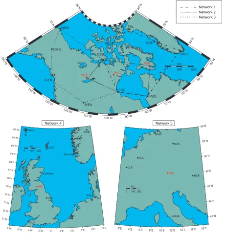
Fig. 1. Geographical arrangement of the five networks of magnetic observatories used in this study. The observatories used for comparison (denoted in red) for each network are: Network 1: IQA (Iqaluit); Network 2: BLC (Baker Lake); Network 3: YKC (Yellowknife); Net-work 4: ESK (Eskdalemuir); NetNet-work 5: FUR (Furstenfeldbruck). Observatories are denoted with the upper-case IAGA three-letter code. Variometers in Network 4 are denoted by their full name.
six observatories. Figure 1 shows the regions and observa-tories used in the study. Observaobserva-tories denoted in red are excluded from the inversion and are subsequently used to ex-amine how well the SECS method has estimated the field at their location. For each network, a rectangular grid of ele-mentary current systems evenly-spaced in latitude and longi-tude was constructed. In Networks 1–3, the grid spacing was
0 200 400 600 800 1000 1200 1400 -300
-200 -100 0 100 200
nT
0 200 400 600 800 1000 1200 1400
-300 -200 -100 0 100 200
nT
0 200 400 600 800 1000 1200 1400
-300 -200 -100 0 100 200
Minute
nT
Network 1: Iqaluit [IQA:63.75N; 291.48E]; Date: 11 Dec 2005
IQA X; Power = 69.4 SECS Estimate; Misfit = 51.6 Lat. Wgt. Estimate; Misfit = 55.3 SECS (Ext Only); Misfit = 54.2
IQA Y; Power = 62.8 SECS Estimate; Misfit = 40.2 Lat. Wgt. Estimate; Misfit = 67.6 SECS (Ext Only); Misfit = 44.4
[image:5.595.77.520.66.394.2]IQA Z; Power = 82.2 SECS Estimate; Misfit = 61.2 Lat. Wgt. Estimate; Misfit = 66.9 SECS (Ext Only); Misfit = 125.1
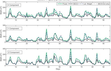
Fig. 2. Comparison of the measured external field disturbance (green solid, dots) and the estimate from SECS (black solid), Latitudinal Weighted (blue dashed) and SECS (External only) (grey dot-dash) at magnetic observatory Iqaluit (IQA) during a magnetically disturbed day (11 December 2005). Power and RMS misfit are in nT. Y-axis scaled to show finer details.
The magnetic field data were sourced from the World Data Centre for Geomagnetism (Edinburgh) and the Inter-national Real-time Magnetic Observatory Network (INTER-MAGNET) (Kerridge, 2001). The variometer data used in Network 4 were acquired from the UK Sub-Auroral Magne-tometer Network (SAMNET) data repository.
In addition, we tested two alternative implementations of the SECS equation. We solved solely for the external current elementary system scale value (Ie), thus excluding the inter-nal current systems (Ii). The external-only SECS (second term of Eq. 3) requires a solution for only half the number of parameters, and produces a different set of scaling factors compared to the solution using both the external and inter-nal elementary current systems. We also solved for the X and Y components of the external field to test if the solution improved when the Z component was ignored.
A further interpolation method was also used as a compar-ison to the interpolation of the SECS method. We employed the latitudinal-weighted average of measurements from two observatories, one to the south and one to the north of the
test observatory. In some networks, the two other observa-tories were not sited at a similar longitude to the test obser-vatory, leading to interpolation errors due to differences in local time, for example. Hence, the resulting error in the in-terpolation is strongly dependent on the relative positions of the two observatories, in both latitude and longitude.
4 Results
0 200 400 600 800 1000 1200 1400 -300
-200 -100 0 100 200
nT
0 200 400 600 800 1000 1200 1400
-300 -200 -100 0 100 200
nT
0 200 400 600 800 1000 1200 1400
-300 -200 -100 0 100 200
Minute
nT
Network 4: Eskdalemuir [ESK:55.32N; 3.2W]; Date: 11 Sep 2005
ESK X; Power = 56.1 SECS Estimate; Misfit = 13.7 Lat. Wgt. Estimate; Misfit = 34.8 SECS (Ext Only); Misfit = 25.9
ESK Y; Power = 34.4 SECS estimate; Misfit = 6.7 Lat. wgt. Estimate; Misfit = 10.1 SECS (Ext Only); Misfit = 26.3
[image:6.595.77.520.66.393.2]ESK Z; Power = 68.2 SECS Estimate; Misfit = 7.7 Lat. Wgt. Estimate; Misfit = 24.8 SECS (Ext Only); Misfit = 73.6
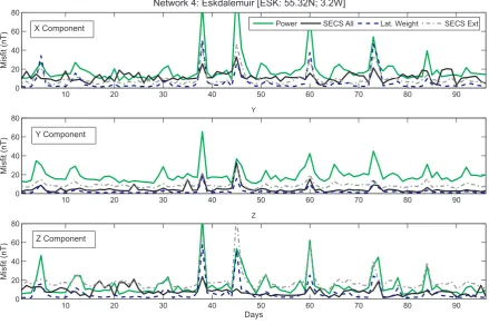
Fig. 3. Comparison of the measured external field disturbance (green solid, dots) and the estimate from SECS (black solid), Latitudi-nal Weighted (blue dashed) and SECS (ExterLatitudi-nal only) (grey dot-dash) at magnetic observatory Eskdalemuir (ESK) during a magnetically disturbed day (11 September 2005). Power and RMS misfit are in nT. Y-axis scaled to show finer details.
4.1 Magnetically disturbed vs. quiet day
For Networks 1–3, a magnetically disturbed day (11 Decem-ber 2005) with Kp of up to 5- and a magnetically quiet day (7 December 2005) with a Kp of 0 were chosen. Due to the availability of data for Networks 4 and 5, different days were selected: a magnetically disturbed day (11 September 2005) with Kp of up to 7- and a magnetically quiet day (21 Septem-ber 2005) with a Kp of 1+were used instead. The results on the magnetically disturbed days for Network 1 and Network 4 are given in Figs. 2 and 3.
Figure 2 shows the comparison of the measured data at the Iqaluit (IQA) observatory (green solid, dots) and the es-timate of the magnetic field from the SECS method using internal and external current systems (black solid) for Net-work 1. The estimate from interpolation using latitudinal weighting (blue dashed) of data from Qeqertarsuaq (GDH) and Narsarsuaq (NAQ) are also shown. Note both of these observatories are approximately 1000 km east of IQA. The SECS (External only) estimate solving only for an external set of current systems (grey dot-dash) is also plotted. The
es-timate from inverting the SECS equation with only the X and Y components was almost identical to the result for the SECS method using internal and external current systems and so is not plotted to avoid cluttering the figures.
10 20 30 40 50 60 70 80 90 0
100 200 300
Misfit (nT)
Network 1: Iqaluit [IQA:63.75N; 291.482E]
10 20 30 40 50 60 70 80 90
0 100 200 300
Misfit (nT)
10 20 30 40 50 60 70 80 90
0 100 200 300
Misfit (nT)
Days
Power SECS Lat. Weight SECS Ext only
Y Component
[image:7.595.78.520.69.354.2]Z Component X Component
Fig. 4. Comparison of the daily power of measured external disturbances (green solid) with the misfit estimate from the SECS (black solid), Latitudinal Weighted (blue dashed) and SECS (External only) (grey dot-dash) method over a three-month period (April-June 2005) at magnetic observatory Iqaluit (IQA).
Numerical estimates of the fit are given in figure legends (and also Table 1). For example, the power of the data (Eq. 7) in the Y component is 62.8 nT, while the RMS misfit of the SECS and the SECS (X and Y only) estimate is 40.2 nT and the SECS (External only) estimate is 44.4 nT. The misfit of the latitudinal weighted estimate is 67.6 nT, indicating that the variance of the latitudinal weighted estimate is worse than that of the data. If one had assumed no change occurred in the field due to the external field throughout the day for this component, it would have been (slightly) better than using the latitudinal weighted estimate. Thus, in the Y component the SECS method shows a strong improvement on the latitu-dinal weighting method, though the advantage gained from the SECS method is not as great in the X and Z components. In Network 4 (North Sea region), external field varia-tions recorded at Eskdalemuir (ESK) observatory during the magnetically active day exceeded 150 nT. Network 4 con-tains four observatories and four variometers, two of which (Crooktree and York) are relatively close to Eskdalemuir. The latitudinal weighted estimate uses data from Lerwick (LER) and Hartland (HAR) observatories.
Figure 3 compares the estimated magnetic field from the SECS and latitudinal weighted methods. The SECS estimate most closely matches the measured data, especially in the X
and Z components of the magnetic field where the largest variations are observed. In this case, the SECS method slightly underestimates the largest spikes seen in the mag-netic field disturbance (e.g. between minutes 75 and 400 in the X component), but is otherwise a good fit. The latitu-dinal weighted estimate overestimates the magnitude of the changes in the field, while the SECS (External only) estimate again compares well in X and Y but is extremely poor in Z. Note, the SECS (X and Y only) estimate is very similar to the SECS estimate and is not shown.
The misfits of the SECS estimate are consistently smaller than the power of the data and provide a significant improve-ment over the latitudinal weighted estimate for this day. The SECS (External only) estimate indicates that modelling of the ionospheric current sheets alone cannot account for the observed magnetic field changes in the Z component.
10 20 30 40 50 60 70 80 90 0
20 40 60 80
Network 4: Eskdalemuir [ESK: 55.32N; 3.2W]
Misfit (nT)
10 20 30 40 50 60 70 80 90
0 20 40 60 80
Y
Misfit (nT)
10 20 30 40 50 60 70 80 90
0 20 40 60 80
Z
Misfit (nT)
Days
Power SECS All Lat. Weight SECS Ext
X Component
Y Component
[image:8.595.79.519.65.356.2]Z Component
Fig. 5. Comparison of the daily power of measured external disturbances (green solid) with the misfit estimate from the SECS (black solid), Latitudinal Weighted (blue dashed) and SECS (External only) (grey dot-dash) method over a three-month period (April–June 2005) at magnetic observatory Eskdalemuir (ESK).
quiet days, the results of the latitudinal weighted method are comparable to the SECS method.
Scrutinising the results from Table 1 suggests that includ-ing a greater number of observatories (e.g. Network 1) low-ers the misfit, even if these are uncalibrated variometlow-ers (as in Network 4). At lower geomagnetic latitudes (Network 5) im-provements are not as marked. In Networks 2 and 3, which cover very large areas and have only five and seven obser-vatories, respectively, the SECS estimates are not as good, particularly in the Z component on disturbed days. For Net-works 1–4, the SECS (External only) estimate is extremely poor on disturbed days, again, particularly in the Z compo-nent suggesting that reasonable estimates of ground magnetic field disturbances require modelling of the induced magnetic field. By comparing the SECS (External only) mifits with the SECS (X and Y only) misfits, it is clear that solving for the X and Y components using the external field part of the SECS equation (i.e. ignoring the Z component) greatly im-proves the estimate. However, in general, the SECS (X and Y only solution) misfits are not consistently smaller than the misfits from solving for the internal and external parts of the field together.
4.2 Evaluation over three months
Approximately three months of observatory and variometer data from the beginning of April to start of July 2005 were analysed, comprising of several quiet and relatively disturbed periods. A comparison of the daily power of the data and the RMS misfit of the SECS estimate, the latitudinal weighted estimate and the SECS (External only) estimate for Net-work 1 are shown in Fig. 4. The SECS method provides a consistent improvement to the estimate compared to the lat-itudinal weighting estimate. Results for Networks 2 and 3 are similar. This longer time series analysis illustrates that the SECS method is most beneficial on disturbed days, but on quieter days the latitudinal weighting is actually a good proxy for the magnetic field, even at widely separated longi-tudes. The SECS (External only) estimate has, in general, a slightly larger misfit to the observed data in all components.
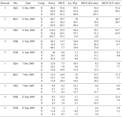
Table 1. RMS errors of the Power, SECS, Latitudinal Weighting, SECS (External only) and SECS (X and Y only) estimates for the five networks, calculated over a period of twenty-four hours. Analysis is presented for a magnetically disturbed day (11 December 2005; 11 September 2005) and magnetically quiet day (7 December 2005; 21 September 2005), depending on the availability of data within each network. For Network 1, the observatories used for latitude weighting are GDH and NAQ; Network 2 uses CBB and FCC; Network 3 uses CBB and MEA; Network 4 uses LER and HAD; Network 5 uses WNG and AQU.
Network Obs. Date Comp. Power SECS Lat. Wgt. SECS (Ext only) SECS (X;Y only)
1 IQA 11 Dec 2005 X 69.4 51.6 55.3 54.2 51.4
Y 62.8 40.2 67.6 44.4 40.2
Z 82.2 61.2 66.9 125.1 –
2 BLC 11 Dec 2005 X 69.7 59.7 78 52 60.7
Y 43.3 28.2 26.7 35.5 28.7
Z 81.9 65.1 68.4 123 –
3 YKC 11 Dec 2005 X 114.9 52.5 94.6 55.1 54.7
Y 52.6 65.1 57.7 51.3 63.5
Z 103.7 97.2 115 133 –
4 ESK 11 Sep 2005 X 56.2 13.7 34.8 25.9 13.4
Y 34.4 6.7 10.1 26.3 6.7
Z 68.2 7.7 24.8 73.6 –
5 FUR 11 Sep 2005 X 49 8.6 7.1 24.1 8.2
Y 24.1 4.8 5.2 11.1 4.8
Z 25.3 5.2 8.8 11.3 –
1 IQA 7 Dec 2005 X 12.6 7.5 10.5 8.2 7.6
Y 10.3 7.8 5.8 7.7 7.7
Z 12.8 10.5 11.6 12.3 –
2 BLC 7 Dec 2005 X 21.6 16.9 23 15.7 17.3
Y 15.3 9.2 10 10.4 7.7
Z 17.8 18.4 19.4 18.2 –
3 YKC 7 Dec 2005 X 8.9 6.3 12.1 6.8 6.5
Y 6.7 4.7 9.2 5 4.6
Z 7.7 8.3 13.7 21.7 –
4 ESK 21 Sep 2005 X 9.5 12.3 1.3 3.3 12.4
Y 9.3 1.6 0.6 4.3 1.6
Z 4.5 7.6 2.1 22.3 –
5 FUR 21 Sep 2005 X 7.4 2 1 4.2 1.9
Y 11.8 1.3 0.5 5.5 1.2
Z 4.3 0.7 1.5 3.6 –
is worse than assuming no external field change, which may be due to the inclusion of uncalibrated variometers, as the estimate misfit rarely falls below about 15 nT in the X and Z components. Interestingly, the SECS (External only) esti-mate has a lower average misfit in the X component, though is markedly poorer in Z.
5 Discussion
The external magnetic field and its influence on the ground magnetic field are still relatively poorly understood. The SECS method provides a flexible approach to modelling
has also been applied in the analysis of magnetospheric and ionospheric flow vortices with a large set of magnetome-ter stations in northern America, from Alaska to Green-land, involving a number of magnetometer arrays including THEMIS and CARISMA in combination with satellite-based observations (Keiling et al., 2009).
The improved estimate of the field from the SECS inter-polation method is very noticeable at high geomagnetic lat-itudes. The SECS estimate of the field is generally better than latitudinal weighting particularly during magnetically disturbed conditions. In magnetically quiet conditions the latitudinal weighting estimate is comparable or occasionally better. At lower geomagnetic latitudes, the SECS method again produces the lowest misfit during magnetically active conditions but performs less well in very quiet conditions. Modelling the magnetic field using only the external ele-mentary current systems produced misfits which were con-sistently poorer. This indicates that solving for internal cur-rent systems greatly improves the resulting estimate from the SECS method, particularly in the Z component.
Clearly, compared to latitudinal-based interpolation based on data from two observatories, there is a greater logisti-cal and computational cost in acquiring data from a larger number of observatories to use with the SECS method e.g. for real-time or practical purposes. However, if the data are available, the benefits from the improved estimate, particu-larly during noisy conditions, outweigh the slightly larger computational costs, as the inversion of the magnetic field data using Singular Value Decomposition and computation of the T matrix are extremely fast.
As a more sophisticated external field interpolation ap-proach, we suggest it could have applications in marine and aeromagnetic surveying, improving the ability to resolve the local crustal field, or perhaps in satellite magnetometry to re-move the effects of ionospheric currents for more accurate main field models. Other applications include better real-time estimates of the field for directional drilling and poten-tial prediction of geomagnetically-induced currents in power systems.
6 Conclusions
Interpolation of the magnetic field over large areas can be achieved using Spherical Elementary Current Systems. The method is derived from Maxwell’s equations and represents a physical rather than a mathematical approach to interpolation and extrapolation. We show that the method can be applied to produce good estimates of the magnetic field over large re-gions using data from a relatively small number of observa-tories. In addition to modelling external field variations, we found that including ground induced current systems gave a marked improvement in the estimate of the Z component of the magnetic field.
At high geomagnetic latitudes, the SECS method gave the best estimate of the external magnetic field, particularly dur-ing magnetically active days. At lower latitudes, durdur-ing mag-netically quiet periods, the SECS method is comparable to the latitudinal weighted average of two observatories, one approximately to the north and the other to the south of the point of interest.
We have shown that the SECS method can be applied to networks of different sizes where various densities of ob-servatory data are available. In situations where direct mea-surement of the external field is not possible due to logistical or physical constraints we suggest the SECS method can be used as a powerful interpolation tool.
Acknowledgements. We wish to acknowledge Allan McKay for de-velopment and initial coding of the algorithms used in this study. We thank O. Amm for his thorough review and suggestions for im-proving the manuscript. The institutes that support magnetic ob-servatories together with INTERMAGNET are thanked for promot-ing high standards of observatory practice. INTERMAGNET data was obtained from the World Data Centre (Edinburgh). The Sub-Auroral Magnetometer Network data (SAMNET) is operated by the Department of Communications Systems at Lancaster Univer-sity (UK) and is funded by the Science and Technology Facilities Council (STFC). This paper is published with the permission of the Executive Director of the British Geological Survey (NERC).
Topical Editor K. Kauristie thanks O. Amm for his help in eval-uating this paper.
References
Amm, O.: Ionospheric elementary current systems in spherical co-ordinates and their application, J. Geomag. Geoelectr., 49, 947– 955, 1997.
Amm, O. and Viljanen, A.: Ionospheric disturbance magnetic field continuation from the ground to the ionosphere using spherical elementary current systems, Earth Planets Space, 51, 431–440, 1999.
Boteler, D., Pirjola, R., and Nevanlinna, H.: The effects of geomag-netic disturbances on electrical systems at the Earth’s surface, Adv. Space Res., 22, 17–27, 1998.
Bowe, J. and McCulloch, S.: Space Weather, chap. The value of real-time geomagnetic reference data to the oil and gas industry, pp. 289–298, Springer, 2007.
Campbell, W.: Introduction to Geomagnetic Fields, Cambridge University Press., 2003.
Haines, G.: Spherical cap harmonic analysis, J. Geophys. Res., 90, 2583–2591, 1985.
Keiling, A., Angelopoulos, V. Runov, A., Weygand, J., Apatenkov, S. V., Mende, S., McFadden, J., Larson, D., Amm, O., Glass-meier, K.-H., and Auster, H. U.: Substorm current wedge driven by plasma flow vortices: THEMIS observations, J. Geophys. Res., 114, A00C22, doi:10.1029/2009JA014114, 2009. Kerridge, D.: INTERMAGNET: Worldwide near-real-time
Klobuchar, J.: Ionospheric time-delay algorithm for single-frequency GPS users, IEEE Transactions on Aerospace and Elec-tronics System, 23, 325–331, 1986.
Mersmann, U., Baumjohann, W., K¨uppers, F., and Lange, K.: Anal-ysis of an Eastward Electrojet by means of upward continuation of ground-based magnetometer data, J. Geophys., 45, 281–298, 1979.
Pirjola, R.: Effects of space weather on high-latitude ground sys-tems, Adv. Space Res., 36, 2231–2240, 2005.
Pirjola, R. and Viljanen, A.: Complex image method for cal-culating electric and magnetic fields produced by an auro-ral electrojet of finite length, Ann. Geophys., 16, 1434–1444, doi:10.1007/s00585-998-1434-6, 1998.
Pirjola, R., Viljanen, A., Pulkkinen, A., and Amm, O.: Space weather risk in power systems and pipelines, Phys. Chem. Earth, 25, 333 –337, 2000.
Pulkkinen, A., Amm, O., Viljanen, A., and BEAR Working Group: Separation of the geomagnetic field variation on the ground into external and internal parts using the spherical elementary current system method, Earth Planets Space, 55, 117–129, 2003a. Pulkkinen, A., Amm, O., Viljanen, A., and BEAR Working Group:
Ionospheric equivalent current distributions determined with the method of spherical elementary current systems, J. Geophys. Res., 108, 1053, doi:10.1029/2001JA005085, 2003b.
Reay, S. J., Allen, W., Baillie, O., Bowe, J., Clarke, E., Lesur, V., and Macmillan, S.: Space weather effects on drilling ac-curacy in the North Sea, Ann. Geophys., 23, 3081–3088, doi:10.5194/angeo-23-3081-2005, 2005.
Ritter, P., L¨uhr, H., Viljanen, A., Amm, O., Pulkkinen, A., and Sil-lanp¨a¨a, I.: Ionospheric currents estimated simultaneously from CHAMP satelliteand IMAGE ground-based magnetic field mea-surements: a statisticalstudy at auroral latitudes, Ann. Geophys., 22, 417–430, doi:10.5194/angeo-22-417-2004, 2004.
Tanskanen, E. I., Viljanen, A., Pulkkinen, L., Pirjola, R., H¨akkinen, L., Pulkkinen, A., and Amm, O.: At substorm onset, 40% of AL comes from underground, J. Geophys. Res., 106, 13119–13134, 2001.
Vanham¨aki, H., Amm, O., and Viljanen, A.: One-dimensional up-ward continuation of the ground magnetic field disturbance using spherical elementary current systems, Earth Planets Space, 55, 613–625, 2003.