Exchanges
Exchanges
CLIVAR is an international research programme dealing with climate variability and pre-dictability on time-scales from months to centuries.
October 2006 No 39 (Volume 11 No 4)
CLIVAR is a component of the World Climate Research Programme (WCRP). WCRP is sponsored by the World Meteorological Organization, the International Council for Science and the Intergovernmental Oceanographic Commission of UNESCO.
20°E 40°E 60°E 80°E 100°E 120°E
-40°S -30°S -20°S -10°S 0° 10°N 20°N 30°N
Repeat CTD/Carbon lines Frequently repeated XBT lines High resolution XBT and flux lines
Also included are the 3°x3° Argo profiling float array, 5°x5° surface drifting buoy array and a real-time and near real-time tide gauge network (20 stations in operation with ~20 planned)
Surface moorings Flux reference sites ADCP
Indian Ocean Climate
From Meyers and Boscolo, page 2: The Indian Ocean Observing System (IndOOS)
Editorial
As you will see, this edition of Exchanges focuses on Indian Ocean Climate. A key activity of the joint CLIVAR/IOC GOOS Indian Ocean Panel has been to develop a plan for sustained observations over the Indian Ocean region, summarized in the paper by Gary Meyers and Roberta Boscolo. As it works to encourage implementation of this plan through national agencies and international ocean observation coordination mechanisms, illustrated by the paper by Mike McPhaden et al., the panel is also seeking to develop the science of the Indian Ocean’s role in climate. It will do this in particular in conjunction with CLIVAR’s Asian-Australian Monsoon and Variability of the African Climate System Panels. Linking these activities to the wider role of the Pacific in the climate system and CLIVAR activities in seasonal to interannual, decadal and climate change prediction is also a key integrating role for CLIVAR overall. Papers here represent recent developments in Indian Ocean observational and modelling studies. In addition, this edition also carries reports of two CLIVAR-related workshops, one linking the International Climate of the 20th Century Project and CLIVAR efforts in seasonal to interannual prediction and the other on much longer timescales - the joint PAGES/CLIVAR Workshop on past-millennia climate variability, illustrating the breadth and range of CLIVAR. The next edition of Exchanges (January 2007) will be joint with the International Council for the Exploration of the Sea (ICES) and will focus on North Atlantic and Nordic Sea climate variability.
The circulation and transport of heat in the Indian Ocean is unique in many respects, compared to the Pacific and the Atlantic. The Asian landmass blocks the ocean in the north so that currents cannot carry tropical heat to higher latitude as the Atlantic and Pacific do. It also receives extra heat from the Pacific via the Indonesian Throughflow. The movement of heat around the ocean and exchange with the atmosphere is highly variable in time. As a consequence, the Indian Ocean plays a unique role in the variation of regional and global climate systems.
Indian Ocean climate research has been limited in the past by a very sparse historical record of oceanographic and marine meteorological observations. Never-the-less, the research-issues that have to be addressed have been identified. The key issues are:
• Seasonal monsoon variability, in particular the role of seasonal variation in oceanic circulation and heat transport
• Intraseasonal variability, in particular air-sea interaction, and what, if any, role does oceanic dynamics play in the longer time-scales of weather prediction
• Indian Ocean zonal dipole mode, El Nino–Southern Oscillation and their mutual interactions
• Decadal variation of all of the above, and warming trends in the upper Indian Ocean
• Southern Indian Ocean, one of the most sparsely sampled regions of the world, and its role in climate variability • The unique features of Indian Ocean circulation and their
role in the global heat budget, including the Indonesian Throughflow, the shallow subtropical-tropical overturning cell that affects sea surface temperature on both sides of the equator, and the inter-ocean exchange with the Atlantic • Biogeochemical cycling in the Indian Ocean.
The societal and economic impacts of these climate variations affect the lives of nearly hundreds of millions of the world’s population. The benefit to be derived from describing, understanding, modelling and predicting the coupled ocean– atmosphere behaviour in this region is potentially huge. The CLIVAR-GOOS Indian Ocean Panel (IOP) (http://www. clivar.org/organization/indian/indian.php) has prepared an implementation plan to collect essential data required to support research on these issues. The plan is available for download at: http://eprints.soton.ac.uk/20357/01/IOP_Impl_Plan.pdf. It provides a brief overview of each of the above research-issues, and technical details on a basin-scale, integrated observing system (Figure 1, front cover). Integration implies that we make use the technologies for in situ data collection that have proven to be sustainable and useful for climate research in the long term, as well as integration with the available satellite based measurements of sea surface temperature, sea level, wind and ocean colour. Plans for physical measurements are better developed at this stage than plans for biogeochemical measurements; however, integration across physics, chemistry and biology is also anticipated.
The technologies available for large-scale ocean monitoring are moorings (for subsurface temperature, salinity, currents, biogeochemical sensors and surface weather variables), Argo floats (for subsurface temperature, salinity and oxygen), expendable bathythermograph (XBT) lines, surface drifters (for
sea-surface temperature and current) and sea-level stations. The key new element of the observing system is a basin-scale mooring array (see McPhaden et al. this issue), which is essential to capture the seasonal monsoon variability and intraseasonal disturbances. As well as measurements of oceanic variables, the meteorological measurements at moorings provide much needed data to validate and calibrate estimates of surface fluxes from satellite data and they will be extremely valuable to data assimilation issues concerned with weather forecasting and reanalysis efforts.
The Argo Programme to measure temperature and salinity profiles to a depth of ~1500 m every 10 days is progressing rapidly in the Indian Ocean. The standard sampling pattern requires 450 floats to cover the ocean to 40°S with one float per 3°×3° latitude/longitude. Sustained monitoring will require 125 deployments per year, assuming a float lifetime of 3-4 years. As a minimum the standard Argo array in the Indian Ocean should be completed and maintained. The Argo profiles are essential for research on the role of ocean circulation in climate variability and change, from interannual to multidecadal time-scales. The XBT network in the Indian Ocean was initiated during TOGA and WOCE, but never fully implemented. XBT lines are effective for monitoring specific ocean structures that affect climate, such as the Indonesian Throughflow and upwelling zones between Java and Australia and the thermocline ridge near 10°S, both areas of documented strong ocean-atmosphere interaction. A trans-equatorial line in the western Indian Ocean can monitor inflow to the western boundary currents. The IOP critically reviewed the TOGA-WOCE XBT lines in preparing the plan, with regard to scientific justification, potential impact on future research and feasibility of implementation. The high-priority lines were determined to be IX01, IX08, IX09N/IX10E, IX12, IX22 and PX-02 for the so-called frequently repeated (FRX) sampling mode; and IX1, IX15/IX21 for the high-density (HDX) sampling mode. The value of other lines is discussed in the report as well.
The International Buoy Programme for the Indian Ocean (IBPIO) was formally established in 1996 and has become the primary body for coordinating multinational activities to implement surface drifting buoys. The drifter array was originally designed for reduction of the bias error in satellite SST measurements, and called for one drifter per 5° square. IOP noted that a re-evaluation of the sampling density is required for direct measurement of surface current, a growing need as ocean-reanalysis products require validation.
The international response to the Indian Ocean tsunami disaster in December 2004 is the rapid development of an Indian Ocean Tsunami Warning and Mitigation System (IOTWS). This development will potentially have numerous synergies with the development of IndOOS. In particular, the network of sea level stations is being upgraded to real-time monitoring at numerous locations. The IOTWS community is working closely with the climate-community to ensure that the upgraded sea level stations will also serve the purpose of climate research. Design of biogeochemical sampling is at an early stage compared to physical sampling. The implementation plan identifies initial ideas for Indian Ocean observations, including repeat hydrographic sections, recently developed sensors on The Indian Ocean Observing System (IndOOS)
Meyers G.1 and R. Boscolo2, . 1CSIRO Hobart Australia. 2ICPO Spain
ships of opportunity, and biogeochemical sensors on the basin-scale mooring array and Argo floats.
Clearly, full implementation of IndOOS will require a well-coordinated, international effort of large magnitude. One or just a few nations cannot carry the full investment of resources. The implementation plan includes a set of principles that is
meant to encourage broad international participation and rapid transition of measurements to societal benefit. Chief among the principles is the need to distributed data openly in a timely manner. There is a preference for communication of data in real time to make it available at climate analysis and prediction centers. This is essential to demonstrate the value of IndOOS and capture the potential societal benefits.
1. Introduction
The Indian Ocean is unique among the three tropical ocean basins in that it is blocked at 25°N by the Asian land mass. Seasonal heating over this land mass sets the stage for dramatic monsoon wind reversals and intense summer rains over the Indian subcontinent and adjoining areas of Southeast Asia. Recurrence of these summer monsoon rains is critical to agricultural production that provides life-sustaining support for hundreds of millions of people in the region. The reversing monsoon winds also generate a unique system of currents unlike those observed in the tropical Atlantic and Pacific, which are under the influence of steadier trade winds. Blocked by Asia, these currents cannot export heat to the northern subtropics. The resulting oceanic thermal structure produces feedbacks to the overlying atmosphere that affect not only the monsoon circulation and rainfall patterns, but also weather and climate in remote parts of the globe through atmospheric teleconnections.
Despite the importance of the Indian Ocean in the regional and global climate system, it is the most poorly observed and least well understood of the three tropical oceans. To remedy this situation, the Indian Ocean Panel, sponsored by the Climate Variability and Predictability Program (CLIVAR) and the Global Ocean Observing System (GOOS), has developed a plan for systematic, sustained, and comprehensive in situ observations in the Indian Ocean to complement both present and planned space-based satellite measurements. The plan (available at http://eprints.soton.ac.uk/20357/01/ IOP_Impl_Plan.pdf) describes the scientific rationale, design criteria and implementation strategies for each of the observing system components. These include Argo floats, drifting buoys, tide gauge stations, ship-of-opportunity expendable bathythermograph (XBT) lines, a basin scale moored buoy array, and specialized measurement programs for the Indonesian Throughflow and western boundary currents. India also maintains a regional national buoy program in the Bay of Bengal and Arabian Sea. The totality of these efforts is referred to as the Indian Ocean Observing System (IndOOS) (Meyers and Boscolo, this issue). This article focuses on specific issues related to design and implementation of the basin scale moored buoy array component of IndOOS.
2. Scientific Rationale and Design Goals
Mooring programs have been implemented in the Indian Ocean in the past as part of CLIVAR, the World Ocean Circulation Experiment (WOCE), the Joint Global Ocean Flux (JGOFS) experiment, and various national initiatives. In most cases though, these programs were relatively short term and/or focused on a particular region. Missing until recently was a plan for a coordinated, multi-national, basin-scale sustained mooring array like the Tropical Atmosphere Ocean/Triangle Trans-Ocean Buoy Network (TAO/TRITON) in the Pacific
Development of an Indian Ocean Moored Buoy Array for Climate Studies
McPhaden M.J.1, Y. Kuroda2 and V. S. N. Murty3,
1NOAA/Pacific Marine Environmental Laboratory, USA, 2Japan Marine-Earth Science and Technology Agency, Japan, 3National
Institute of Oceanography, Goa, India
Corresponding author: [email protected]
and the Pilot Research Moored Array in the Tropical Atlantic (PIRATA).
The CLIVAR/GOOS Indian Ocean Panel moored buoy array is designed to resolve the most energetic variations in the open ocean away from the western boundary. Like the Pacific TAO/TRITON array, it is intended to be marginally coherent in latitude and longitude for defining the evolution of large-scale intraseasonal-to-interannual wind, sea surface temperature (SST), upper-ocean temperature and salinity variations. It is essential for understanding the role of the ocean in variability related to the Madden-Julian Oscillation (MJO) and other high frequency phenomena, for understanding mixed-layer dynamics, and for understanding interactions between the ocean and atmosphere. The data will also support development of operational climate forecast models, weather and climate prediction, ocean-state estimation, reanalysis efforts, and satellite validation.
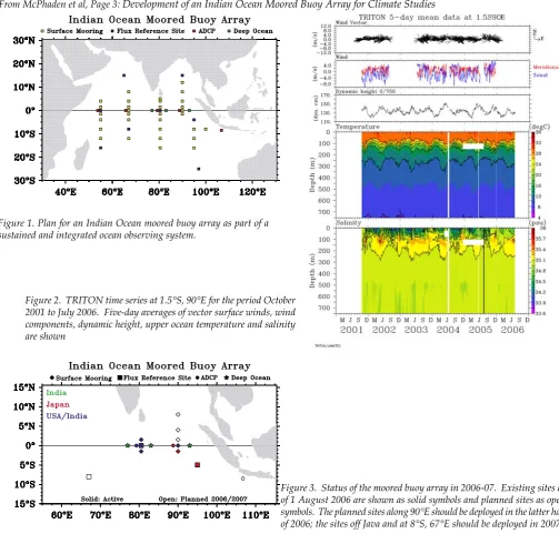
The array (Figure 1, page 15) consists of 39 surface moorings for measurement of temperature, salinity, mixed layer currents, and basic meteorological variables. Four subsurface Acoustic Doppler Current Profiler (ADCP) moorings are located along the equator where geostrophy breaks down and direct current measurements are necessary. A fifth ADCP mooring is also located in the upwelling zone off the Island of Java where the SST dipole/zonal mode first develops. This mooring is near the northern terminus of the frequently repeated XBT line IX1 between Australia and Indonesia. In addition to the 39 surface and 5 ADCP moorings, three subsurface moorings maintained by India’s National Institute of Oceanography (NIO) along the equator at 77°E, 83°E, and 93°E are designed to monitor deep ocean currents.
The entire array will contribute to the objectives of the OceanSITES program (http://www.oceansites.org/). In addition, eight specially enhanced flux reference sites will provide instrumentation to estimate all components of surface heat, moisture and momentum fluxes. These enhanced moorings are located in different climatic zones where climatologies are poorly known or where surface fluxes are critical for understanding climate variability (Yu et al, 2006). 3. Status of Implementation
The Japan Marine-Earth Science and Technology Agency (JAMSTEC) pioneered the deployment of long-term moorings for studies of ocean-atmosphere interactions in the Indian Ocean with an ADCP mooring at 0°, 90°E in 2000 (Masumoto et al, 2005) and two TRITON moorings at 1.5°S, 90°E and 5°S, 95°E in 2001 (Figure 2, page 15). Deep ocean subsurface moorings were also initiated by NIO in 2000 (Sengupta et al, 2004). These JAMSTEC and NIO moorings have been continuously maintained since then. In October-November 2004, NOAA’s Pacific Marine Environmental Laboratory (PMEL) in collaboration with NIO and the Indian Department of Ocean Development (DOD) deployed 4 ATLAS moorings and 1 ADCP mooring between 80°-90°E from the Ocean Research Vessel Sagar Kanya. These five mooring sites were serviced and one additional site was initiated on a cruise of the Sagar Kanya in August-September 2006. PMEL is also working with Indonesian agencies to occupy two new locations at 4°N and 8°N along 90°E using the research vessel Baruna Jaya I in late 2006 or early 2007. The French research vessel Suroit will deploy an ATLAS mooring in the southwest Indian Ocean in January 2007. Discussions are underway between PMEL and the First Institute of Oceanography in China to jointly maintain the ADCP mooring off the coast of Java. The status of existing and planned sites for 2006-07 is shown in Figure 3 (page 15). Securing adequate ship time to implement and sustain the array is a major issue. Making reasonable assumptions about ship speeds, carrying capacity, and ports of call around the Indian Ocean, it is estimated that a minimum of 142 days of ship time per year will be required to maintain the full array (Figure 4). This minimum assumes that cruises are dedicated only to mooring work and that other activities will not consume ship time. The minimum is likely to be exceeded, since research cruises in the region are generally multi-purpose.
A five-year implementation plan, ramping up from the current 11 sites to full implementation in 2010, is shown in Figure 4. The array will require multi-national support and a reliable, regular supply of ship time. The greatest impediment to implementation, assuming adequate financial resources and ship time can be found, is vandalism by fishing vessels. Fishing vandalism is not unique to the Indian Ocean as it also affects TAO/TRITON in the Pacific and PIRATA in the Atlantic. Unfortunately, the problem is already apparent in data and equipment losses at some of the active surface mooring sites in Figure 3.
4. Data Availability
ATLAS and TRITON mooring data are transmitted to shore in real-time via Service Argos satellite relay. Service Argos places a significant portion of these data on the Global Telecommunications System for worldwide dissemination in order to support operational climate analyses and forecasts. In addition, PMEL hosts a website where ATLAS and TRITON mooring data are freely available (http://www.pmel.noaa. gov/tao/disdel/). JAMSTEC maintains a website where TRITON mooring data are freely available (http://www. jamstec.go.jp/jamstec/TRITON/). NIO hosts a website for access to data from its deep ocean moorings (http://www.nio.
org/data_info/deep-sea_mooring/oos-deep-sea-currentmeter-moorings.htm).
5. Coordination with Other Programs
The moored buoy array, in addition to being coordinated with other elements of the IndOOS, is capable of accommodating biogeochemical sensors to support programs such as the Surface Ocean Lower Atmosphere Study (SOLAS), the Integrated Marine Biogeochemistry and Ecosystem Research (IMBER), and the International Ocean Carbon Coordination Project (IOCCP). In the wake of the Asian tsunami on 26 December 2004, discussions are also underway with organizations involved in developing the Indian Ocean tsunami warning system on how best to coordinate implementation efforts with IndOOS. It would be advantageous for example to coordinate IndOOS and tsunami mooring deployment cruises and to consider development of a multi-hazard moored buoy platform for both tsunami warnings and climate studies.
The CLIVAR/GOOS moored buoy array provides context for the development of process studies like the Mirai Indian Ocean cruise for the Study of the MJO convection Onset (MISMO; see Yoneyama et al, this issue) centered around 0°, 80°E in October-December 2006 and the French-lead VASCO-CIRENE (Duval and Vialard, 2006) project in the southwest Indian Ocean in January-February 2007. Both these process studies will examine ocean-atmosphere interactions associated with the MJO for which the high resolution moored time series data are especially valuable. VASCO-CIRENE also provides the opportunity to deploy a flux reference site mooring at 8°S, 67°E as an element of the sustained observing system. New knowledge gained from programs like MISMO and VASCO-CIRENE can feedback into design modifications to optimize the array for scientific purposes.
6. Concluding Remarks
The moored array component of IndOOS has been endorsed by CLIVAR and GOOS and is being implemented through multi-national cooperative efforts. Continued commitment of financial, human, and ship time resources from several nations
14 16
28 38
47 82
60
87
109
142
0 20 40 60 80 100 120 140 160
2006 2007 2008 2009 2010
Buoys Sea Days
*
Indian Ocean 5 Year Plan
will be required to the fully establish this key element of the observing system over the next few years. Once completed, the array will significantly advance our understanding and ability to predict the monsoons and related climate phenomena in much the same way as TAO/TRITON and PIRATA have advanced studies of ENSO and Tropical Atlantic climate variability.
Acknowledgments
The authors would like to thank the CLIVAR/GOOS Indian Ocean Panel, chaired by Gary Meyers, for its contributions to design of the Indian Ocean moored buoy array; the Indian Department of Ocean Development, especially M. Sudharkar of DOD’s National Center for Antarctic and Ocean Research, for assistance with logistic support; NOAA’s Office of Climate Observation for financial support; and JAMSTEC for its support of the TRITON mooring program.
References
Duval, J.P. and J. vialard, 2006: The VASCO-CIRENE experiment. Proc 27th AMS Conference on Hurricans and Tropical Meteorology, April 2006 (http://ams.confex.com/ ams/pdfpagers/108726.pdf)
Masumoto, Y., H. Hase, Y. Kuroda, H. Matsuura, and K. Takeuchi, 2005: Intraseasonal variability in the upper layer
currents observed in the eastern equatorial Indian Ocean. Geophys. Res. Lett.,32, L02607, doi:10.1029/2004GL021896. Oke, P. R., and A. Schiller, 2006: A model-based assessment
and design of a tropical Indian Ocean mooring array. J. Climate, in press.
Schott, F. A., J. P. McCreary, and G. C. Johnson, 2004: Shallow over-turning circulations of the tropical-subtropical oceans. In Earth Climate: The Ocean-Atmosphere Interaction. C. Wang, S.-P. Xie, and J. Carton (eds.), Geophys. Monograph, 147, AGU, Washington, D.C.
Sengupta, D., R. Senan, V. S. N. Murty and V. Fernando, 2004: A biweekly mode in the equatorial Indian Ocean. J. Geophys. Res.,109, C10003, doi:10.1029/2004JC002329.
Vecchi, G.A. and M.J. Harrison, 2006: An Observing System Simulation Experiment for the Indian Ocean, J. Climate, in press.
Xie, S.-P., H. Annamalai, F.A. Schott, and J.P. McCreary, 2002: Structure and mechanisms of South Indian Ocean climate variability, J. Climate, 15, 864–878.
Yu, L., J. Xiangze, and R. A. Weller, 2006: Annual, Seasonal, and Interannual Variability of Air-Sea Heat Fluxes in the Indian Ocean. J. Climate, in press.
1. Introduction
The Ministry of Ocean Development (MOD), Government of India, initiated the Ocean Observing System (OOS) programme in 1997 for long-term current measurements in the equatorial Indian Ocean. Under the OOS program, 3 locations at 93°E, 83°E and 76°E (Fig. 1) were selected along the equator for deploying the current meter moorings (Murty et al., 2002). The National Institute of Oceanography (NIO), Goa, took the responsibility of executing the project. This project started in 2002 after developing a suitable mooring design with current meters and relevant hardware. The designed I-type mooring is basically of subsurface mooring with 6 Recording Current Meters (RCMs) at six nominal depths of 100m, 300m, 500m, 1000m, 2000m and 4000m. The main objective of the project is to generate long-term time series of current data from the equatorial Indian Ocean to understand the dynamics of currents in the equatorial Indian Ocean in relation to climate variability and change. The depths of the RCMs were designed to obtain information on currents in the upper thermocline, main thermocline, intermediate, deeper and near-bottom depth ranges. The central and eastern equatorial Indian Ocean comes under the influence of the warm pool with the sea surface temperatures >28°C during most of the year (Vinayachandran and Shetye, 1991). McPhaden (1982) presented the analysis of the long-time series of current data obtained from a station near Gan Island in the equatorial Indian Ocean. Unnikrishnan et al. (1997) showed that the seasonal cycle of climatological temperature at 100 m depth in the tropical Indian Ocean is dominated by semi-annual variability in the equatorial region and annual variability elsewhere. Reppin et al. (1999) presented the analysis of time series current data from moored ADCP (Acoustic Doppler Current Profiler) and current meters at the equator and 80.5°E. Prasanna Kumar et al. (2005) in their analysis of high-resolution of Ocean General Circulation
Indian Moorings: Deep-sea current meter moorings in the Eastern Equatorial Indian Ocean
Murty, V.S.N.1, M.S.S. Sarma1, A. Suryanarayana1, D. Sengupta2 , A. S. Unnikrishnan1 ,V. Fernando1, A. Almeida1, S. Khalap1, A.
Sardar1, K. Somasundar3 and M. Ravichandran4
1National Institute of Oceanography, , Goa India. 2Center for Atmospheric and Oceanic Sciences, Indian Institute of Sciences,
Bangalore, India. 3Ministry of Ocean Development, New Delhi, India. 4Indian National Centre for Ocean Information Services,
Hyderabad, India
Corresponding author: [email protected]
Model (OGCM) simulations showed strong seasonality (largest spatial extent during April–May, and least in December) in the time-evolution of the warm pool. These authors report that the upper ocean heat budget in the equatorial Indian Ocean is largely controlled by advection, rather than the net heat flux alone. From the theoretical considerations, Gent et al (1983) examined the semi-annual variation of zonal currents in the equatorial Indian Ocean. In this article, the authors present brief information on the Indian current meter moorings along the equator and some preliminary results.
2. Status of the data and methods of analysis
The first deep-sea current meter mooring was deployed successfully in February 2000 at the equator, 93°E on board ORV Sagar Kanya. This mooring was successfully recovered
Longitude°E
e
d
u
t
i
t
a
L
India
[image:5.595.330.530.595.762.2]mooring locations
in December 2000 and data were obtained from all the RCMs. The mooring was redeployed and the second mooring was deployed at the equator, 83°E in December 2000. In March 2002, these two moorings were recovered and data were obtained. While redeploying these moorings at the same locations, a third mooring was deployed at the equator, 76°E. In October 2003, all the three moorings were recovered and redeployed for one more year, but the mooring at 76°E was shifted to 77°E. While deploying the mooring at 77°E, an upward-looking Acoustic Doppler Current Profiler (ADCP) was placed at 100 m depth on the top of the mooring. In October 2004, all the three moorings were recovered and deployed for another year. One upward-looking ADCP was placed at 100 m on top of each mooring. This project will continue till March 2007 with funding support from the MOD, and might be extended possibly for another 5 years through 2012. Though there is no human-vandalism for the moorings, we often found heaps of Tuna-fishing nets around the top current meter, particularly at the 93°E mooring location. The time-series currents data are available from the NIO website (http://www.nio.org/data_info/deep-sea_mooring/oos-deep-sea-currentmeter-moorings.htm) and are submitted to the Indian National Center for Ocean Information System (INCOIS), Hyderabad for display at INCOIS website. The moorings will be recovered in August – September 2006 and will be redeployed at the same locations for another year. Table 1 shows the status of the current data available as of July 2006. In this article, the authors present some of the results obtained from the analysis of the time series current data from the Indian deep-sea current meter moorings. Both semi-diurnal and diurnal tides were removed from the time series of zonal (u) and meridional (v) current data using a 49 hour moving average. The residual time series data were used for spectral analysis (Murty et al., 2002; Emery and Thomson, 1997). The upward-looking ADCP (300 kHz, RD Instruments Make, USA) provided data of zonal (u) and meridional (v) current velocity and pressure (at the depth of the ADCP) in the upper 100 m. Due to mooring motion there were data gaps in the first top bins. The data were acquired at 15 minute intervals at 4m bins and all data were daily averaged to obtain the daily mean profiles of u and v for the period of September 2003 to October 2004. 3. Intraseasonal variability of measured currents
Murty et al. (2002) reported the first results of the Indian current meter moorings and described the variability of current structure at 93°E. They showed that there exists considerable meso-scale variability in the measured currents, comprising of intraseasonal oscillations of period 10-20 days and 30-50 day periods. Senguta et al. (2004) modelled successfully the observed biweekly mode (10-20 day period) variability in the equatorial Indian Ocean using an Ocean General Circulation Model (OGCM) forced by the daily averaged QuikSCAT surface winds. They demonstrated that the biweekly mode is due to the propagation of Mixed Rossby Gravity (MRG) waves generated
by the intraseasonal winds over the equatorial Indian Ocean, and that the energy of bi-weekly wave intensifies eastward with depth. Sengupta et al. (2004) compared the simulated u and v components with those observed at 83°E and 93°E during 2000-2001. They reported that the biweekly wave has a wavelength of about 3000 km. Reppin et al. (1999) reported the spectral peak at 15 day period in the zonal component of velocity off the equator, 80.5°E and in the meridional velocity at the equator. Figure 2 shows the vertical structure of current vectors at six depths at the equator, 93°E during February 2000 – December 2004. It should be noted that the mean depths of the data are different in each deployment year (Table 1), and there are data gaps as the moorings’ recovery was carried out after 13 to 15 months of deployment. Also some RCMs did not record the data due to loss of rotors. At this location, the vectors show considerable intraseasonal variability. Figure 3 (page 8) shows the long-term temporal variability of u and v at the uppermost depth of each mooring at the equator, 93°E during 2000-2004. The zonal velocity (top panel in Figure 3) shows the dominant seasonal variation superimposed with intraseasonal variation. Figure 3 also shows the dominant intraseasonal variability in the meridional velocity of period 10-20 day (bottom panel in Fig. 3) that has been compared well with model simulated meridional velocity (Sengupta et al. 2004). At the shallowest depth level of the RCM (e.g.., 2001-2003 and 2003-04 deployments at 93°E), the zonal velocity is eastward both during April-May and September-October, coinciding with the semi-annual occurrence of equatorial Wyrtki jets (Wyrtki, 1973). During winter and summer monsoon periods, the zonal velocity is towards the west along the equator. The upward-looking ADCP-obtained meridional velocity in the upper 100 m at 77°E also clearly shows a banded structure with change of velocity at intraseasonal period of 10-20 days (Figure 4 page 15).
Each zonal velocity time series dataset is fitted with the semi-annual harmonics (thick curve in the top panel of Figure 3) obtained by the least square method. The phase of the semi-annual wave is referenced from January 1 for each time series. The amplitude of the semi-annual wave is large (14 cm/s) during the 2003-04 deployment when the mean depth of the RCM is as shallow as 106 m, and the amplitude decreases as the mean depth of the RCM increases. Table 2 presents the amplitude and phase of the semi-annual wave fitted to the time series of u and v components at 93°E, 83°E and 76°E.
[image:6.595.311.557.72.263.2]300
Figure 2. Long-term variability of current vectors at the nominal depths of the Indian deep-sea current meter mooring at the equator, 93°E during April 2000 – December 2004
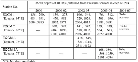
Table 1. Mean depths of RCMs in the deep-sea current meter moorings during each deployment.
Station No. Mean depths of RCMs (obtained from Pressure sensors in each RCM) _______________________________________________________________ 2000 2000-02 2002-03 2003-04 2004-05 EQCM 1
[Equator, 93°E] 156, 290, 484, 991, 2004, 3995
139, 275, 470, 981, 1962, 3971
106, 344, 529, 1024, 2004, 4015
76, 312, 501, 996, 1981, 3991
To be recovered
EQCM 2
[Equator, 83°E] ---- ND, 397, 604, 1093, 2100, 4100
141, 342, 538, 1032, 2026, 4008
139, 339, 534, ND, 2022, 4000
To be recovered
EQCM 3
[Equator, 76°E] ---- ---- 418, 645, 821, 1314,
2311, 4122 ---- ----EQCM 3A
[Equator, 77°E] ---- ---- --- 168, 389, 568, 1059, 2101, 4084
To be recovered
[image:6.595.46.274.651.753.2]During the 2002-03 deployments at 83°E and 76°E locations, the amplitude of the semi-annual wave decreases with depth with highest amplitude of 29 cm/s at 141 m depth at 83°E and lowest amplitude of 10.2 cm/s at 1032 m at 83°E (Table 2). The amplitudes of the semi-annual wave are lower at the 93°E location (during all the 3 deployments), compared to those at the 83°E and 76°E locations. At the 83°E and 76°E locations, one can notice the upward increase of phase from about 800 m to towards surface, indicating the downward propagation of energy associated with the semi-annual wave. This upward phase propagation is clear at 93°E only during January – October 2001 deployment (Table 2). The amplitude and phases of the semi-annual wave fitted to the meridional velocity are also shown in Table 2. The amplitudes are in general smaller compared to the zonal velocity amplitudes, while the phases do not show any trend. The phase of the semi-annual wave fitted to the meridional velocity is almost constant for the 83°E deployment during 2002-03. For the deployment period of 2002-03, the zonal phase increased eastward from 186° at 83°E to 221° at 93°E at the uppermost depth level. This yields an eastward phase velocity of about 80 cm/s which is closer to the speed of the semi-annual Kelvin wave. The depth penetration of the semi-annual wave appears to be deeper at 76°E/77°E and 83°E locations and shallower at 93°E. Further observations and modeling studies are essential to understand this behavior of the semi-annual wave along the equator of the Indian Ocean.
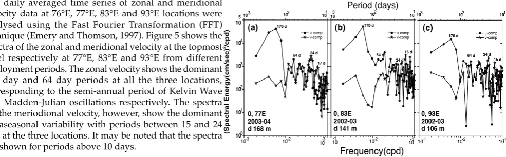
The daily averaged time series of zonal and meridional velocity data at 76°E, 77°E, 83°E and 93°E locations were analysed using the Fast Fourier Transformation (FFT) technique (Emery and Thomson, 1997). Figure 5 shows the spectra of the zonal and meridional velocity at the topmost level respectively at 77°E, 83°E and 93°E from different deployment periods. The zonal velocity shows the dominant 170 day and 64 day periods at all the three locations, corresponding to the semi-annual period of Kelvin Wave and Madden-Julian oscillations respectively. The spectra for the meriodional velocity, however, show the dominant intraseasonal variability with periods between 15 and 24 day at the three locations. It may be noted that the spectra are shown for periods above 10 days.
4. Conclusions
The status of Indian deep-sea current meter moorings along the equator is presented along with the brief results. The observations showed the presence of intraseasonal variability of 10-20 day period. It is noticed that the semi-annual variability is dominant in the central equatorial Indian Ocean and penetrates
to deeper depths, compared to that at 93°E. Further studies are being carried out to analyze the long-term measured current data with various model simulations to identify the variability associated with the Indian Ocean Dipole (Saji et al., 1999). 5. Acknowledgements
The Indian moorings program is funded by the Ministry of Ocean Development (MOD) and the moorings operations were carried out onboard the ORV Sagar Kanya. This is the NIO contribution No. 4188.
References
Emery, W.J., and R. E. Thomson, 1997: Data analysis methods in PhysicalOceanography. Pergaman, Elsevier Science Ltd., UK, 634 p.
Gent, P.R., K. O’Neill, and M.A. Cane, 1983: A model of the semiannual oscillation inthe Equatorial Indian Ocean. J. Phys. Oceanogr., 13, 2148-2160.
McPhaden, M.J., 1982: Variability in the central equatorial Indian Ocean Part I: Oceandynamics. J. Mar., Res., 40, 157-176.
0,93°E
139 m
156 m 106 m
[image:7.595.43.282.74.225.2]months
Figure 3. Long-term variability of zonal (top panel) and meridional (bottom panel) components of current velocity (cm/s) at the equator, 93°E during February 2000 – April 2004.
10-3 10-2 10 -1
100 101 102
103
104
105
103 102 101
10
-3 10-2 10-310-1 10-2 10-1
103 102 101103 102 101
(a)
64 d 24 d
170 d
0, 77E 2003-04 d 168 m
(Spectral Energy(cm/sec
)
2/cpd)
u-comp v-comp
17 d
Period (days)
16 d
(b)
64 d 24 d 170 d
Frequency(cpd)
0, 83E 2002-03 d 141 m
u-comp v-comp
15 d
(c)
64 d 24 d 170 d
0, 93E 2002-03 d 106 m
u-comp v-comp
[image:7.595.321.532.310.497.2]Figure 5. Spectra of zonal (filled circles) and meridional velocity (open stars) at the depths of uppermost Recording Current Meter (RCM) in the moorings at (a) 77°E, (b) 83°E and (c) 93°E. The mean-depth of RCM and the period of deployment are given in the figures. Spectra for periods below 10 days are not shown.
Table 2: The amplitude and phase of the semi-annual variation of zonal and meridional velocity at the mean depths of Recording Current Meters at 93°, 83° and 76°E during 2000-03 in the equatorial Indian Ocean. The phase is referenced from January 1.
Zonal velocity (u) Meridional velocity (v) Mooring
duration Location Mooring Mean depth
(m) Amplitude (cm/s) Phase Amplitude (cm/s) Phase Jan/2000 –
Dec/2000 93°E 156 7.0 309 3.5 22
290 9.8 39 2.4 61
991 4.6 108 1.4 20
Jan/2001 –
Oct/2001 93°E 139 10.1 197 2.4 110
275 6.7 22 1.1 86
470 3.2 307 2.8 137
Apr/2002 –
Mar/2003 93°E 106 13.6 221 1.5 290
Apr/2002 –
Mar/2003 83°E 141 29.2 186 1.1 269
342 13.2 76 2.1 245
538 21.0 44 3.7 244
1032 10.2 334 0.3 79
Aug/2002–
Mar/2003 76°E 418 13.4 101 2.7 176
645 17.7 97 2.5 159
[image:7.595.58.551.569.722.2]Murty, V.S.N., A. Suryanarayana, M.S.S. Sarma, V. Tilvi, V. Fernando, G. Nampoothiri,A. Sardar, D. Gracias, and S. Khalap, 2002: First results of Indian current meter moorings along the equator: Vertical current structure variability at equator, 93°E during February – December 200. Proc. 6th Pan Ocean Remote Sensing Conference, PORSEC 2002, Bali, Indonesia, 1, 25-28.
Prasanna Kumar, S., A. Ishida, K. Yoneyama, M.R. Ramesh Kumar, Y. Kashino, H.Mitsudera, 2005; Dynamics and thermodynamics of the Indian Ocean warm pool in a high-resolution global general circulation model. Deep-Sea Res. Part II, 52; 2031-2047.
Reppin, J., F. Schott, J. Fishcher, and D. Quadfasel, 1999: Equatorial currents andtransports in the upper central Indian Ocean. J. Geophys. Res., 104, 15495-15514.
Saji, N.H., B.N. Goswami, P.N. Vinayachadran, and T. Yamagata, 1999: A dipole mode in the tropical Indian Ocean. Nature, 401, 360-363.
1. Introduction
The Madden-Julian Oscillation (MJO, Madden and Julian 1971, 1972) is known as dominant intraseasonal variability in the tropics. The MJO is an eastward propagating disturbance, occurring primarily during the boreal winter-spring season, with strong atmospheric convection which usually appears at first in the central-eastern equatorial Indian Ocean. Influences of the MJO spread not only within the tropical region but also to the atmospheric and oceanic conditions over the world through interactions with the monsoon (e.g., Yasunari 1979), El Niño (e.g., McPhaden 1999), tropical cyclones (e.g., Maloney and Hartmann 2001), and others. Although previous studies have revealed the various aspects of the MJO, so far there is no definitive explanation on the onset of the MJO convection over the Indian Ocean and associated upper-ocean variability. As for the atmospheric convection itself, recent studies have suggested several key components that have to be clarified by observations. For example, Johnson et al. (1999) demonstrated the trimodal cloud distribution (cumulus, congestus, and cumulonimbus) in the tropics. In particular, it was shown that congestus clouds developed during the suppressed phase of the MJO moistened the mid-troposphere and preconditioned for the active phase with deep convection (Johnson et al. 1999, Kikuchi and Takayabu 2004). Furthermore, the large diurnal cycle in the sea surface temperature in a light wind condition seems to be crucial for the initiation of shallow cumuli and congestus clouds, suggesting the important role of coupling between the atmosphere and the upper ocean in the MJO-convection onset (Slingo et al. 2003). These studies suggest that fine-scale observation from the ocean surface to the entire troposphere is required for better understanding of MJO-convection. The TOGA COARE program in the tropical western Pacific during 1992 and 1993 (Webster and Lukas 1992) was one such observational effort. There are no intensive observations, however, in the Indian Ocean, though fine-scale observations are strongly desired for the study on the initiation of the MJO convection there.
For the upper-ocean variability in the central-eastern tropical Indian Ocean, it has been well known that a strong zonal jet and associated thermocline displacement appear twice
a year during the monsoon transition periods (April-May, and October-November). These are known as the Wyrtki jets (Wyrtki 1973). Using current data from an ADCP mooring at 0°, 90°E, Masumoto et al. (2005), however, demonstrate that intraseasonal disturbances with the 30-50 days period dominate the zonal current in the eastern equatorial Indian Ocean. From their coherence analysis, the intraseasonal variability of zonal currents is considered to be induced by the wind stress between 80°E and 90°E at the periods of 30-50 days. However, details of generation mechanisms for the intraseasonal variability remain unsolved. Thus, it is important to obtain fine resolution data sets to reveal the air-sea interaction processes at the intraseasonal time scale. The data will also be able to be used for validating numerical models and satellite observations, and in turn the models will help in understanding the complex physical processes.
Based on these recent areas of progress, an observational cruise by the R/V Mirai named as MISMO (Mirai Indian Ocean cruise for the Study of the MJO-convection Onset), has been designed to conduct the needed intensive atmospheric and oceanic observations. In the following sections, basic information on the MISMO project will be briefly described.
2. Objectives
The aim of MISMO is to reveal the atmospheric and oceanic features of the central-eastern equatorial Indian Ocean in November, where and when the convection in the MJO is often initiated. Special emphases are put on the following issues: a. Vertical structure of the atmosphere
• Moisture convergence in the lower troposphere
• Variation of vertical profile of atmospheric parameters such as water vapor, divergence field, and clouds
• Development of cumulus convection b. Role of the air-sea interaction
• Diurnal cycle of SST and its difference in behavior before/ after the onset of the MJO
• Variation of ocean surface heat flux c. Oceanic responses to the MJO
• Variation of ocean surface currents accompanied with westerly wind bursts
• Evaluation of warm water and salinity transports
Sengupta, D., Retish Sensan, V.S.N. Murty and V. Fernando, 2004: A biweekly mode inthe equatorial Indian Ocean, J. Geophys. Res., 109, doi:10.1029/2004JC002329.
Unnikrishnan, A.S., S. Prasanna Kumar, G.S. Navelkar, 1997, Large-scale processes inthe upper layers of the Indian Ocean inferred from temperature climatology, J. Mar. Res.: 55(1); 1997; 93-115.
Vinayachandran, P.N., and S.R. Shetye , 1991: The warm pool in the Indian Ocean. Proc. Indian Acad. Sci. (Earth Planet Sci.), 31, 165-175.
Wyrtki, K., 1973, An equatorial jet in the Indian Ocean, Science, 181, 262-264.
MISMO : MIRAI Indian Ocean cruise for the Study of the MJO-convection Onset
Yoneyama, K.1, Y. Masumoto1,2, Y. Kuroda1, M. Katsumata1, and K. Mizuno1
1. Japan Agency for Marine-Earth Science and Technology, Yokosuka, Japan
2. University of Tokyo, Tokyo, Japan.
• Heat budget in the upper-ocean mixed layer 3. Observations
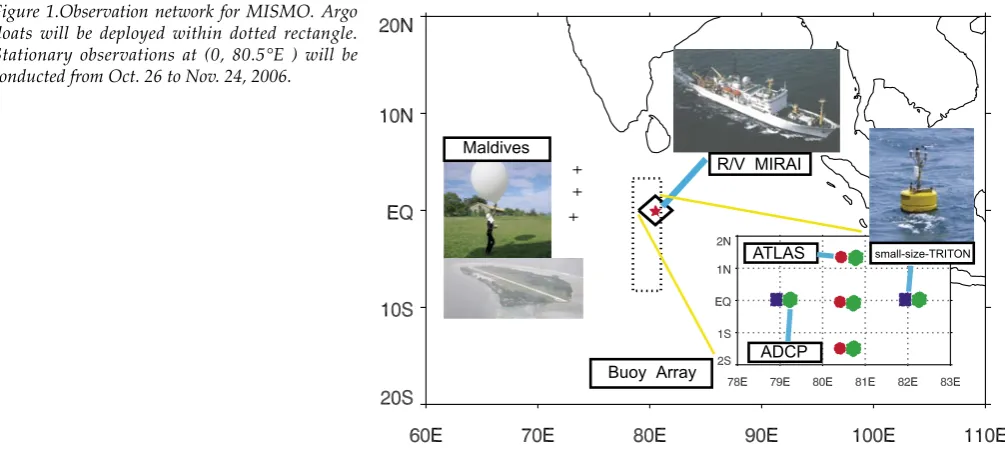
Based on previous studies on the dominant season and location of convective activity in the MJO (e.g., Kemball-Cook and Weare 2001, Zhang and Dong 2004), the intensive observation period and sites will be in October/November and around 80.5°E on the equator, where an ATLAS buoy has been deployed as the intensive flux site by PMEL/NOAA. A proposed observation network during the MISMO is shown in figure 1 (page 16), while a brief summary is as follows.
3.1 R/V Mirai
The main missions of the R/V Mirai are to conduct intensive observations around (0, 80.5°E) for one month and to deploy a mooring buoy array. Since many institutes have been approved to join the cruise through the public invitation process in addition to JAMSTEC and their cooperative institutes, various observations will be carried out during the cruise. Observation items and participating institutes are summarized in Tables 1 and 2.
3.2 Mooring buoy array
A buoy array, consisting of surface and sub-surface moorings, is a major part of the experiment, as it will provide basic upper-ocean conditions as well as ocean surface fluxes. During the MISMO period, newly designed two small-size-TRITON buoys (Fig. 2) will be deployed at (0°, 79°E) and (0°, 82°E), and four sub-surface ADCP moorings will be deployed at (0°,
79°E), (0°, 82°E), (1.5°N, 80.5°E), and (1.5°S, 80.5°E). In addition to these one-month-long moorings, three ATLAS buoys at (1.5°N, 80.5°E), (0°, 80.5°E), (1.5°S, 80.5°E) and a sub-surface ADCP mooring will be replaced before the MISMO cruise by PMEL/NOAA and NIO. The squared buoy array will enable us to calculate the surface heat flux, warm water convergence/ divergence, and, hence, the heat budget in the upper ocean. 3.3 Argo floats
In addition to the standard Argo float 10-day interval sampling from 2000m depth, ten specially programmed Argo floats, which park at 500 m depth and sample once a day, will be deployed along the 80°E line from 8°S to 3°N, to capture the oceanic response to the MJO.
3.4 Land-based sites
To construct the large-scale atmospheric flux array, meteorological measurements will be carried out at three islands, Gan (0.7°S, 73.2°E), Kadhdhoo (1.9°N, 73.5°E) and Hulhule (4.2°N, 73.5°E), in the Republic of Maldives under the cooperation with the Department of Meteorology, Maldives. In addition to the standard surface meteorological measurements, radiosonde observations (2 or 4 times / day) will be conducted at Gan and Hulhule Islands. Furthermore, Doppler radar will be operated at Gan Island.
4. Schedule
The planned schedule of the MISMO cruise (Leg-1 and Leg-2) is as follows. These dates may be subject to change due to various reasons such as weather conditions.
a. Year 2006
• Oct. 4, Depart Sekinehama, Japan • Oct. 15 – 16, Call at Singapore
• Leg-1, Deployment of ADCP moorings, small-size-TRITON buoys, and Argo floats
• Oct. 26 - Nov. 24, Stationary intensive observations at (0, 80.5°E)
• Recovery of ADCP moorings and small-size-TRITON buoys
• Nov. 27 – 28, Call at Male, Maldives
• Leg-2, Recovery/Deployment of TRITON, small-size-TRITON, and ADCP in the Indian Ocean
• Dec. 13 – 14, Call at Singapore
• Leg-3, Recovery / Deployment of TRITON in the western Pacific Ocean
b. Year 2007
• Jan. 16, Arrive at Sekinehama, Japan 5. Concluding remarks
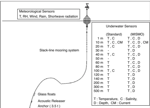
Underwater Sensors
(Standard) (MISMO) 1 m T , C T , C , D 10 m T , C , CM T , C , D , CM 20 m T , C T , C , D 30 m - T , D 40 m T , C T , C , D 50 m - T , D 60 m T T , C , D 80 m T T , C , D 100 m T , C T , C , D
120 m T T , D
140 m T T , D
200 m T T , D
300 m T T , D
500 m T T , D
T : Temperature, C : Salinity, D : Depth, CM : Current Glass floats
Acoustic Releaser Anchor ( 3.5 t ) Meteorological Sensors
T, RH, Wind, Rain, Shortwave radiation
[image:9.595.44.295.69.250.2]Slack-line mooring system
Figure 2.Basic configuration of the small-size-TRITON buoy. A few more depth sensors will be added as standard.
Table 1. Measurement systems on-board the R/V MIRAI
INSTRUMENTS PARAMETERS
5.3-GHz scanning Doppler radar 3-d reflectivity and Doppler velocity
Radiosonde temperature, humidit y, and wind (8 times/day during
IOP)
Ceilometer cloud base height
Tota l sky imager cloud images/fraction in daytime
Surface meteorological sta tion pressure, a ir/sea temperature, humidit y, wind, rain, radia tion
Infrared SST Autonomous Radiometer skin sea surface temperature
Turbulent flux measurement system surface turbulent flux of momentum and latent/sensible hea t
Wind profiler vertica l wind profile in the lower troposphere
Mie Scattering Lidar vertica l profiles of aerosols and clouds
95-GHz Cloud radar vertica l profiles of clouds and rain
Sky radiometer solar radia tion (optica l thickness)
Videosonde images of precipitation and cloud particles within clouds
Radiosonde with hygrometer/ozone sensor
vertica l profile of water vapor and ozone
Ra in sampler rain sampling for stable isotope measurement
Surface water monitoring system sea surface temperature, salinit y, DO, chlorophyll, and pCO2
75-kHz Acoustic Doppler Current Profiler
current vector profile in the upper ocean
CTD with water sampler and
fluorometer
[image:9.595.327.515.602.775.2]vertica l profile of temperature, salinit y, DO, chlorophyll, pH and nutrients (4-8 times /day during IOP
Table 2. Participating institutes for the R/V Mirai cruises
JAPAN JAMSTEC
Na tional Institute for Environmenta l Studies
Hokka ido Univ. Tohoku Univ. Kyoto Univ. Toyama Univ. Osaka Prefecture Univ. Okayama Univ. Yamaguchi Univ.
Global Ocean Development Inc. Marine Works Japan Ltd.
U. S. Univ. of Miami
RMR Co.
International Pacif ic Research Center
During the one-month intensive observation period of MISMO, various atmospheric and oceanic measurements will be carried out at the stationary site and the nearby regions. The data obtained may add new insights to the MJO related variability in both the atmosphere and the ocean and they will be open to the scientific community within a certain period (one or two years). Further information and updates of this experiment can be found at the MISMO web site at http://www.jamstec. go.jp/iorgc/mismo/
References
Johnson, R. H., T. M. Rickenbach, S. A. Rutledge, P. E. Ciesielski, and W. H. Schubert, 1999: Trimodal characteristics of tropical convection. J. Climate, 12, 2397-2418.
Kemball-Cook, S., and B. C. Weare, 2001: The onset of convection in the Madden-Julian oscillation. J. Climate, 14, 780-793. Kikuchi, K., and Y. N. Takayabu, 2004: The development of
organized convection associated with the MJO during TOGA COARE IOP: Trimodal characteristics. Geophys. Res. Lett., 31, L10101, doi:10.1029/ 2004GL019601.
Madden, R. A., and P. R. Julian, 1971: Detection of a 40-50 day oscillation in the zonal wind in the tropical Pacific. J. Atmos. Sci., 28, 702-708.
Madden, R. A., and P. R. Julian, 1972: Description of global-scale circulation cells in the Tropics with a 40-50 day period. J.
Atmos. Sci., 29, 1109-1123.
Maloney, E. D., and D. L. Hartmann, 2001: The Madden-Julian oscillation, barotropic dynamics, and north Pacific tropical cyclone formation. Part I: Observations. J. Atmos. Sci., 58, 2545-2558.
Masumoto, Y., H. Hase, Y. Kuroda, H. Matsuura and K. Takeuchi, 2005: Intraseasonal variability in the upper layer currents observed in the eastern equatorial Indian Ocean. Geophys. Res. Lett., 32, L02607, doi:10.1029/2004GL021896. McPhaden, M. J., 1999: Genesis and evolution of the 1997-98 El
Niño. Science, 283, 950-954.
Slingo, J., P. Inness, R. Neale, S. Woolnough, and G.-Y. Yang, 2003: Scale interactions on diurnal to seasonal timescales and their relevance to model systematic errors. Ann. Geophys., 46, 139-155.
Webster, P. J., and R. Lukas, 1992: TOGA COARE: The Coupled Ocean-Atmosphere Response Experiment. Bull. Amer. Meteor. Soc., 73, 1377-1416.
Wyrtki, K., 1973: An equatorial jet in the Indian Ocean. Science, 181, 262-264.
Yasunari, T., 1979: Cloudiness fluctuations associated with the northern hemisphere summer monsoon. J. Meteor. Soc. Japan,57, 227-242.
Zhang, C., and M. Dong, 2004: Seasonality of the MJO. J. Climate,
The first 1.5 years of INSTANT data reveal the complexities of the Indonesian Throughflow
Gordon A.1, I. Soesilo7, I. Brodjonegoro7, A. Ffield3, I. Jaya8, R. Molcard6, J. Sprintall2, R. D. Susanto1, H. van Aken4, S. Wijffels5, S.
Wirasantosa7
1LDEO, Palisades, NY, USA., 2SIO, La Jolla, CA, USA., 3ESR, Seattle, WA, USA., 4NIOZ, Texel, the Netherlands., 5CSIRO, Hobart, Australia., 6LOCEAN, Paris, France., 7BRKP, Jakarta, Indonesia., 8IPB, Bogor, Indonesia
Corresponding author: [email protected]
The major ocean basins are connected by passages of varied widths and depths. These passages allow for interocean exchange of water properties, which tend to reduce, though not remove, the thermohaline differences between the oceans. Such interocean exchange influences the heat and freshwater budgets of each ocean basin and in so doing represents an important part of the climate system. Most of the interocean exchange routes are at high latitudes, allowing for the establishment of the Antarctic Circumpolar Current and for low salinity surface water flow into the Arctic Sea by way of the Bering Strait. At mid-latitudes there is leakage of subtropical Indian Ocean thermocline water into the South Atlantic around the southern rim of Africa. The Indonesian seas alone allow for an interocean exchange of tropical waters in what is referred to as the Indonesian Throughflow (ITF): a transfer of warm, relatively low salinity Pacific waters into the Indian Ocean. The ITF affects both oceans, though perhaps more so the thermohaline stratification of the smaller Indian Ocean. While the literature of the last 45 years offers a very wide range of annual mean transport values for the ITF, from near zero to 25 x 106 m3/sec,
the more recent estimates narrow the range to 10 ± 5 x 10⁶ m3/sec
with large seasonal and intraseasonal variability (Wijffels and Meyers, 2002; Gordon, 2005).
The ITF stream is fed from the North Pacific thermocline waters, though within the lower thermocline and deeper levels the waters are drawn directly from the South Pacific. The primary inflow passage is Makassar Strait, with the Lifamatola Passage east of Sulawesi the dominant deep-water route. During residence in the Indonesian seas the inflowing Pacific stratification is modified by mixing, with energy derived from dissipation of the powerful tidal currents within the rugged sea floor topography, and by buoyancy flux across the sea-air interface. This results in a unique Indonesian tropical
stratification—one of a strong, though relatively isohaline, thermocline. The Indonesian water is exported into the Indian Ocean via the three major passages within the Sunda archipelago: Timor Passage, Ombai Strait and Lombok Strait. The waters of the ITF are apparent within the thermocline as a cool, low-salinity streak across the Indian Ocean near 12°S (Gordon, 2005) and at intermediate depths as a band of high silicate (Talley and Sprintall, 2005). These ITF waters have no choice but to exit the Indian Ocean within the poleward-flowing western boundary Agulhas Current, though not before mixing and recirculating with ambient Indian Ocean thermocline water and interacting with the monsoonal atmosphere. The ITF acts to flush the Indian Ocean thermocline waters to the south by boosting transport of the Agulhas Current, increasing both the southward ocean heat flux across 20-30°S and the sea-air heat fluxes within the Agulhas Retroflection, over the no-ITF condition (Gordon, 2005).
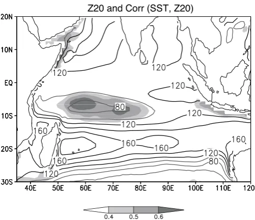
) 0 2 Z , T S S ( rr o C d n a 0 2 Z
Fig. 1. Annual-mean depth of the 20oC isotherm (Z20; contours in m), and correlation between SST and Z20. From Xie et al. (2002). The objectives of INSTANT are: 1. To determine the full depth
velocity and property structure of the Throughflow and its associated heat and freshwater flux; 2. To resolve the annual, seasonal and intraseasonal characteristics of the ITF transport and properties; 3. To investigate the storage and modification of the ITF waters within the internal Indonesian seas, from their Pacific source characteristics to the Indonesian Throughflow water exported into the Indian Ocean; and 4. Contribute to the design of a cost-effective, long-term monitoring strategy for the ITF.
The initial deployment of ten INSTANT moorings was in December 2003 to January 2004 (the 11th, an Ombai mooring, was deployed in August 2003). Approximately 1.5 years later, in June/July 2005, the moorings were recovered and redeployed to acquire an additional 1.5 years of data. The final recovery is scheduled for November/December 2006. A glimpse of the first 1.5 years of INSTANT data is afforded with a composite view of the de-tided along channel speeds for a select mooring and depths within each passage (Fig. 2, page 16).
The along-channel flow within various depth intervals reveals much variability across a wide range of temporal scales, marked with month long periods of significant imbalance between the inflow and export implying substantial convergence and divergence within the interior seas. Makassar Strait along channel speeds are relatively large, with a velocity maximum near 140 m. The southward thermocline speeds are greater towards the latter half of the southeast and northwest monsoons. The estimated Makassar transport is 8 to 9 Sv, about the same or maybe a bit larger than that observed in 1997 during the Arlindo program (Susanto and Gordon, 2005). The highest speeds within the deep water, shown on the >700 m panel of Fig. 2, are in Lifamatola Passage at a current meter ~300 m above the sill depth of ~1940-m. There speeds as high as 0.5 m/sec mark the overflow and descent of Pacific water into the depths of the Seram and Banda Seas. Lombok and Ombai are particularly rich in intraseasonal fluctuations; Makassar and Timor are fairly steady in comparison. Flow into the Indonesian seas is observed within the Lombok and Ombai Straits in late May 2004: a likely cause is a downwelling coastally trapped Kelvin wave propagating eastward along the archipelago as a consequence of a Wyrtki Jet in the equatorial Indian Ocean as was also observed in December 1995 (Molcard et al, 2001) and in May 1997 (Sprintall, et al., 2000). There is a hint of its presence at the Makassar Strait, with a similar 5 day delay as observed in Ombai after northward flows appear in Lombok. In the 350-450 m interval the Makassar flow exhibits the strongest Indian Ocean bound flow, but is matched by westward flow within Ombai within two periods, June-September 2004 and December 2004 to February 2005, coinciding with the peak times of the two monsoon phases.
The first 1.5 years if INSTANT measurements coincide with a weak El Niño, but since the redeployment a weak La Niña phase has ensued. As the ITF is thought to be reduced in El Niño and increased during La Niña, it will be interesting to compare the first 1.5 year record with the final 1.5 year record (though the swing in ENSO phase may not be sufficient to impact of the ITF transport).
Analysis of the INSTANT data in addressing the objectives listed above is a challenge we savor. Each time series is information rich and comparing and interpreting the phase differences between the passages and their varied spectra is an exciting prospect. In particular, comparison of these observations to model results will be a most challenging and interesting exercise. We all look forward to acquiring the full 3 year INSTANT record.
References
Gordon, A.L., 2005. Oceanography of the Indonesian Seas and Their Throughflow. Oceanography18(4): December 14-27 Molcard, R., M. Fieux and F. Syamsudin, 2001. The throughflow
within Ombai Strait, Deep Sea Research I48 1237-1253. Sprintall, J., A.L. Gordon, R. Murtugudde, and R.D. Susanto,
2000. A semiannual Indian Ocean forced Kelvin wave observed in the Indonesian seas in May 1997, Journal of Geophysical Research, 105 (C7), 17217-17230.
Sprintall, J., S. Wijffels, A. L. Gordon, A. Ffield, R. Molcard, R. Dwi Susanto, I. Soesilo, J. Sopaheluwakan, Y. Surachman and H. Van Aken, 2004. INSTANT: A new international array to measure the Indonesian Throughflow. Eos85(39):369. Susanto, R.D. and A. L. Gordon. 2005. Velocity and transport
of the Makassar Strait Throughflow. Journal of Geophysical Research110, Jan C01005, doi:10.1029/2004JC002425. Talley, L.D. and J. Sprintall, 2005. Deep expression of the
Indonesian Throughflow: Indonesian Intermediate Water in the South Equatorial Current, Journal of Geophysical Research, 110 (C10), C10009, doi:10.1029/2004JC002826).
Wijffels, S. E. and G. Meyers, 2002. Interannual Transport Variability of the Indonesian Throughflow and the Role of Remote Wind Forcing. Eos. Trans. AGU, 83(22), West. Pac. Geophys. Meet. Suppl., Abstract OS41B-11, 2002. http:// www.agu.org/meetings/wp02/wp02-pdf/wp02_OS41B. pdf
1. Thermocline dome
This article discusses the recent progress in studying intraseasonal to interannual variability over the South Indian Ocean. The southwest tropical Indian Ocean emerges as a region important for climate variability with high predictability owing to a unique thermocline dome. The dome is centered around 8oS in response to the Ekman pumping between the
southeast trades to the south and weak equatorial westerlies to the north. The shallow thermocline in the dome enables subsurface variability to affect sea surface temperature (SST), as manifested by their high cross-correlation (Fig. 1, page 11). In fact, this thermocline feedback is so strong that Klein et al. (1999) “were unable to match SST anomalies in the southwestern Indian Ocean to any local anomalies in cloud cover or latent heat flux”. The collocation of the mean thermocline dome with the Indian Ocean intertropical convergence zone (ITCZ) suggests that the resultant SST anomalies further influence atmospheric convection. Their collocation is also critical to the formation of the thermocline dome as the intense latent heat release in the Indian Ocean ITCZ generates positive vorticity in the lower troposphere, maintaining an Ekman pumping south of the equator.
2. Interannual Rossby waves
Basin-scale ocean Rossby waves of large amplitudes are observed in the tropical South Indian Ocean (Masumoto and Meyers 1998) in response to El Nino/Southern Oscillation (ENSO) and/or the Indian Ocean dipole (IOD). Propagating into the thermocline dome in the western half of the basin, these subsurface waves induce SST anomalies. Figure 2 shows correlations of Indian Ocean thermocline depth and SST anomalies with an El Nino index. Toward the El Nino’s mature phase (December), wind anomalies in the eastern half of the tropical Indian Ocean excite downwelling Rossby waves in the ocean with characteristic westward propagation. Anomalous winds are easterly on the equator, lifting the thermocline in the east on the equator and on the eastern boundary. Embedded in a basin-wide warming that peaks in February-April following the El Nino, SST anomalies display a positive core that co-propagates with the ocean Rossby waves. These Rossby wave-induced SST anomalies increase local precipitation and tropical cyclone activity, and are collocated with a cyclonic anomalous circulation in the lower troposphere (Xie et al. 2002). Thus, ocean subsurface waves produce a strong response in SST, precipitation, and atmospheric circulation over the thermocline dome. Such atmospheric response to Rossby wave-induced SST anomalies has recently been reproduced in an atmospheric general circulation model (GCM); Annamalai et al. 2005. While earlier studies emphasize the forcing by ENSO, recent partial correlation analyses indicate that the forcing mechanisms for Rossby waves in the tropical Indian Ocean may vary in latitude. Rao and Behera. (2005) and Yu et al. (2005) show that the IOD and ENSO are the major Rossby wave forcing north and south of 10oS, respectively. Yu et al. (2005) suggest that
this variation in Rossby wave forcing is due to the differences in the meridional scale of wind anomalies associated with the IOD and ENSO. The former wind anomalies are more narrowly trapped near the equator than the latter, forcing near-equatorial Rossby waves.
Thermocline dome and climate variability over the tropical South Indian Ocean
Xie S-P.1, J. Luo2, N.H. Saji1, W Yu3
1IPRC/SOEST, Univ. of Hawaii, USA, 2Frontier Research Center for Global Change, Japan, 3First Institute of Oceanography, China
Corresponding author: [email protected]
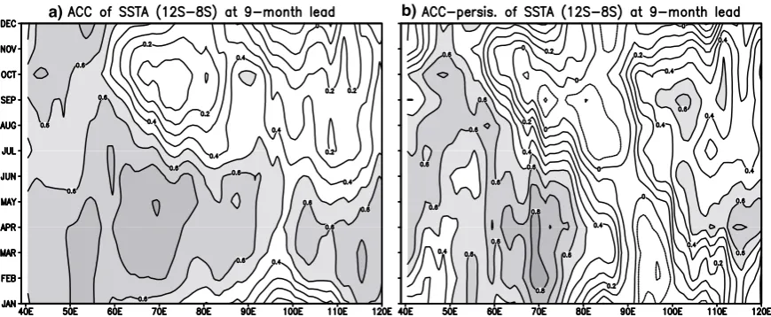
The transit time for these ocean waves across the basin is about one year (Fig. 2), a delay that gives rise to enhanced predictability in a broad region over the tropical South Indian Ocean. Recent seasonal forecast experiments (e.g., Luo et al. 2005) identify the tropical South Indian Ocean as a region of high skills as measured by correlation between the forecast and observations. Figure 3a shows the skills at nine-month lead in the tropical South Indian Ocean of Luo et al.’s (2005) dynamical forecast system based on a fully coupled GCM. Useful skill scores (say, correlation > 0.5) are found across the basin during February-May, and persist in the western basin as late as August. Using the persistence as a baseline, we evaluate the benefits of using a dynamical forecast system. The dynamical system increases the forecast skills over most of the region (Fig. 3b) partly due to an improved ENSO forecast compared to persistence. In the tropical South Indian Ocean, the skill improvements peak in the central basin during February-April and then show a tendency of westward propagation that is characteristics of ocean Rossby waves in Figure 2. Thus, the slow propagation of remotely forced Rossby waves is an important source of predictability.
Modeling the South Indian Ocean Rossby waves and their effects on SST and atmospheric variability remains a challenge. In 17 coupled GCMs submitted for the IPCC fourth assessment report, only a few simulate the ENSO-forced Rossby waves and even fewer capture the co-propagating SST anomalies (Saji et al. 2006a). Forced with observed SST in the tropical Pacific, Huang and Shukla (2006) show that in their coupled model of the Indian Ocean, ENSO-forced Rossby waves exert a discernible influence on SST and the atmosphere as late as during June-August in the year after ENSO peaks. The failure of most IPCC models to simulate this Rossby wave effect may be due to the poor simulation of ENSO, its teleconnection, or the thermocline dome in the South Indian Ocean. This contrasts with the general success of these models in simulating the mean state of the equatorial Indian Ocean, the IOD, and its relationship with ENSO (Saji et al. 2006a).
3. Intraseasonal variability
Nearly free of cloud interference, the Tropical Rain Measuring Mission (TRMM) satellite’s microwave imager (TMI) improves the spatio-temporal sampling of SST observations dramatically over the cloudy tropical Indian Ocean. TMI observations reveal, previously unknown, large intraseasonal SST variability over the tropical South Indian Ocean (Harrison and Vecchi 2001). These intraseasonal anomalies of SST are nearly zonally uniform and occasionally exceed 3oC in range over a large area
(Fig. 4a, page 17). They are preceded by increased atmospheric convective activity and westerly wind anomalies. Analysis of multi-year TMI observations indicates that such intraseasonal SST variability is most pronounced in the tropical South Indian Ocean between 10oS and 5oS over the thermocline dome/ridge,