On the origin of the correlations between the accretion luminosity and emission line luminosities in pre-main-sequence stars

On the origin of the correlations between the accretion luminosity

and emission line luminosities in pre-main-sequence stars

I. Mendigut´ıa,

R. D. Oudmaijer,

E. Rigliaco,

J. R. Fairlamb,

N. Calvet,

J. Muzerolle,

N. Cunningham

and S. L. Lumsden

1_{School of Physics and Astronomy, University of Leeds, Woodhouse Lane, Leeds LS2 9JT, UK}

2_{Swiss Federal Institute of Technology, Department of Physics-Institute for Astronomy, Wolfgang-Pauli-Strasse 27, CH-8093 Zurich, Switzerland} 3_{Department of Astronomy, University of Michigan, 830 Dennison Building, 500 Church Street, Ann Arbor, MI 48109, USA}

4_{Space Telescope Science Institute, 3700 San Martin Drive, Baltimore, MD 21218, USA}

Accepted 2015 July 8. Received 2015 July 6; in original form 2015 May 12

A B S T R A C T

Correlations between the accretion luminosity and emission line luminosities (LaccandLline) of

pre-main-sequence (PMS) stars have been published for many different spectral lines, which are used to estimate accretion rates. Despite the origin of those correlations is unknown, this could be attributed to direct or indirect physical relations between the emission line formation

and the accretion mechanism. This work shows that all (near-UV/optical/near-IR)Lacc–Lline

correlations are the result of the fact that the accretion luminosity and the stellar luminosity (L_∗)

are correlated, and are not necessarily related with the physical origin of the line. Synthetic and

observational data are used to illustrate how theLacc–Llinecorrelations depend on theLacc–L∗

relationship. We conclude that because PMS stars show theLacc–L∗correlation immediately

implies thatLaccalso correlates with the luminosity of all emission lines, for which theLacc–

Llinecorrelations alone do not prove any physical connection with accretion but can only be

used with practical purposes to roughly estimate accretion rates. When looking for correlations

with possible physical meaning, we suggest thatLacc/L∗andLline/L∗should be used instead of

LaccandLline. Finally, the finding thatLacc has a steeper dependence onL∗ for T Tauri stars

than for intermediate-mass Herbig Ae/Be stars is also discussed. That is explained from the magnetospheric accretion scenario and the different photospheric properties in the near-UV.

Key words: accretion, accretion discs – line: formation – methods: miscellaneous – stars: pre-main sequence – stars: variables: T Tauri, Herbig Ae/Be.

1 I N T R O D U C T I O N

The disc-to-star accretion rate is one of the most important pa-rameters driving the evolution of pre-main-sequence (PMS) stars. However, it is difficult to directly measure the mass accretion rate, for which indirect empirical methods are necessary to estimate it. A widely used method exploits the fact that the accretion luminos-ity (Lacc) correlates with the luminosity of various emission lines (Lline). Despite the unknown origin of these correlations, they are being used to quickly estimate accretion rates. TheLacc–Lline empir-ical correlations have been derived using samples of PMS stars by comparing their accretion luminosities, mostly obtained from the UV excess and line veiling, with the emission line luminosity (see e.g. Muzerolle, Hartmann & Calvet1998b; Dahm2008; Herczeg & Hillenbrand2008; Fang et al. 2009; Rigliaco et al. 2012, and references therein). Currently, dozens of near-UV–optical–near-IR

_{E-mail:[email protected]}

spectral lines have been found to correlate withLacc for classical T Tauri (TT) stars (for instance, the hydrogen Balmer and Paschen series, HeI, OI, Na ID and CaIItransitions, Brγ, etc; see e.g. Alcal´a et al.2014, hereafterAL14). The correlations of the accre-tion luminosity with several of these lines have been extended both to the sub-stellar and the intermediate-mass Herbig Ae/Be (HAeBe) regimes (Mohanty, Jayawardhana & Basri 2005; Donehew & Brittain2011; Mendigut´ıa et al.2011,2013; Rigliaco et al.2011).

Apart from the observational effort involved to look for addi-tional emission lines that could serve as accretion tracers, several investigations aim to provide physical links between some of the spectral transitions and the accretion process, which would ex-plain the origin of theLacc–Llinecorrelations. In a nutshell, either the lines are directly tracing the accreting region (e.g. Muzerolle, Calvet & Hartmann1998c; Muzerolle, Hartmann & Calvet1998a; Kurosawa, Harries & Symington2006; Rigliaco et al.2015), or they trace the accretion indirectly, by probing the accretion-powered outflows and winds (e.g. Hartigan, Edwards & Ghandour 1995; Edwards et al. 2006; Kurosawa, Romanova & Harries 2011;

2015 The Authors

at University of Leeds on March 30, 2016

http://mnras.oxfordjournals.org/

Kurosawa & Romanova2012). The correlation with forbidden lines like [OI] (6300 Å) exhibited by HAeBes (Mendigut´ıa et al.2011) is more difficult to explain, as this line is not identified with ac-cretion/winds but rather with the surface layers of the circumstellar discs (Acke, van den Ancker & Dullemond2005). A further chal-lenge to the various explanations of the origin of the Lacc–Lline correlations is that the variations in the accretion rate as measured from the UV excess do not generally correlate with the observed changes in the line luminosities (Nguyen et al.2009; Mendigut´ıa et al.2011,2013; Costigan et al.2012). However, time delays be-tween different physical processes could be present (Dupree et al. 2012).

On the other hand, the accretion luminosity is also found to correlate with the luminosity of the central star (L_∗). TheLacc–L∗ correlation extends over∼10 orders of magnitude inLacc, and∼7 orders of magnitude in L_∗, covering all optically visible young stars from the sub-stellar to the HAeBe regime (see e.g. Clarke & Pringle2006; Natta, Testi & Randich2006; Tilling et al.2008; Mendigut´ıa et al.2011; Fairlamb et al.2015, and references therein). Based on a statistical analysis, Mendigut´ıa et al. (2011) tentatively suggested that the correlation between the accretion luminosity and the luminosity of several emission lines in HAeBe stars could be driven by the common dependence of both luminosities on the stellar luminosity.

The main goal of this paper is to demonstrate the equivalence of theLacc–LlineandLacc–L∗correlations. In particular, we aim to show that all (near-UV, optical and near-IR)Lacc–Llinecorrelations in PMS stars are driven by the relationship between the stellar lumi-nosity and the accretion lumilumi-nosity, and that therefore the accretion luminosity necessarily correlates with the luminosity of all spectral lines regardless of their physical origin. Section 2 introduces and partially re-analyses theLacc–L∗correlation in PMS stars. Section 3 shows the expression that links theLacc–L∗relationship with the

Lacc–Llinecorrelations. The inter-dependence between both types of correlations is illustrated in Section 4 using both synthetic data and observational data from the literature. Some implications from all the previous analysis are included in Section 5. Finally, Section 6 summarizes our main conclusions.

2 T H E Lacc–L∗ C O R R E L AT I O N

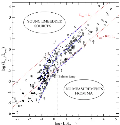
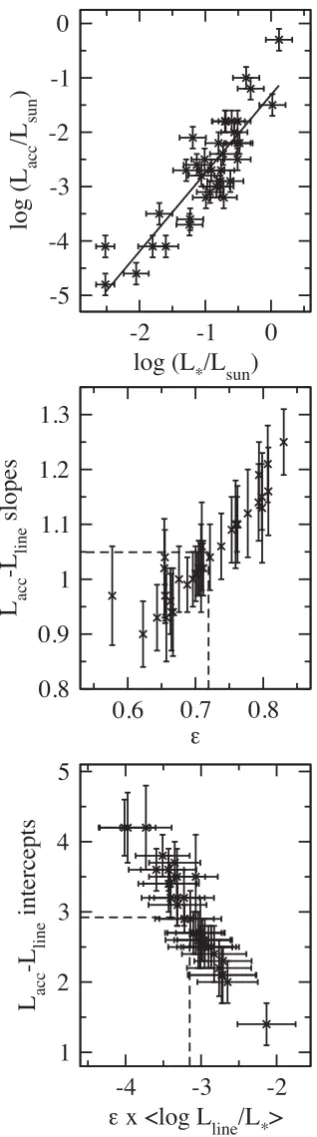
A representative example of the empirical correlation between the accretion and stellar luminosities1_{is shown in Fig.1. It includes} data from the literature for very low mass TTs and sub-stellar objects/companions (log (L_∗/L) < −1.25), TTs (−1.25< log (L∗/L)<0.75), late-type HAeBes (0.75<log (L∗/L)<2.25), and early-type HAeBes (log (L_∗/L)>2.25). The sources belong to different star-forming regions. The graph shows thatLaccincreases withL_∗, with a relation steeper for the TTs than for the HAeBes.

According to Clarke & Pringle (2006) and Tilling et al. (2008), the upper bound of theLacc–L∗correlation (Lacc∼L∗) is the con-sequence of sample selection effects; the luminosity of most stars above that limit is dominated by accretion and these objects are in a younger, embedded phase without an optically visible photosphere. The lower bound (Lacc∼0.01L∗, mainly for objects withL∗>L) is limited by accretion detection thresholds (symbols with vertical bars in Fig.1). The physical origin of theLacc–L∗correlation is the

1_{Its counterpart, the relationship between mass accretion rate and stellar} mass, can be derived from theLacc–L∗correlation using PMS tracks (see e.g. Clarke & Pringle2006).

Figure 1. Lacc–L∗correlation for sub-stellar objects and TTs in different star-forming regions (crosses; with vertical bars for upper limits; Natta et al. 2006; Herczeg & Hillenbrand2008, and references therein), four (sub-) stellar/planetary companions around PMS stars (squares; Close et al.

2014; Zhou et al.2014), the Lupus sample fromAL14(dark triangles) and HAeBes (circles; with vertical bars for upper limits; Mendigut´ıa et al.2011; Fairlamb et al.2015). The red diagonal dotted lines indicateLacc=L∗and Lacc=0.01L∗. The three blue diagonal dashed lines represent the accretion luminosities expected from MA modelling for Balmer excesses of 0.70, 0.12 and 0.01 mag (top, mid and bottom lines, respectively). The vertical dotted line indicates the stellar luminosity at which the Balmer jump becomes apparent in the photospheric spectra (see also Fig.2). [A colour version of this figure is available in the online journal.]

subject of active debate. This topic is not analysed here but we re-fer the reader to several related works (e.g. Padoan et al.2005; Alexander & Armitage 2006; Dullemond, Natta & Testi 2006; Vorobyov & Basu2008; Ercolano et al.2014). Instead, our contribu-tion below deals with the observed change in the slope of theLacc–L∗ correlation between the TT and the HAeBe stars (Mendigut´ıa et al. 2011; Fairlamb et al.2015).

We constructed a sample of artificial stars representing the TT and HAeBe regime by using synthetic models of stellar atmo-spheres (Kurucz1993). The properties of each object are provided in Table1. Columns two and three show the stellar luminosity and ef-fective temperature. From these, the stellar radii was derived, span-ning between 0.7 and 4 R(column 4). The stellar masses (column 5) were derived assuming logg= 4, and cover the 0.2–6 M range. Magnetospheric accretion (MA) shock modelling was car-ried out for each star by adding (blackbody) accretion contributions to the photospheric (Kurucz) spectra (see e.g. the reviews in Calvet, Hartmann & Strom2000; Mendigut´ıa2013). Two representative examples are presented in Fig. 2 (left-hand panel). The shock model was applied following the usual recipes for both the TTs and HAeBes, and we refer the reader to Calvet & Gullbring (1998); Mendigut´ıa et al. (2011) and Fairlamb et al. (2015) for further de-tails. Three different values for the UV excess in the Balmer region of the spectra (from∼3500 to 4000 Å, as defined in Mendigut´ıa et al. 2013) were modelled for each object assuming typical values for

at University of Leeds on March 30, 2016

http://mnras.oxfordjournals.org/

acc line

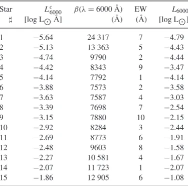
Table 1. Sample of artificial stars. Stellar parameters and accretion luminosities from MA. Columns two to five show the stellar luminosity (logarithmic scale, from the in-tegrated Kurucz model atmospheres), effective temperature, stellar radius and mass. Columns six to eight show the MA accretion luminosities (logarithmic scale) corre-sponding to a minimum (m), typical (t) and maximum (M) Balmer excess of 0.01, 0.12 and 0.70 mag, respectively.

Star L∗ T∗ R∗ M∗ (Lacc)m (Lacc)t (Lacc)M [log L] (K) (R) (M) [log L] [log L] [log L]

1 −1.25 3500 0.65 0.15 −4.85 −3.75 −2.84

2 −1.00 4000 0.66 0.16 −4.28 −3.17 −2.26

3 −0.75 4500 0.70 0.18 −3.64 −2.53 −1.61

4 −0.50 5000 0.75 0.20 −3.10 −1.99 −1.04

5 −0.25 5500 0.83 0.25 −2.62 −1.50 −0.53

6 0.00 6000 0.93 0.31 −2.20 −1.08 −0.08

7 0.25 6500 1.05 0.40 −1.85 −0.74 0.29

8 0.50 7000 1.21 0.53 −1.57 −0.45 0.58

9 0.75 7500 1.41 0.72 −1.36 −0.25 0.76

10 1.00 8000 1.65 0.99 −1.13 −0.02 0.98

11 1.25 8500 1.95 1.38 −0.89 0.22 1.21

12 1.50 9000 2.32 1.95 −0.64 0.47 1.46

13 1.75 9500 2.78 2.80 −0.40 0.72 1.71

14 2.00 10 000 3.34 4.05 −0.15 0.97 1.96

15 2.25 10 500 4.04 5.93 0.10 1.22 2.22

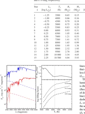
Figure 2. Left-hand panel: MA modelling of a typical Balmer excess (0.12 mag) for two representative stars with stellar temperatures of 7500 (blue) and 5500K(red). The photospheric (Kurucz) spectra, the contribution from accretion and the total flux obtained from the combination of the previous are represented by the dotted, dot–dashed and solid lines, respectively. The fluxes are as they would be measured at the stellar surface. Right-hand panels: photosphericU−Bcolours (taken from Kenyon & Hartmann1995) characterizing the Balmer region of the spectrum (top) and filling factors necessary to reproduce a Balmer excess of 0.01, 0.12 and 0.70 mag (bottom) using MA, versus the stellar temperature. The vertical dotted line indicates the stellar temperature at which the Balmer jump becomes apparent in the photospheric spectra (see also Fig.1). [A colour version of this figure is available in the online journal.]

the inward flux of energy carried by the accretion columns (1012_erg cm2_s−1_{) and the disc truncation radius (5R}

∗): a ‘maximum’ excess (0.70 mag), whose corresponding accretion contribution isLacc∼L∗ forL_∗≥L; a ‘minimum’ excess (0.01 mag) representative of the observational limit, and whose corresponding accretion contribu-tion isLacc∼0.01L∗forL∗≥L; and finally, a ‘typical’ excess in-between the two previous (0.12 mag). The resulting accretion lu-minosities are shown in the last three columns of Table1. These are plotted versus the correspondingL_∗values (blue diagonal dashed

lines in Fig.1), matching the overall distribution of data. We note that excesses larger than 0.70 mag could still be measured for the less luminous sources (L_∗≤L) without reaching the upper bound (Lacc∼L∗).

The fact that the accretion luminosity increases with the stellar luminosity is a natural consequence of MA shock modelling. This is illustrated in the left-hand panel of Fig.2. When the same excess (flux ratio between the solid and dotted lines) is observed in stars of different stellar luminosity, the most luminous stars (blue dotted line) must necessarily have a larger accretion contribution (dot– dashed lines). In order to understand the different slope in theLacc–

L∗correlation for TT and HAeBe stars, it is important to recall that the accretion contribution, and thereforeLacc, is proportional to both the temperature of the accretion columns (Tcol) and the filling factor (f), which represents the fraction of the stellar surface covered by the accretion shocks. Variations inTcol andfmove the accretion-generated continuum excess along the wavelength axis and flux axis, respectively. The typical value forTcolis∼104K across the TT and HAeBe regimes. Therefore, the excess peaks close to the Balmer region for both types of star. However, their photospheric spectra (i.e. when accretion is not present) are significantly different in that region. The Balmer jump becomes visible only for stars with log (L∗/L)≥0.25 (i.e.T∗≥6500 K).2_{This makes the spectra of stars} with spectral types F and earlier more similar between them in the Balmer region than for later spectral types. Fig.2(top-right panel) illustrates the case; the photosphericU–Bcolour characterizing the Balmer region shows a steep dependence on the stellar temperature for cool stars, and flattens for hotter objects. Therefore, in order to reproduce a given Balmer excess, TTs require larger variations in the accretion luminosity than the ones that HAeBes need, for which the slopeLacc/L∗decreases from the TT to the HAeBe regime. The accretion luminosity changes are mainly affected by variations in the filling factor. This is shown in Fig.2(bottom-right panel), where the filling factors that are needed to reproduce the minimum, typical and maximum model excesses are plotted against

2_{The Balmer jump disappears again in O stars withT}

∗≥30 000 K.

at University of Leeds on March 30, 2016

http://mnras.oxfordjournals.org/

the stellar temperature. The change of slope in this panel occurs at the temperature where the Balmer jump appears (∼6500 K), which corresponds to the stellar luminosity when the slope of theLacc–

L∗correlation changes (log (L∗/L)∼0.25). It is noted that we have applied basic MA modelling without considering aspects like the chromospheric contribution to the spectra of TT stars (Manara et al.2013) or changes in the disc truncation radius depending on the stellar mass regime (Muzerolle et al.2004; Mendigut´ıa et al. 2011; Cauley & Johns-Krull 2014). These factors could change the accretion estimates by less than 0.5 dex, without significantly affecting the modelled results in Figs1and2.

In summary, the observed difference in theLacc–L∗correlation between TTs and HAeBes can be explained from the MA scenario and the differences in the near-UV stellar properties between both types of stars. However, we emphasize that the overallLacc–L∗ cor-relation is not a mere consequence of the MA shock modelling but most probably reflects a deeper physical relationship between both parameters (see e.g. the references at the beginning of this section). For example, the specific slopes shown by different samples in dif-ferent environments (see e.g the Lupus sample with solid triangles in Fig.1) cannot simply be explained from MA. Moreover, theLacc–L∗ correlation seems to arise also in embedded, younger sources, when the accretion luminosities are estimated from a variety of methods (Beltr´an & de Wit, in preparation). Regardless of the underlying physical origin of theLacc–L∗correlation, for the rest of the paper it will be enough to remind that this arises whenever a significant sample of PMS stars is considered.

3 T H E AC C R E T I O N – S T E L L A R - L I N E L U M I N O S I T Y R E L AT I O N

The relation between the accretion and stellar luminosities is usually expressed in the literature asLacc ∝ Lb_∗. This can also be written as a linear expression, which is a reasonable approach when the TT and HAeBe regimes are studied separately. For a given star, we will assume thatLaccandL∗can then be related by

log

Lacc L

=a+b×log

L∗ L

, (1)

withaandbconstants that depend on the star considered. When a sample of stars is studied,aandbrepresent the intercept and the slope of a linear fit to the data. This situation will be analysed in Section 4.

The luminosity of a spectral line can be computed by multiply-ing the line equivalent width (EW) and the luminosity (per unit wavelength) of the adjacent continuum (Lc_λ):

Lline=Lc_λ×EW=

_α· EW β

×L∗, (2)

with α the (dimensionless) excess of the (dereddened) contin-uum with respect to the photosphere at the wavelength of the line (α=Lc_λ/Lλ∗>=1), andβthe ratio between the total stellar luminos-ity and the stellar luminosluminos-ity at that wavelength (β=L_∗/L_λ∗ 1, in units of wavelength). The stellar luminosity in the second term of equation (2) was introduced in equation (1), obtaining

log

Lacc L

=A+B×log

Lline L

, (3)

which is again a linear expression, with

A=a−b×log

Lline L∗

,

B =b, (4)

Table 2. Sample of artificial stars. Continuum and line prop-erties. Columns two to five list the luminosity of the con-tinuum at 6000 Å (logarithmic scale), the ratio between the total, star+accretion, luminosity and the stellar luminos-ity at 6000 Å, a random EW of an hypothetical emission line assigned to each star (between 1 and 10 Å), and its corresponding luminosity at 6000 Å (logarithmic scale). Star Lc₆₀₀₀ β(λ=6000 Å) EW L6000

[log LÅ] (Å) (Å) [log L]

1 −5.64 24 317 7 −4.79

2 −5.13 13 363 5 −4.43

3 −4.74 9790 2 −4.44

4 −4.42 8343 9 −3.47

5 −4.14 7792 1 −4.14

6 −3.88 7573 2 −3.58

7 −3.63 7587 4 −3.03

8 −3.39 7698 7 −2.54

9 −3.15 7880 10 −2.15

10 −2.92 8284 3 −2.44

11 −2.69 8773 6 −1.91

12 −2.48 9603 8 −1.58

13 −2.27 10 581 4 −1.67

14 −2.07 11 723 1 −2.07

15 −1.86 12 905 6 −1.08

whereLline/L∗ = αEW/β, is the line to stellar luminosity ratio. Therefore, if the accretion luminosity of a given star can be de-rived from its stellar luminosity through equation (1), then the same accretion luminosity can be recovered from the luminosity of any emission line through equations (3) and (4), withAandBconstants that depend on the star and the line considered. Equations (1) and (3) are equivalent because both express a common dependence of the accretion luminosity on the stellar luminosity (equation 2).

4 T H E D E P E N D E N C E O F T H E Lacc–Lline C O R R E L AT I O N S O N T H E Lacc–L∗ R E L AT I O N

In this section, we use both synthetic and empirical data to illustrate the dependence of theLacc–Llinecorrelations on theLacc–L∗relation. Our first analysis provides a simple qualitative example on how the shape of theLacc–L∗relationship has a strong effect on theLacc–Lline correlations. We use the sample of artificial stars introduced in the previous section (see the first five columns of Table1). The Kurucz models were used to calculateLc_λandβat 6000 Å, whose values are presented in columns two and three of Table2. Random EWs (between 1 and 10 Å, column four) are assigned to each object. These range in EW is representative of emission lines with inter-mediate strength such as the CaIIor OItransitions. The luminosity of an artificial emission line at 6000 Å (column five) can then be obtained from equations (2).

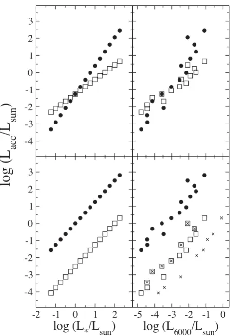
The top-left panel of Fig.3shows two differentLacc–L∗linear relations assumed for the sample. Both have the same intercept but a different slope. The reverse is shown in the bottom-left panel, in which the slope is kept constant and the intercept varies. The right-hand panels show the corresponding accretion luminosities versus the luminosity of the artificial line at 6000 Å. TheLacc–Lline correlations follow the changes introduced in theLacc−L∗relation, varying their slopes and intercepts. The range in the EW used only affects the scatter of theLacc–Llinecorrelation, but this is ultimately determined by theLacc −L∗relation. As introduced in Section 3,

at University of Leeds on March 30, 2016

http://mnras.oxfordjournals.org/

acc line

Figure 3. Results for the sample of artificial stars, showing how changes in the assumedLacc–L∗correlation (left-hand panels) have an effect on the Lacc–Llinerelation (right-hand panels) by changing the slope (top panels) and the intercept (bottom panels) of the former correlations. The crosses in the bottom-right panel represent the line luminosities obtained from a wider EW range, when the EWs≥5 Å in column 5 of Table2are multiplied by a factor 10.

the contribution of the continuum to the line luminosity dominates over the EW, and both the continuum and the accretion luminosities are correlated with the stellar luminosity. In order to illustrate this, the EW range was increased multiplying by 10 all the EWs≥5 Å in column 4 of Table2, and keeping the rest unmodified. This range in EW is representative of a strong emission line such as Hα. The new line luminosities are plotted with crosses in the bottom-right panel of Fig.3, showing that for wider (narrower) EW ranges, the scatter in theLacc–Lline correlation increases (decreases), but the correlation remains.

Before using real data from the literature to illustrate how the

Lacc–Llineempirical correlations are driven by theLacc–L∗relation, the equations described in the previous section have to be slightly modified. There, the values ofLacc were given by equations (1) and (3), wherea, b, Aand Bdiffer depending on the individual star and spectral line. In practice, the values for the slopes and intercepts of these equations are estimated using linear regression fitting, which provide uniqueaandbvalues for a given sample of stars, as well as uniqueAandBvalues for a given spectral line. In this case it can be shown (see Appendix A) that the slopes and intercepts of theLacc–L∗and theLacc–Llineempirical correlations are

related by

A∼a−b× ×

logLline

L∗

;

B =b× ;

= rline×σ∗ r∗×σline

∼1,

(5)

where A, a;B, and brepresent the intercepts and slopes of the

Lacc–L∗ andLacc–Lline correlations, as derived from least-squares linear regression fitting,logLline/L∗the mean (logarithmic) line to stellar luminosity ratio,r∗andrlinethe correlation coefficients of theLacc–L∗andLacc–Llinelinear fits, andσ∗andσlinethe standard deviations of the log (L_∗/L) and log (Lline/L) values.

In short, when the empiricalLacc–L∗andLacc–Llinecorrelations are compared, equations (5) should be used instead of equations (4). These are slightly modified by including the parameter, which accounts for the fact that the empirical correlations are in practice derived from (least-squares) linear fitting.3

We use the observational data inAL14to illustrate the depen-dence of theLacc–Llineempirical correlations on theLacc −L∗ re-lation. These authors studied a sample of 36 low-mass TTs in the Lupus star-forming region, for which they derived stellar parame-ters, accretion rates from the UV excess, andLacc–Llineempirical correlations for dozens of emission lines in the spectral range from the near-UV to the near-infrared. To our knowledge, this work con-tains the largest number of spectral lines for which this type of correlations are derived. Another advantage is that for each star the accretion luminosity and the luminosity of all spectral lines were derived from the same spectrum, avoiding the problem of variabil-ity. In addition, all the stars are located at a similar distance, which guarantees that the correlations were not artificially stretched when the fluxes are multiplied by the squared distances to derive the (ac-cretion and line) luminosities. Therefore, we consider theLacc−

L∗andLacc–Llinecorrelations inAL14as representative for simi-lar correlations provided in the literature (see e.g the references in Section 1).

The top panel of Fig.4shows the accretion and stellar lumi-nosities of the stars studied byAL14. The observed trend is best fitted by log (Lacc/L)∼ −1.3+1.4×log (L∗/L) (solid line). The slopes and intercepts of theLacc–Llineempirical correlations derived byAL14(see their table 4), which are exactly recovered by equations (5), are plotted in the mid and bottom panels of Fig.4 versus and × logLline/L∗, respectively. The mid panel shows that the slopes of theLacc–Llineempirical correlations are a factor smaller than the slope of theLacc–L∗correlation shown by the sample. As expected from equations (5), the Lacc–Lline empirical correlations become steeper when increases, eventually reaching a slope of∼1.4 for =1. The bottom panel shows the expected linear decrease of the intercepts of theLacc–Llinecorrelations with the ( -modified) line to stellar luminosity ratio. Equations (5) also imply that the typical (mean) slope of allLacc–Llinecorrelations is given by the slope of theLacc−L∗correlation of the sample, cor-rected by the mean value of ;B =b× . Similarly, it can be derived that the mean intercept of theLacc–Llinecorrelations is given byA =a−b× × logLline/L∗. The two previous relations are also observed in theAL14data, the mean values indicated with

3_{Linear regression fits obtained from methods different than the usual} least-squares are not considered in this work. The parameter should be eventually modified if other linear regression methods are used.

at University of Leeds on March 30, 2016

http://mnras.oxfordjournals.org/

Figure 4. Based on results inAL14. Top panel: accretion versus stellar luminosity. The best linear fit is log (Lacc/L)∼ −1.3+1.4×log (L∗/L) (solid line). Mid and bottom panels: slopes and intercepts of the Lacc– Llineempirical correlations versus the parameter (mid-panel) and the -modified mean (logarithmic) line to stellar luminosity ratio (bottom panel). The dashed lines indicate the mean values for thexandyaxis, related from the slope and intercept of the top panel correlation by:y =1.4x(mid panel), andy = −1.3–1.4x(bottom panel).

the dashed lines perpendicular to both axis in the mid and bottom panels of Fig 5.

In summary, the analysis of both a sample of artificial stars and representative empirical data shows that theLacc–Llinecorrelations are driven by the underlyingLacc−L∗relation shown by the sample of stars under study.

5 C O N S E Q U E N C E S

The first consequence of the analysis in the previous sections is that the fact that PMS stars show theLacc−L∗correlation imme-diately implies thatLaccalso correlates with the luminosity of any (near-UV–optical–near-IR) emission line, regardless of the physical origin of the spectral transition. Indeed, it even correlates with the luminosity of a randomly general artificial emission line (right-hand panels of Fig.3). As mentioned earlier, the scatter of theLacc–Lline correlations increases when the lines’ EWs exhibit a larger range. A similar effect occurs for stars with strong excess at short, UV, wavelengths and long, IR, wavelengths. For lines observed at these short and long wavelengths, the ratioαEW/β(i.e. the line to stel-lar luminosity ratio; equation 2) becomes significant, which could make theLacc–Llinecorrelations much more scattered or eventually disappear.

For the other lines, theLacc–Llinecorrelations are mainly deter-mined by theLacc −L∗dependence shown by the sample under analysis. The intercepts and slopes provided in the literature for the

Lacc − L∗correlation (aandbin equation 1) vary depending on the sample of stars considered (Fairlamb et al.2015, and references therein). Based on those works, a conservative observational limit is−2.5≤a≤0, 0.8≤b≤2. Consequently (see equations 4 and 5), the slopes of allLacc–Llineempirical correlations should also range in between∼0.8 and 2, whereas the intercepts should all be>0 and decrease as the mean line to stellar luminosity ratio increases. These predictions agree with allLacc–Lline published correlations based on observational data, to our knowledge. Interestingly, if two samples of stars show a different slope in their correspondingLacc–

L_∗ correlations, then the slopes of theLacc–Lline ones are simply related viaB∼B×(b/b) (assuming that the factors in equation (5) are roughly similar in both samples). This effect has already been observed. Mendigut´ıa et al. (2011) reported a slight decrease in the slope of theLacc–L∗correlation of a sample of 34 HAeBe stars with respect to TTs (see also Fig.1and Fairlamb et al.2015). As discussed there, the slopes of theLacc–Llineempirical correlations for the three lines studied (Hα, [OI] (6300 Å), and Brγ) also show a similar decrease.

That Lacc correlates withLline is ultimately due to a common dependence of both luminosities on the stellar brightness. Because of this and the reasons above, theLacc–Llinecorrelations alone cannot be seen as proof for either a direct or indirect physical connection between the spectral transitions and the accretion process. However, they are still useful expressions that can be applied to easily derive accretion luminosities without the need for sophisticated modelling of the UV excess. A basic measurement of a line luminosity suffices. Given that both observationalLacc–Lline andLacc–L∗ correlations show a roughly similar scatter (around±1 dex inLacc), the latter can also be used to easily derive accretion rates from the stellar luminosity.

Analogously, since Lline necessarily correlates withL∗ (equa-tion 2), correla(equa-tions betweenLlineandL∗alone cannot be taken as a possible physical link between the spectral transition and the stellar luminosity (see also Natta et al.2014). By extension, the luminosi-ties of two different emission lines should also correlate with each

at University of Leeds on March 30, 2016

http://mnras.oxfordjournals.org/

acc line

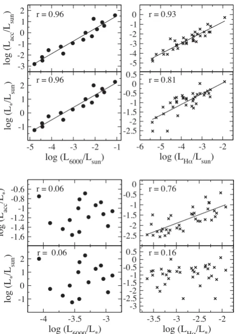
Figure 5. Comparison between different luminosities normalized by the solar and the stellar luminosity, as indicated in the axes’ labels. The left-hand panels refer to the sample of artificial stars in Table2, and the right-hand panels to real observations fromAL14. Linear regression fits are overplotted for those cases with large enough correlation coefficients (r>0.50;r-values indicated in each panel).

other because of the common dependence on the stellar luminosity. Again, exceptions are possible for lines at short/long wavelengths in stars with strong excesses (see e.g. Meeus et al.2012).

In order to infer from correlations possible physical links involv-ing the luminosity of a spectral line or the accretion luminosity, it is necessary to get rid of the common dependence of both parameters on the stellar luminosity. This can be done by dividingLlineandLacc byL_∗. Fig.5(top panels) shows theLacc–Lline correlation for the sample of artificial stars from Table2and a givenLacc−L∗relation, and the intrinsic correlation between the stellar and line luminosi-ties. However, the bottom-left panels show that bothLacc/L∗ and

L_∗do not correlate withLline/L∗, as expected from an artificial line created with random EWs. The right-hand panels of the same figure show the results of the same exercise using real data fromAL14. As expected, the Hαluminosity correlates with both the accretion and stellar luminosities, which as we have discussed has no possible physical interpretation. In contrast with the previous example, in this case the Hαline to stellar luminosity ratio is still correlated with the accretion to stellar luminosity ratio but not with the stellar luminosity itself, supporting the idea that this line is mainly driven by accretion and not by the stellar brightness.

With this perspective in mind, we have confirmed that all line luminosities provided inAL14 correlate with each other, as ex-pected. We also have checked that when the line luminosities are

normalized by the stellar luminosities, some correlations remain while others disappear, indicating the presence or absence of a physical link between the different spectral transitions. For exam-ple, for Hαand Brγ the correlation is not only between their line luminosities but also between their line to stellar luminosity ratios, suggesting a common physical origin for both transitions. In con-trast, despite the fact that the luminosities of the HeII(4686 Å) and the CaII(8498 Å) lines correlate, their line to stellar luminosities do not show a significant correlation, suggesting a different physical origin.

Finally, when the generalLacc−L∗correlation analysed in Sec-tion 2 is transformed intoLacc/L∗versusL∗, no trend is shown either for the whole sample or for specific samples like the Lupus objects inAL14. The vast majority of the objects have 0.01≤Lacc/L∗≤1 (diagonal dotted lines in Fig.1) for all stellar luminosity bins. The typical value ofLacc/L∗is 0.1, which corresponds to the modelled, typical Balmer excess of 0.12 mag. For the less luminous sources (L_∗<L), smallerLacc/L∗ratios can still be obtained from the same Balmer excess detection limit. As discussed in Section 2, this is the expected consequence of the MA scenario and the photospheric properties of the stars in the near-UV.

It is beyond the scope of this work to carry out a detailed study on physical correlations involving stellar, line and accretion lumi-nosities. Instead, we have provided several examples to suggest that correlation analysis aiming to infer physical consequences should useLline/L∗andLacc/L∗and not simplyLlineandLacc.

6 S U M M A RY A N D C O N C L U S I O N S

TheLacc−L∗empirical correlation in PMS stars has been partially re-analysed taking into account the newly available accretion rates for HAeBes. Despite the physical origin of theLacc−L∗correlation remains subject to debate, the observed change of slope from the TT to the HAeBe regime can be understood from the MA scenario and the near-UV photospheric properties of the stars.

We have shown that the fact that PMS stars show theLacc−L∗ correlation immediately implies thatLaccalso correlates with the lu-minosity of any (near-UV, optical, near-IR) emission line, regardless of the physical origin of the spectral transition. The overallLacc–

Llinetrends are mainly governed by theLacc–L∗correlation shown by the sample of stars under analysis. In particular, the slopes of the

Lacc–Llineempirical correlations should typically be between∼0.8 and 2 for all spectral lines, which are the observational limits for the slope of theLacc–L∗relation. The intercepts also depend on the

Lacc–L∗correlation, all of which are>0 and increasing as the line to stellar luminosity ratio decreases.

Despite the fact that the Lacc–Lline correlations alone do not constitute an indication of any direct or indirect physical link be-tween the spectral transitions and accretion, they are a useful tool to easily derive estimates of the accretion rates. The Lacc − L∗ correlations can be used for the same purpose. Similarly, cor-relations between stellar and line luminosities, or between dif-ferent line luminosities, do not indicate a physical relation be-tween the parameters involved. Instead, we suggest that the line to stellar and accretion to stellar luminosity ratios should be used when investigating the possible physical origin of the various correlations.

AC K N OW L E D G E M E N T S

The authors sincerely acknowledge A. Natta, W.J. de Wit and M. Beltr´an for the fruitful discussions that have served to improve the

at University of Leeds on March 30, 2016

http://mnras.oxfordjournals.org/

contents of this manuscript, as well as the anonymous referee for her/his useful comments.

R E F E R E N C E S

Acke B., van den Ancker M. E., Dullemond C. P., 2005, A&A, 436, 209 Alcal´a J. M. et al., 2014, A&A, 561, A2 (AL14)

Alexander R. D., Armitage P. J., 2006, ApJ, 639, L83 Calvet N., Gullbring E., 1998, ApJ, 509, 802

Calvet N., Hartmann L., Strom S. E., 2000, in Mannings V., Boss A. P., Russell S. S., eds, Protostars and Planets IV. Univ. Arizona Press, Tucson, AZ, p. 377

Cauley P. W., Johns-Krull C. M., 2014, ApJ, 797, 112 Clarke C. J., Pringle J. E., 2006, MNRAS, 370, L10 Close L. M. et al., 2014, ApJ, 781, L30

Costigan G., Scholz A., Stelzer B., Ray T., Vink J. S., Mohanty S., 2012, MNRAS, 427, 1344

Dahm S. E., 2008, AJ, 136, 547

Donehew B., Brittain S., 2011, AJ, 141, 46

Dullemond C. D., Natta A., Testi L., 2006, ApJ, 645, L69 Dupree A. K. et al., 2012, ApJ, 750, 73

Edwards S., Fischer W., Hillenbrand L., Kwan J., 2006, ApJ, 646, 319 Ercolano B., Mayr D., Owen J. E., Rosotti G., Manara C. F., 2014, MNRAS,

439, 256

Fairlamb J. R., Oudmaijer R. D., Mendigut´ıa I., Ilee J. D., van den Ancker M. E., 2015, MNRAS, in press

Fang M., van Boekel R., Wang W., Carmona A., Sicilia-Aguilar A., Henning Th., 2009, A&A, 504, 461

Hartigan P., Edwards S., Ghandour L., 1995, ApJ, 452, 736 Herczeg G. J., Hillenbrand L. A., 2008, ApJ, 681, 594 Kenyon S. J., Hartmann L., 1995, ApJS, 101, 117 Kurosawa R., Romanova M. M., 2012, MNRAS, 426, 2901

Kurosawa R., Harries T. J., Symington N. H., 2006, MNRAS, 370, 580 Kurosawa R., Romanova M. M., Harries T. J., 2011, MNRAS, 416,

2623

Kurucz R. L., 1993, SYNTHE Spectrum Synthesis Programs and Line Data, Kurucz CD-ROM 18. Smithsonian Astrophysical Observatory, Cambridge, MA

Manara C. F. et al., 2013, A&A, 551, A107 Meeus G. et al., 2012, A&A, 544, A78 Mendigut´ıa I., 2013, Astron. Nachr., 334, 129

Mendigut´ıa I., Calvet N., Montesinos B., Mora A., Muzerolle J., Eiroa C., Oudmaijer R. D., Mern B., 2011, A&A, 535, A99

Mendigut´ıa I. et al., 2013, ApJ, 776, 44

Mohanty S., Jayawardhana R., Basri G., 2005, ApJ, 626, 498 Muzerolle J., Hartmann L., Calvet N., 1998a, AJ, 116, 455 Muzerolle J., Hartmann L., Calvet N., 1998b, AJ, 116, 2965 Muzerolle J., Calvet N., Hartmann L., 1998c, ApJ, 492, 743

Muzerolle J., D’Alessio P., Calvet N., Hartmann L., 2004, ApJ, 617, 406 Natta A., Testi L., Randich S., 2006, A&A, 452, 245

Natta A., Testi L., Alcal´a J. M., Rigliaco E., Covino E., Stelzer B., D’Elia V., 2014, A&A, 569, A5

Nguyen D. C., Scholz A., van Kerkwijk M. H., Jayawardhana R., Brandeker A., 2009, ApJ, 694, L153

Padoan P., Kritsuk A., Norman M., Nordlund Å., 2005, ApJ, 622, L61 Rigliaco E., Natta A., Randich S., Testi L., Covino E., Herczeg G., Alcal

J. M., 2011, A&A, 526, L6

Rigliaco E., Natta A., Testi L., Randich S., Alcal J. M., Covino E., Stelzer B., 2012, A&A, 548, A56

Rigliaco E. et al., 2015, ApJ, 801, 31

Tilling I., Clarke C. J., Pringle J. E., Tout C. A., 2008, MNRAS, 385, 1530 Vorobyov E. I., Basu S., 2008, ApJ, 676, L139

Zhou Y., Herczeg1 G. J., Kraus A. L., Metchev S., Cruz K. L., 2014, ApJ, 783, L1

A P P E N D I X A : R E L AT I O N B E T W E E N T H E

Lacc–Lline A N D Lacc–L∗ L I N E A R R E G R E S S I O N

C O R R E L AT I O N S

Consider a sample ofN stars for which measurements of accre-tion and stellar luminosities [log (Lacc/L)1,..., log (Lacc/L)N; log

(L_∗/L)1,..., log (L∗/L)N)] are available. A linear fit to the data

provides an expression that links both variables through

log

Lacc L

=a+b×log

L∗ L

, (A1)

withaand bconstants representing the intercept and the slope, which from least-squares linear regression are given by

b=r∗×

_σ acc σ∗ ; a= log Lacc L

−b×

log L∗ L , (A2)

wherer∗is the correlation coefficient (∼1 for well correlated data), andσacc,σ∗;logLacc/L, andlogL∗/Lthe standard devia-tions and the means of the log (Lacc/L)iand log (L∗/L)ivalues,

respectively.

Similarly, if for the same sample of stars there are additional measurements of the luminosity of a given emission line [log (Lline/L)1,..., log (Lline/L)N], then a linear fit provides

log _L

acc L

=A+B×log _L

line L

, (A3)

withAandBconstants given by least-squares linear regression

B=rline×

_σ acc σline ; A= log Lacc L

−B×

log Lline L , (A4)

where the correlation coefficient, standard deviations, and means now refer to the [log (Lacc/L)i, log (Lline/L)i] values.

The standard deviationσacccan be found in the expression for

bof equation (A2), and then introduced in the expression forBof equation (A4), providing the expression relating the slopes of the

Lacc–L∗andLacc–Llinelinear correlations:

B= ×b;

= rline×σ∗ r∗×σline

. (A5)

On the other hand, the mean valuelogLacc/Lcan be found in the expression fora of equation (A2), and introduced in the expression forAof equation (A4). Also considering equation (A5), the expression that relates both intercepts is

A=a−b× ×

log Lline L∗ − 1− × log L∗ L . (A6)

The third term could been neglected ((1− )/ ∼0) compared with the two other terms in the previous equation.

This paper has been typeset from a TEX/LA_{TEX file prepared by the author.}

at University of Leeds on March 30, 2016

http://mnras.oxfordjournals.org/