Predictions of Heat Transfer and Flow Circulations in Differentially Heated Liquid Columns With Applications to Low-Pressure Evaporators

White Rose Research Online URL for this paper: http://eprints.whiterose.ac.uk/85931/

Version: Accepted Version Article:

Panesar, JS, Heggs, PJ, Burns, AD et al. (2 more authors) (2015) Predictions of Heat Transfer and Flow Circulations in Differentially Heated Liquid Columns With Applications to Low-Pressure Evaporators. Heat Transfer Engineering, 36 (14-15). 1177 - 1191. ISSN 0145-7632

https://doi.org/10.1080/01457632.2015.994459

[email protected] https://eprints.whiterose.ac.uk/

Reuse

Unless indicated otherwise, fulltext items are protected by copyright with all rights reserved. The copyright exception in section 29 of the Copyright, Designs and Patents Act 1988 allows the making of a single copy solely for the purpose of non-commercial research or private study within the limits of fair dealing. The publisher or other rights-holder may allow further reproduction and re-use of this version - refer to the White Rose Research Online record for this item. Where records identify the publisher as the copyright holder, users can verify any specific terms of use on the publisher’s website.

Takedown

If you consider content in White Rose Research Online to be in breach of UK law, please notify us by

Predictions of Heat Transfer and Flow Circulations in Differentially Heated Liquid

Columns with Applications to Low Pressure Evaporators

Jujar S. Panesar1, Peter J. Heggs2, Alan D. Burns1, Lin Ma1, Stephen J. Graham3

1

Energy Technology Innovation Initiative, University of Leeds, Leeds, LS2 9JT

2

School of Chemical and Process Engineering, University of Leeds, Leeds, LS2 9JT

3

National Nuclear Laboratory Ltd, Chadwick House, Warrington Road, Warrington, WA3

6AE

Address correspondence to Professor Peter Heggs, School of Chemical and Process

ABSTRACT

Numerical computations are presented for the temperature and velocity distributions of two

differentially heated liquid columns with liquor depths of 0.1 m and 2.215 m respectively. The

temperatures in the liquid columns vary considerably with respect to position for pure

conduction, free convection and nucleate boiling cases using 1D thermal resistance

networks. In the thermal resistance networks the solutions are not sensitive to the type of

condensing and boiling heat transfer coefficients used. However these networks are limited

and give no indication of velocity distributions occurring within the liquor. To alleviate this

issue, 2D axisymmetric and 3D CFD simulations of the test rigs have been performed. The

axisymmetric conditions of the 2D simulations produce unphysical solutions; however the full

3D simulations do not exhibit these behaviours. There is reasonable agreement for the

predicted temperatures, heat fluxes and heat transfer coefficients when comparing the boiling

case of the 1D thermal resistance networks and the CFD simulations.

This work was undertaken by the University of Leeds and National Nuclear Laboratory Ltd

as part of our on-going support of Sellafield Ltd’s operations. The work was funded by the

EPSRC, National Nuclear Laboratory Ltd and Sellafield Ltd/NDA through an EPSRC CASE

award.

INTRODUCTION

In the UK, during refuelling of nuclear reactors, fuel bundles are removed and stored

in spent fuel ponds to allow short lived fission products to decay. After a suitable length of

storage, the fuel bundles are sent to the Magnox or Thorp facilities at the Sellafield nuclear

reprocessing site (hereinafter referred to as Sellafield), depending on the type of reactor from

which they originate. The spent fuel is dissolved in nitric acid where solvent extraction and

other processes occur [1] (for further details of highly active waste management at Sellafield

the reader is referred to Upson [2]). One of the products of this process is highly active liquor

which is sent to several low pressure (0.1 bar) kettle type evaporators currently in operation at

Sellafield. The purpose of the evaporators is to boil the highly active liquor, thus reducing its

water content and causing it to become more concentrated with a much lower volume. The

evaporation of highly active liquor occurs prior to vitrification into solid glass and long term

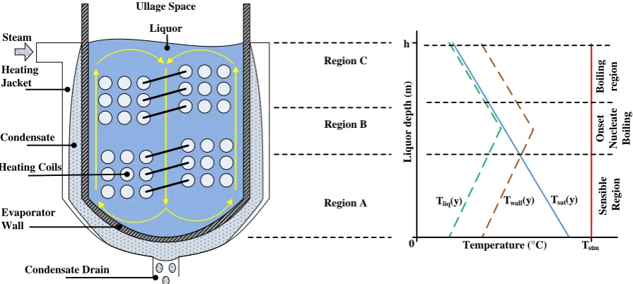
storage. The Sellafield evaporators depicted in Figure 1 operate by condensing dry saturated

steam inside an external heating jacket and inside a number of helical coils which are

submerged within the highly active liquor.

The liquor fill height of the Sellafield evaporators is approximately 2 m from the base.

The saturation temperature of the liquor is greatest at the base of the evaporator due to the

contribution of the hydrostatic head, and lowest at the free surface. Hence it is hypothesised

that a subcooled boiling region may exist with respect to liquor depth inside the Sellafield

evaporators as shown in Figure 1. In region A, sensible heating increases the temperature of

the bulk liquor which approaches the saturation temperature. In this region liquor circulations

are prevalent due to natural convection. In region B, the conditions are met for the onset of

nucleate boiling. The local wall superheat produces vapour bubbles at nucleation sites which

will condense back into the liquor; or detach and become carried away with the circulations

and bulk liquor are at saturated conditions where boiling takes place. At the walls, vapour

bubbles are continuously formed and detached which escape at the free surface. At the free

surface flashing occurs which contributes to the generation of vapour.

During the evaporation process crystalline salt solids are formed which may settle on

the bed of the evaporator or stay in suspension due to the density variations within the liquor.

The presence of these crystalline salt solids may affect the position of boiling and circulations

within the liquor.

The highly active liquor is highly corrosive. The lifetime of the various heating

components are limited by the rate of corrosion of the heat transfer surfaces, which is a

function of the temperature at the heat transfer surface [3]. Hence accurate predictions of

temperature and flow distributions inside the Sellafield evaporators are highly desirable.

It is difficult to monitor heat transfer, boiling and multiphase flow components of the

Sellafield evaporators and to directly relate the results to the predictions of internal surface

temperatures and flows. To address this issue National Nuclear Laboratory Ltd have

commissioned two small scale non-radioactive test rigs to characterise the transport

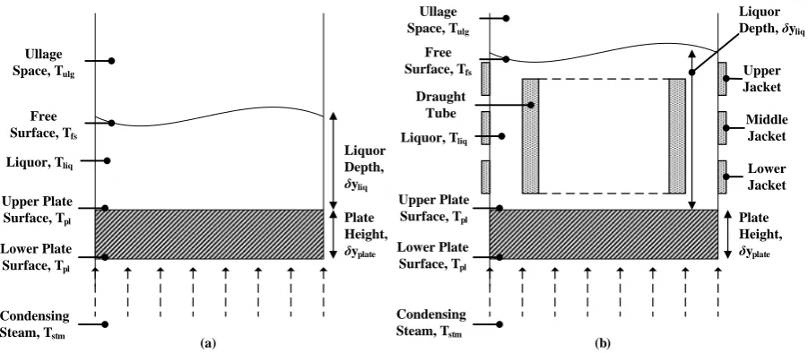
phenomena occurring within the Sellafield evaporators, illustrated in Figure 2. The two test

rigs have a diameter of 0.1 m and metal base plate thickness of 0.02 m, but different fill

heights of 0.1 and 2.215 m (hereinafter referred to as the short and tall test rigs respectively).

The fill height for the short test rig has a 1:1 ratio between the fill height and vessel width,

which is close to the aspect ratio found in the Sellafield evaporators. The fill height of the tall

test rig is similar to that found in the Sellafield evaporators, and has been chosen such that the

hydrostatic pressure dependence of heat transfer and the fluid circulations occurring in the

tall test rig can be studied. The tall test rig also has two features not found in the short test rig:

evaporators; (ii) three circumferential heating jackets which provide additional heating to the

liquor.

The test rigs operate by condensing saturated steam on the lower surface of the

stainless steel base plate, where the upper surface of the base plate is in contact with the

liquid column. In addition, for the tall test rig, the three heating jackets are set to temperatures

of 50, 60 and 70 °C for the upper, middle and lower heating jackets respectively. The ullage

pressure and temperature is maintained at a saturation pressure and temperature of 0.1 bar

and 45.8 °C respectively.

Heat transfer across the boundaries of the liquid column causes density variations in

the liquid which lead to flow circulations. The position of the boiling within the liquid

column greatly affects the circulations. Depending upon the pressure head of the liquid

column, boiling can occur on the top surface of the base plate, or close to the free surface of

the liquid column. In the latter case, the internal circulation will be equivalent to an

unconstrained thermosyphon reboiler situation [4], with the generation of vapour greatly

increasing the circulation. The temperature distributions within the liquid column will

significantly affect the temperatures of the heat transfer surfaces, which are essential

requirements for the estimation of rates of corrosion of the surfaces. It is an essential

requirement to understand where boiling will occur with respect to liquor depth.

Previous Studies

Previous studies have been conducted to obtain a more accurate understanding of free

convection, boiling and condensation inside the test rigs. Geddes et al. [3] performed an

iterative calculation procedure based on the precedence ordering technique [5] to estimate the

heat flux and temperature distribution over the length of the internal coils of the Sellafield

number of correlations for the boiling heat transfer coefficient. The largest disagreement for

the coil surface was 9°C when using different correlations for the boiling heat transfer

coefficient.

Wakem et al. [1] presented an overview of the heat transfer modelling work that was

undertaken between National Nuclear Laboratory Ltd and Sellafield Ltd to remove

conservative predictions on the condition of the Sellafield evaporators. The paper presents a

thermal resistance methodology to estimate the wall superheat. It was estimated that surface

temperatures were high enough to initiate nucleate boiling at the heat transfer surface that

was under investigation. A CFD investigation was also conducted, modelling one of their

experimental test rigs as a 2D rectangular slice through the centre, and using water as the

liquor in a single phase convection simulation. The velocity and circulatory behaviour of the

simulated liquor was a function of plate and wall temperatures. In addition to the simulation

of the experimental test rigs, a preliminary CFD investigation of heat and fluid flow localised

at the base of the Sellafield evaporators was conducted.

Perry and Geddes [6] used Nusselt’s analytical approach of condensation on a vertical

flat surface [7] and extended it to account for the condensation on the outer surface of the

toroidal section of the Sellafield evaporators (i.e. the external heating jacket as shown in

Figure 1). Using the same assumptions as those used by Nusselt [7], the analytical

condensation model by Perry and Geddes [6] attempts to account for increasing condensate

thickness down the walls. The model was presented in terms of a local heat transfer

coefficient. The model was compared to a mean condensation heat transfer coefficient and

showed general agreement.

The aims of this paper are to provide a greater understanding of the heat transfer and

fluid circulations in the test rigs, and to develop simple numerical models to predict these

behaviours. As CFD simulations can become computationally prohibitive with respect to

complexity, available resources and time, a simple technique is desirable to estimate the

temperatures and heat fluxes occurring in the test rigs without using CFD. The temperatures

and heat fluxes can be compared to CFD models to ascertain if agreement between the two

methods exists. Additionally fluid circulations are difficult to monitor directly inside the test

rigs when using experimental methods. CFD simulations are used to estimate the fluid

circulations occurring inside the test rigs. Furthermore this paper aims to clarify if symmetry

boundary conditions can be used to model buoyancy driven flow within the test rigs.

THERMAL RESISTANCE INVESTIGATION

The temperatures and heat fluxes in the test rigs are predicted by thermal resistance

networks which accommodate condensation below the base plate and conduction through the

base plate, and three conditions in the liquor above the base plate by pure conduction, free

convection and nucleate boiling. This involved generating a system of equations which

describes the transport of heat through thermal resistances.

Several assumptions have been included in the thermal resistance investigation: the heat

transfer analysis is 1D in the vertical y direction; two temperatures in the system are known

(Dirichlet boundary conditions) which are the steam and ullage temperatures, or the steam

and liquor saturation temperatures. For all three cases the common steam temperature is

126.9 _°C, and for the pure conduction and free convection cases the ullage temperature is

45.8 °C corresponding to the ullage saturation pressure of 0.1 bar. For the nucleate boiling

rigs respectively. The liquor is water and no fouling exists on the heat transfer surfaces. For

the pure conduction case for the liquor, the thermal conductivity of water is constant

throughout the liquid column. For the free convection case it is assumed that no boiling

occurs, and the liquor is divided by two rotating convection cells between the upper plate and

free surface. For the boiling case it is assumed that nucleate boiling occurs at the heat transfer

surface. Radiation heat transfer is ignored and the side walls are adiabatic. The thermal

resistance networks of the three cases are illustrated in Figure 3. Due to the non-linear

correlations for the condensation, convection and boiling heat transfer coefficients that are

used the values of the unknowns are solved for iteratively, using a numerical program written

in MatLab which used the Newton Raphson iterative technique. Curve fitted correlations are

used for the thermophysical properties of water and steam as a function of temperature [8].

Test Case (a): Pure Conduction Through The Liquor

Figure 3 (a) represents the thermal resistance network diagram for the pure

conduction through the liquor. There are four resistances in sequence described by equations

(1) to (4). Equation (1) describes the condensation resistance underneath the base plate.

Equations (2) and (3) describe the conduction resistances through the base plate and liquor

respectively. Equation (4) describes the free convection resistance in the ullage region. The

four unknown values to be determined are the heat flux, lower plate temperature, upper plate

temperature and free surface temperature.

(1)

(2)

(3)

Two correlations for the condensation heat transfer coefficient in equation (1) are used

independently of each other: (i) the analytical Nusselt [7] heat transfer coefficient for the

condensation of vapours on vertical flat plates; and (ii) the empirical Gerstmann and Griffith

[9] heat transfer coefficient for the condensation of vapours underneath downward facing

surfaces. The Nusselt heat transfer coefficient takes the form as shown in equation (5).

N� (5)

The enthalpy of vaporisation in Nusselt’s correlation is replaced with an augmented enthalpy

of vaporisation [10] which takes into effect the condensate subcooling as shown in equation

(6).

(6)

The Gerstmann and Griffith [9] condensation heat transfer coefficient is formulated in terms

of a Rayleigh number in the following equation:

N� _RaRa _RaRa (7)

The Nusselt and Rayleigh numbers in equation (7) are defined as follows:

N� (8)

Ra (9)

The free convection heat transfer coefficient in the ullage region in equation (4) is

treated as a hot surface facing upward from the free surface (or a cold surface facing

downward) [11] as shown in equation (10).

N� Ra Ra ��

The Rayleigh number is defined as:

Ra G��� (11)

Test Case (b): Free Convection In The Liquor

The network for free convection in Figure 3 (b) has five sequential thermal resistances.

The bottom two are identical to the previous case which are condensation on the lower

surface of the base plate and conduction through the base plate described by equations (1)

and (2) respectively. The next two resistances in Figure 3 (b) represent free convection in the

liquor. It is assumed there are two rotating convection cells inside the liquid column which

are treated as a hot surface facing upward from the upper plate as shown in equation (12), and

a cold surface facing downward from the free surface as shown in equation (13) [11], and

hence the heat transfer coefficients are treated by equation (10). The free convection

resistance in the ullage region is also identical to the previous case described by equation (4).

Hence the governing equations for the free convection case are equations (1), (2), (4), (12)

and (13), and the five unknown values that are to be determined are the heat flux, lower plate

temperature, upper plate temperature, mid liquor temperature and free surface temperature.

(12)

(13)

Test Case 3: Nucleate Boiling In The Liquor

The network diagram for nucleate boiling in Figure 3 (c) has only three resistances. The

thermal resistances described by equations (1) and (2) in the pure conduction case remain

applicable for the nucleate boiling case. Equation (14) describes nucleate boiling occurring at

equations (1), (2) and (14), and the three unknown values to be determined are the heat flux,

lower plate temperature and upper plate temperature.

(14)

It is assumed that nucleate boiling occurs at the upper plate surface, where the

saturation temperature corresponds to the liquor depth. The saturation temperature is

determined using Antoine’s vapour pressure correlation as shown in equation (15), using the

constants by Linstrom and Mallard [12], which are 5.20389 bar, 1733.926 °C and -39.485 °C

for A, B and C respectively. The saturation temperatures are 51.7 and 70.4 °C for the short

and tall test rigs respectively, corresponding to 0.1 bar ullage pressure and the liquid column

hydrostatic pressure head. At the free surface it is assumed the liquor flashes to vapour.

lo� lo� (15)

Six individual correlations for the nucleate boiling heat transfer coefficient are used in

equation (14). The first correlation used for the boiling heat transfer coefficient is the Forster

and Zuber [13] correlation defined as:

(16)

The second and third correlations used are the Mostinskii [14] and Bier et al. [15]

correlations, which share the same expression for heat transfer coefficient shown in equation

(17), however differ by their definition for the pressure correction factor as shown in

equations (18) and (19) respectively.

(17)

(18)

The fourth and fifth correlations used are the Cooper [16] and Rohsenow [17] boiling heat

transfer coefficients, shown in equations (20) and (21) respectively.

lo� (20)

(21)

In the Rohsenow correlation in equation (21) C is defined as:

(22)

The exponent n is taken as unity, which is valid for boiling water (and 1.7 for other fluids)

[18]. The value of the surface finish is dimensionless, and values can be obtained from

Collier and Thome [19]. For this investigation its value is taken as 0.0080. The sixth

correlation used is that by Gorenflo and Kenning [20] as shown in equation (23).

(23)

For boiling water, the pressure correction factor is calculated using equation (24).

(24)

The exponent n for boiling water is determined as follows:

(25)

The values for the reference heat transfer coefficient, surface roughness and heat flux are

5600 W/m2·°C, 0.4 m, and 20,000 W/m2 respectively. Hewitt et al. [18] report that there are

large deviations between the boiling heat transfer coefficients, and no general guidelines can

be provided on the boiling correlation that should be used. The wall superheat required to

initiate nucleate boiling for each test case is calculated using the Davis and Anderson

(26)

Thermal Resistance Investigation Results

The results from the thermal resistance investigation for the three cases (case (a) pure

conduction through the liquor, case (b) free convection in the liquor and case (c) nucleate

boiling in the liquor) are tabulated in Tables 1, 2 and 3 respectively. The overall heat transfer

coefficients are orders of magnitude lower in cases (a) and (b) than in case (c). This is

because the values of the free convection heat transfer coefficient in the ullage region are

small which reduces the overall heat transfer coefficient. Hence the free convection thermal

resistance in the ullage region is the limiting resistance in cases (a) and (b). In case (c) the

limiting thermal resistance is conduction heat transfer through the base plate. However all

three cases share the same conduction thermal resistance through the base plate, and in all

three cases their resistance values are the same. To reduce the conduction thermal resistance,

and consequently increase the heat flux through the system the thickness of the base plate

should be reduced, or alternatively a base plate material with a higher thermal conductivity

should be used.

In case (c) with the exception of the Cooper correlation, all boiling heat transfer

coefficients are in agreement, despite their very diverse formulations. Rohsenow et al. [20]

report that the square root of the molecular weight in the Cooper correlation is an

oversimplification which can yield significant errors in the value of the boiling heat transfer

coefficient.

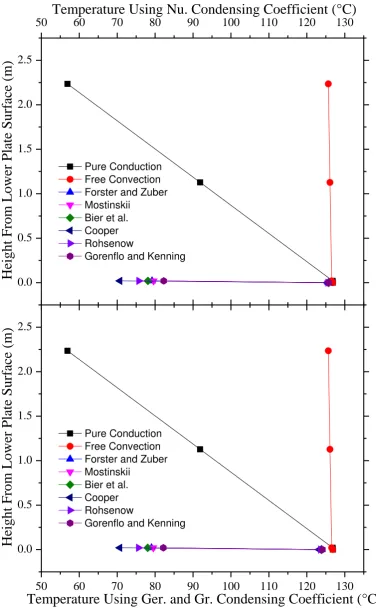
Figures 4 and 5 are plots of the temperature variation with height, starting at the lower

plate surface up to the free surface for cases (a) and (b), and up to the upper plate surface for

case (c) – boiling of the liquor. For case (c) the temperature difference between the lower and

correlations used. For all boiling heat transfer coefficients, the temperature difference

between the upper plate surface and liquor saturation exceeds the calculated wall superheat

required to initiate nucleate boiling when calculated using equation (26).

There is very little variation in the solutions when using either the Nusselt or

Gerstmann and Griffith condensing correlations on both test rigs. This is because the thermal

resistance due to conduction in the baseplate removes any sensitivity of the solution to using

different condensation or boiling heat transfer coefficients.

CFD INVESTIGATION

A limitation of the thermal resistance investigation is that it does not provide

information regarding the circulation of liquor, such as liquor velocities and direction.

Instead, assumptions had to be made based on the number of convection cells occurring

within the liquid column (free convection cases) or the position of boiling inside the system

(nucleate boiling cases). Furthermore the thermal resistance investigation was only 1D hence

further information is required of the heat transfer and circulations inside the test rigs.

CFD simulations are performed of the two test rigs and their results compared to the

results from the thermal resistance investigation. For the short test rig, simulations on 2D

axisymmetric and a full 3D geometry is performed to ascertain if axisymmetric conditions are

a viable alternative to a full 3D simulation. Furthermore a full 3D simulation is performed on

the tall test rig. The commercial code Ansys CFX v14.0 is used to perform the CFD

simulations.

Upon start-up the thermal behaviour of the liquor in the test rigs will be dominated by

pure conduction for a finite time, until a critical Rayleigh number is achieved wherein free

CFD cases is when phase change occurs in the bulk liquor. During this time a pseudo steady

state condition may exist where flow features may repeat periodically.

Boundary Conditions

The free surface and ullage region is modelled as an opening with pressure and

temperature equal to the ullage pressure and temperature which are 0.1 bar and 45.8 °C

respectively. In the short and tall test rigs, ambient heat loss from the non-jacketed side walls

and from the non-insulated sides of the base plate is taken into consideration. At the vertical

sides of the baseplate, the correlation recommended by Churchill and Chu [22] as shown in

equation (27) is used. The ambient outside temperature is taken as 26.9 °C.

N� (27)

At the non-jacketed walls of the liquid columns an average heat transfer coefficient is used

which takes the wall glass thickness, into consideration as shown in equation (28).

(28)

In the tall test rig the top, middle and bottom heating jackets are set to fixed wall

temperatures of 50, 60 and 70 °C respectively. In both test rigs, condensation underneath the

baseplate is not directly modelled; instead the Nusselt [7] heat transfer coefficient described

by equation (5) is applied with an outside steam temperature of 126.9 °C.

Within the liquid column, the IAPWS IF97 formulation is used to model the fluid to

capture the pressure dependence of the thermophysical properties of water. With this an

implicit method of detecting phase change is used by defining a new variable called T* as

defined by equation (29). Using this definition, if T* is more than 0 then boiling may occur,

directly by the CFD solver. This is defined by using the Antoine’s vapour pressure equation

as shown in equation (15) which is inputted as a user expression, as shown in equation (29).

(29)

The CFD simulations are based on single phase, transient turbulent flow using the k -

SST turbulence model [21]. This generally provides good predictions to flows which

involve strong streamline curvature, adverse pressure gradients, wall bounded flows and flow

separations. This is achieved by switching between and formulations near and far from

the wall respectively. Furthermore the k - SST model has the added benefit of accounting

for the transport of turbulent shear stress.

Convergence Strategy

A pseudo steady state condition may exist in the bulk liquor. A steady state analysis is

first performed to achieve as close to a steady state solution as possible. Then to achieve final

convergence the steady state result is used as the initial condition for a transient simulation.

The convergence strategy used is to first solve a pure conduction simulation (no flow, no

turbulence modelling) with a large false time step for the fluid and solid domains shown in

equation (30). The thermal diffusivity term in equation (30) is calculated independently for

the solid (baseplate) and fluid (liquor) domains.

(30)

The result for the pure conduction case is then used as the initial guess for a free

convection steady state simulation using first order upwind schemes for the advection

numerics. This in turn is used as the initial guess for a more accurate simulation using high

simulations in the fluid domain is determined by using the relationship shown in equation

(31) [23].

(31)

All of the measures up to this point are to ensure a suitable initial guess for a final

transient simulation which is computed for 30 s for the short and tall test rigs. 30 s simulation

time is arbitrarily chosen to ascertain if periodic flow features occur within this window.

In the transient simulations high resolution numerics for the advection scheme and a

second order backward Euler method for the transient scheme are used. An adaptive time

stepping approach is taken which allows the solver to select a suitable time step for

convergence. For the adaptive time stepping configuration, the minimum and maximum time

steps chosen are 0.01 and 29 s respectively. The minimum and maximum number of

coefficient loops is 1 and 6 respectively. Lastly the time step decrease and increase factors are

0.75 and 1.1 respectively.

Convergence of each simulation is ensured by letting the root mean square and

maximum non-dimensionalised residuals of the momentum, mass, energy and turbulence

equations fall to at least 10-4. Additionally to ensure conservation of the solved equations

domain imbalances are monitored at the end of every simulation to ensure that they are less

than 0.01 % of the maximum imbalance over the entire domain. For the transient simulations

using the adaptive time stepping approach, the solver computes a suitable time step within the

minimum and maximum range of time steps and coefficient loops. The time step is computed

based on the convergence criteria. The solver attempts to increase or decrease the time steps

using the increase or decrease factors, which are used based on successful convergence of

at selected monitor points inside the domain are recorded during the simulation to monitor for

pseudo steady state periodic flow features.

Mesh Resolution

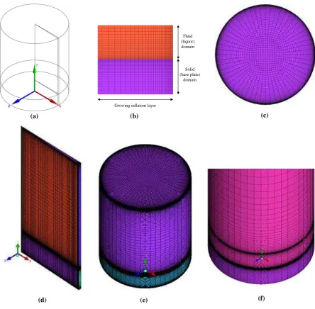
All of the geometries conform to a standard coordinate system as shown in Figure 6

(a). Hexahedral elements are used in all of the meshes for all of the geometries. Pertinent

flow features are well resolved such as near wall inflation as shown in Figure 6 (b). Near wall

inflation is used to ensure that the dimensionless wall distance, y+ ie less than 1 during the

simulations in order to capture the boundary layer resolution. This allows the full benefit of

the k - SST turbulence model to be harnessed since a low Reynolds number formulation

can be achieved inside the boundary layer. To minimise numerical diffusion, structured

meshes are generated, where the elements are positioned in the general direction of flow as

shown in Figure 6 (c - f). To minimise discretisation error the mesh quality, element

skewness and element orthogonally for every mesh is checked, and significant errors in the

mesh are rectified.

Mesh independence studies are conducted on all of the simulations presented in this

paper. The variables that are ensured to be mesh independent are the wall heat fluxes, wall

temperatures and fluid velocities at pertinent locations within the geometry. After mesh

independence studies the final mesh for the 2D axisymmetric case produces a mesh with

39330 elements (Figure 6 (d)). For the short test rig full 3D case, the final mesh after the

mesh sensitivity study produces a mesh with 422940 elements (Figure 6 (e)). Lastly, for the

tall test rig full 3D case, the final mesh after the mesh sensitivity study produces a mesh with

1205952 elements (Figure 6 (f)). These meshes are used to compute the final CFD solution.

The CFD simulations consist of three cases, (i) a 2D axisymmetric geometry for the

short test rig, (ii) a full 3D geometry for the short test rig, and (iii) a full 3D geometry for the

tall test rig. The Cartesian coordinate system defined in Figure 6 (a) is used as a reference to

present several plots of time averaged variables with respect to planar x or z directions, at

different vertical y positions. The time averaged results are presented after the initial transient

has dissipated sufficiently.

Figure 7 illustrates the time average velocity vectors superimposed onto time average

T* contours for the x – y plane for the short test rig. The size of the velocity vectors are

arbitrary and are used only to indicate circulation patterns occurring within the liquor. The

circulations of liquor are in disagreement between the 2D axisymmetric and the full 3D

geometries for the short test rig. In the 3D geometry liquor is driven vertically upwards at the

walls and returns vertically downward at the centreline. Conversely in the 2D axisymmetric

case the liquor is driven upward at the walls and the centre line (where the symmetry plane

occurs) and driven down the middle of the geometry. The simulations using a 2D

axisymmetric geometry produce an unphysical solution because the imposition of

axisymmetry enforces an unstable solution which is broken in the simulations using a full 3D

geometry. In the 2D axisymmetric case, the instantaneous time-dependent solution is forced

to be axisymmetric. In the full 3D case the instantaneous time-dependent fields are not

restricted to be axisymmetric. The time-averaged 3D solution is axisymmetric; however this

axisymmetric solution cannot be predicted using 2D axisymmetric conditions.

There is moderate agreement for the contours of time average T* in both 2D

axisymmetric and 3D cases. The time-averaged T* is more than 0 close to the upper plate

surface. This implies phase change is likely to occur close to the upper plate surface since the

Figure 8 is a plot of time average temperature and velocity for both 2D axisymmetric

and full 3D geometries for the short test rig, in the x – y plane. The effects of the unphysical

solution which the 2D axisymmetric simulation produces are seen. The 2D axisymmetric

geometry over predicts the values of temperature at the centreline (x = 0.00 m) and at the

walls (x = 0.05 m), and over predicts the values of velocity at the centreline (x = 0.00 m)

when compared to the equivalent 3D geometry.

Figure 9 is a plot of time average temperature and velocity for the full 3D geometry

for the short test rig, in the z – y plane. In this plot results from the 2D axisymmetric case are

absent since the 2D axisymmetric geometry exists only in the x – y plane. In Figure 9 the

values of time average temperatures and velocities in the z – y plane are largely the same as

the values of the time average temperatures and velocities in the x – y plane. This suggests the

full 3D short test rig does produce axisymmetric time-averaged results. Due to the unphysical

results which are produced using 2D axisymmetric conditions, only a full 3D simulation of

the tall test rig is performed.

Figure 10 illustrates the time average velocity vectors superimposed onto time

average T* contours for the x – y plane for the 3D tall test rig at the bottom, middle and top

sections of the test rig. The pattern of velocity circulations show the liquor is driven down the

walls and up the centre, which contrasts in behaviour for the 3D short test rig which does not

contain a draught tube. The presence of the draught tube in the tall test rig forces flow

reversal in the liquor. This suggests the draught tube has a large influence on the circulations

of the liquor. Since the draught tube in the tall test rig is implemented to represent the heating

coils of the Sellafield evaporators (see Figure 1), it can be hypothesised that the presence of

the coils in the Sellafield evaporators may have a similar effect on the liquor in the

evaporators. In Figure 10 at the lower test section the liquor is subcooled, where T* is less

0, and increases in value at the top of the test section at the free surface. The time average T*

contours suggest significant flashing from liquid to vapour may occur at the free surface,

since the pressure dependence of the saturation temperature is reduced here.

Figures 11 and 12 are plots of time average temperature and velocity in the x – y and

the x – z planes respectively. Symmetric conditions are largely found for the time average

temperature and velocity profiles for the tall test rig in the x – y and z – y planes respectively.

However in comparison to the short 3D case the free surface temperatures for the tall test rig

(at y = 2.225 m) vary significantly with position. Where as in the short case the free surface

temperature (at y = 0.12 m) remains largely symmetric.

Comparisons Between The Thermal Resistance and CFD Investigations

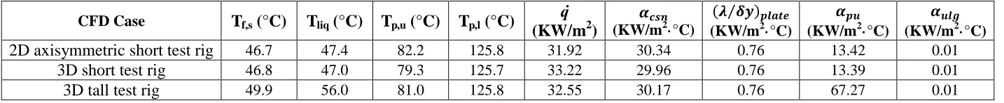
The area average temperatures, wall heat transfer coefficients and heat fluxes are

computed and are presented in Table 4 for the CFD investigations. There is poor agreement

between thermal resistance results for cases (a) and (b) in Tables 1 and 2 and the CFD results

in Table 4. The heat transfer coefficients produced by CFD at the upper plate are similar in

orders of magnitude to nucleate boiling. The results in Tables 1 and 2 from cases (a) and (b)

in the thermal resistance investigation do not predict nucleate boiling so have poor agreement

with the CFD results in Table 4. Table 3 for case (c) of the thermal resistance investigation

however provides reasonable agreement since the heat transfer coefficients used in case (c)

are for nucleate boiling which may occur as shown by the CFD results.

CONCLUSIONS

Thermal resistance networks are a computationally inexpensive tool to predict

temperatures, heat transfer coefficients and heat fluxes in a heat transfer system when

and free convection thermal resistance cases and the CFD investigation. There is however

reasonable agreement between the nucleate boiling case and CFD investigations. In the

nucleate boiling thermal resistance case there is good agreement between the six different

boiling heat transfer coefficients used, and the solutions in all three thermal resistance cases

are not sensitive to the type of condensation heat transfer coefficient used.

Poor flow physics is observed in the 2D axisymmetric geometry in the CFD

simulations of the short test rig because the symmetry planes enforce an unphysical solution

which is broken in the simulations using a full 3D geometry. Hence using 2D axisymmetric

conditions to model buoyancy driven flow in the test rigs is not prudent, even if the 3D

solution is symmetric. T* distributions in the short test rig indicate that nucleate boiling at the

upper plate may occur, and in the tall test rig the T* distributions indicate that the liquor is

heated above its saturation temperature in the upper regions of the test rig. The CFD

simulations have shown that phase change in the liquor is highly dependent on the pressure

head of the liquid column.

NOMENCLATURE

Specific heat capacity at constant pressure, J/kg·K

Constant depending on surface finish

Pressure correction factor

Gravitational acceleration, m/s2

Enthalpy of vaporisation, J/kg

Augmented enthalpy of vaporisation, J/kg

Characteristic length, m

Pressure, bar

Heat flux, W/m2

Thermal resistance, m2·°C/W

Roughness parameter, m

Temperature, °C

Time, s

Overall heat transfer coefficient, W/m2·K

Greek Symbols

Heat transfer coefficient, W/m2·°C

Expansion coefficient, °C-1

Vertical position, m

Horizontal position, m

Time step, s

A change in a property

Thermal conductivity, W/m·°C

Kinematic viscosity, m2/s

Viscosity, N·s/m2

Density, kg/m3 R

Surface tension, N/m

Gr Grashof number

Nu Nusselt number

Pr Prandtl number

Ra Rayleigh number

Dimensionless temperature

Subscripts

Reference

Boiling

Critical

Condensation

Convection

Free surface

Gas

Liquid

Liquor

Onset of nucleate boiling

Lower plate

Upper plate

Base plate

Reduced

Steam

Ullage

Wall

REFERENCES

[1] M. Wakem, T. Wylie, J. Spencer, G. Whillock, T. Ward, and S. Graham, “Heat

Transfer in a Highly Active Evaporator,” in 11th UK National Heat Transfer Conference, 2009.

[2] P. Upson, “Highly Active Liquid Waste Management at Sellafield,” Progress in Nuclear Energy, vol. 13, no. 1, pp. 31 – 47, 1984.

[3] W. Geddes, B. Perry, M. Wakem, and C. Wylie, “Boiling Heat Transfer in Highly

Active Liquors,” in 11th UK National Heat Transfer Conference, 2009.

[4] J. Thome, “Prediction of the Mixture Effect on Boiling in Vertical Thermosyphon Reboilers,” Heat Transfer Engineering, vol. 10, no. 2, pp 29 – 38, 1989.

[5] P. Heggs and C. Walton, “Precedence Ordering Techniques,” Institute of Mathematics and its Applications Conference Series, vol. 66, pp. 175 – 180, 1998.

[6] B. Perry and W. Geddes, “A Localised Condensation Model for the Simulation of

Kettle Evaporators,” in 12th UK National Heat Transfer Conference, 2011.

[7] W. Nusselt, “Die Oberflachenkondesation des Wasserdamffes,” Zetrschr. Ver. Deutch. Ing., vol. 60, pp. 541 – 546, 1916.

[8] A. Alane, “The Experimental Study of Operating Characteristics, Stability and

Performance of a Vertical Thermosyphon Reboiler Under Vacuum,” PhD Thesis, University of Manchester, 2007.

[9] J. Gerstmann and P. Griffith, “Laminar Film Condensation on the Underside of Horizontal and Inclined Surfaces,” International Journal of Heat and Mass Transfer, vol. 10, no. 5, pp. 567 – 570, 1967.

[10] W. Rohsenow, “Heat Transfer and Temperature Distribution in Laminar Film Condensation,” Trans. Asme, vol. 78, pp. 1645 – 1648, 1956.

[11] W. McAdams, Heat Transmission, 3rd Edition, McGraw-Hill, New York, 1954.

[12] P. Linstrom and W. Mallard, “NIST Chemistry Webbook; NIST Standard Reference

[13] H. Forster and N. Zuber, “Dynamics of Vapor Bubbles and Boiling Heat Transfer,” AIChE Journal, vol. 1, p. 531, 1955.

[14] I. Mostinski, “Application of the Rule of Corresponding States for Calculation of Heat Transfer and Critical Heat Flux,” Teploenergetika, vol. 4, pp. 66 – 71, 1963.

[15] K. Bier, J. Schmadl, and D. Gorenflo, “Influence of Heat Flux and Saturation Pressure on Pool Boiling Heat Transfer to Binary Mixtures.,” Chemical Engineering

Fundamentals, vol. 1, p. 79, 1983.

[16] M. Cooper, “Saturation Nucleate Pool Boiling: A Simple Correlation,” Chemical Engineering Symposium Series, vol. 86, p. 785, 1984.

[17] W. Rohsenow, “A Method of Correlating Heat Transfer Data for Surface Boiling of Liquids,” Trans. ASME, vol. 74, p. 969, 1951.

[18] G. Hewitt, G. Shires, and T. Bott, Process Heat Transfer. London: CRC Press, 1994.

[19] J. Collier and J. Thome, Convective Boiling and Condensation. Oxford University Press, 1996.

[20] W. Rohsenow, J. Hartnett, and Y. Cho, Handbook of Heat Transfer. New York: McGraw-Hill Book Company, 1998.

[21] F. Menter, “Two-equation Eddy-Viscosity Turbulence Models for Engineering Applications,” AIAA journal, 1994.

[22] S. Churchill and H. Chu, “Correlating Equations for Laminar and Turbulent Free Convection from a Vertical Plate,” International Journal of Heat and Mass Transfer, vol. 18, p. 1323, 1975.

Condensing

Correlation _(°C) (°C) (°C) (KW/m2) (KW/m2·°C) (KW/m2_·°C) (W/m2_·°C) (W/m2_·°C)

(W/m2·°C) (°C)

Case (a): Short Test Rig

Nusselt 102.5 126.7 126.9 0.15 181.91 0.76 6.13 2.62 1.83 0.48

Ger. and Gr. 102.5 126.7 126.9 0.15 41.77 0.76 6.13 2.62 1.83 0.48

Case (a): Tall Test Rig

Nusselt 56.9 126.8 126.9 0.02 358.53 0.76 0.28 1.74 0.24 0.10

Ger. and Gr. 56.9 126.8 126.9 0.02 67.97 0.76 0.28 1.74 0.24 0.10

Table 1: Results from case (a) of the thermal resistance investigation. Boundary conditions are steam and ullage temperatures, which have values

Condensing

correlation (°C) (°C) (°C) (°C) (KW/m2) (KW/m2_·°C) (KW/m2_·°C) (KW/m2_·°C) (KW/m2_·°C) (W/m2_·°C) (W/m2_·°C) (°C)

Case (b): Short Test Rig

Nusselt 125.7 126.1 126.6 126.9 0.23 157.67 0.76 0.52 0.52 2.85 2.81 0.59

Ger. and Gr. 125.7 126.1 126.5 126.8 0.23 37.69 0.76 0.52 0.52 2.85 2.81 0.59

Case (b): Tall Test Rig

Nusselt 125.7 126.1 126.6 126.9 0.23 157.67 0.76 0.52 0.52 2.85 2.81 0.36

Ger. and Gr. 125.7 126.1 126.5 126.8 0.23 37.69 0.76 0.52 0.52 2.85 2.81 0.36

Table 2: Results from case (b) of the thermal resistance investigation. Boundary conditions are steam and ullage temperatures, which have values

Boiling Correlation Condensing Correlation (°C) (°C)

(KW/m2) (KW/m2_·°C) (KW/m2_·°C) (KW/m2_·°C) (KW/m2_·°C) (°C)

Case (c): Short Test Rig

Forster and Zuber

Nusselt 60.96 125.02 48.36 26.45 0.76 3.64 0.61 8.65

Ger. and Gr. 60.74 122.44 46.58 10.56 0.76 3.56 0.59 8.49

Mostinskii Nusselt 59.96 124.98 49.10 26.32 0.76 3.99 0.62 8.72

Ger. and Gr. 59.82 122.36 47.22 10.52 0.76 3.89 0.60 8.55

Bier et al. Nusselt 56.42 124.85 51.67 25.87 0.76 5.90 0.65 8.94

Ger. and Gr. 56.31 122.08 49.65 10.40 0.76 5.74 0.63 8.77

Cooper Nusselt 48.10 124.54 57.71 24.94 0.76 132.00 0.73 9.45

Ger. and Gr. 48.10 121.39 55.34 10.13 0.76 128.34 0.70 9.25

Rohsenow Nusselt 55.65 124.82 52.23 25.78 0.76 6.54 0.66 8.99

Ger. and Gr. 55.55 122.01 50.18 10.37 0.76 6.37 0.63 8.81

Gorenflo and Kenning

Nusselt 64.44 125.15 45.84 26.92 0.76 2.73 0.58 8.42

Ger. and Gr. 64.31 122.73 44.11 10.70 0.76 2.65 0.56 8.26

Case (c): Tall Test Rig

Forster and Zuber

Nusselt 79.19 125.66 35.08 29.43 0.76 3.98 0.62 4.47

Ger. and Gr. 79.04 123.88 33.85 11.40 0.76 3.90 0.60 4.39

Mostinskii Nusselt 79.61 125.67 34.78 29.51 0.76 3.76 0.62 4.45

Ger. and Gr. 79.51 123.92 33.53 11.42 0.76 3.67 0.59 4.37

Bier et al. Nusselt 78.11 125.62 35.87 29.21 0.76 4.63 0.64 4.52

Ger. and Gr. 78.03 123.80 34.56 11.34 0.76 4.51 0.61 4.43

Cooper Nusselt 70.69 125.37 41.28 27.88 0.76 130.07 0.73 4.84

Ger. and Gr. 70.68 123.23 39.68 10.97 0.76 126.66 0.70 4.75

Rohsenow Nusselt 75.69 125.54 37.64 28.75 0.76 7.08 0.67 4.63

Ger. and Gr. 75.62 123.62 36.24 11.21 0.76 6.90 0.64 4.54

Gorenflo and Kenning

Nusselt 82.27 125.76 32.84 30.08 0.76 2.76 0.58 4.32

Ger. and Gr. 82.18 124.12 31.66 11.58 0.76 2.68 0.56 4.24

Table 3: Results from case (c) of the thermal resistance investigation. Boundary conditions are steam and liquor saturation temperatures, which

CFD Case Tf,s (°C) Tliq (°C) Tp,u (°C) Tp,l (°C) q

(KW/m2) (KW/m2_·°C) (KW/m2·°C) (KW/m

2

·°C) (KW/m

2

·°C)

2D axisymmetric short test rig 46.7 47.4 82.2 125.8 31.92 30.34 0.76 13.42 0.01

3D short test rig 46.8 47.0 79.3 125.7 33.22 29.96 0.76 13.39 0.01

3D tall test rig 49.9 56.0 81.0 125.8 32.55 30.17 0.76 67.27 0.01

List of Figure Captions

Figure 1: Arrangement of the Sellafield evaporators (not to scale), and the different heat

transfer regions.

Figure 2: Planar views of the (a) short test rig and (b) the tall test rig.

Figure 3: Thermal resistance networks for case (a) pure conduction through the liquor, case

(b) free convection in the liquor, and case (c) nucleate boiling in the liquor.

Figure 4: Temperature variations relative to the lower plate surface in the short test rig for the

pure conduction, free convection and nucleate boiling cases.

Figure 5: Temperature variations relative to the lower plate surface in the tall test rig for the

pure conduction, free convection and nucleate boiling cases.

Figure 6: (a) Cartesian coordinate system for the three geometries; (b) inflation layers in both

the solid (baseplate) and fluid (liquor) domains; (c) plan view of the structured hexahedral

mesh for the 3D short test rig; final mesh produced after mesh sensitivity studies for the (d)

2D axisymmetric short test rig; (e) 3D short test rig and (f) 3D tall test rig. Due to the height

of the tall test rig only the lower portion is pictured.

Figure 7: Contours of T* with superimposed velocity vectors showing the direction of

circulation in the x - y plane for the (left) 2D axisymmetric short test rig and (right) the 3D

short test rig.

Figure 8: Time average velocities and temperatures for the short test rig in the x – y plane.

Figure 10: Contours of T* with superimposed velocity vectors showing the direction of

circulation for the tall test rig in the x - y plane; from bottom (a) to top (g) in increments of

0.3164 m. The total height of the tall test rig is 2.215 m.

Figure 11: Transient average velocity and temperature for the tall test rig in the x plane.

Figure 1: Arrangement of the Sellafield evaporators (not to scale), and the different heat

transfer regions.

Region C

Region B

Region A Tsat(y)

0 Tstm

Tliq(y) Twall(y)

Figure 2: Planar views of the (a) short test rig and (b) the tall test rig. Condensing

Steam, Tstm Lower Plate Surface, Tpl Upper Plate Surface, Tpl

Liquor, Tliq Free Surface, Tfs

Ullage Space, Tulg

Condensing Steam, Tstm Lower Plate

Surface, Tpl Upper Plate Surface, Tpl Liquor, Tliq Free Surface, Tfs

Ullage Space, Tulg

Plate Height, yplate Liquor Depth, yliq Plate Height, yplate Liquor Depth, yliq

Figure 3: Thermal resistance networks for case (a) pure conduction through the liquor, case

(b) free convection in the liquor, and case (c) nucleate boiling in the liquor.

q



q



q



q



Tstm 126.85 °C Tpu Tpl R1 R2 Tsat

Short rig 51.71 °C Tall rig 70.37 °C

R3

Flashing Tulg

45.8 °C

q



q



Figure 4: Temperature variations relative to the lower plate surface in the short test rig for the

pure conduction, free convection and nucleate boiling cases.

0.00 0.05 0.10 0.15

40 50 60 70 80 90 100 110 120 130

0.00 0.05 0.10 0.15

40 50 60 70 80 90 100 110 120 130

Heigh

t F

ro

m Lo

wer Plate Su

rfac

e (m)

Temperature Using Nu. Condensing Coefficient (°C)

Pure Conduction Free Convection Forster and Zuber Mostinskii Bier et al. Cooper Rohsenow

Gorenflo and Kenning

Temperature Using Ger. and Gr. Condensing Coefficient (°C)

Heigh

t F

ro

m Lo

wer Plate Su

rfac

e (m)

Pure Conduction Free Convection Forster and Zuber Mostinskii Bier et al. Cooper Rohsenow

Figure 5: Temperature variations relative to the lower plate surface in the tall test rig for the

pure conduction, free convection and nucleate boiling cases.

0.0 0.5 1.0 1.5 2.0 2.5

50 60 70 80 90 100 110 120 130

0.0 0.5 1.0 1.5 2.0 2.5

50 60 70 80 90 100 110 120 130

Temperature Using Nu. Condensing Coefficient (°C)

Height From

Lower Pl

ate Surface (m)

Pure Conduction Free Convection Forster and Zuber Mostinskii

Bier et al. Cooper Rohsenow

Gorenflo and Kenning

Temperature Using Ger. and Gr. Condensing Coefficient (°C)

Height From

Lower Pl

ate Surface (m)

Pure Conduction Free Convection Forster and Zuber Mostinskii

Bier et al. Cooper Rohsenow

Fluid (liquor) domain

Solid (base plate)

domain

Growing inflation layer

(a) (b) (c)

(d) (e) (f)

Figure 6: (a) Cartesian coordinate system for the three geometries; (b) inflation layers in both

the solid (baseplate) and fluid (liquor) domains; (c) plan view of the structured hexahedral

mesh for the 3D short test rig; final mesh produced after mesh sensitivity studies for the (d)

2D axisymmetric short test rig; (e) 3D short test rig and (f) 3D tall test rig. Due to the height

Figure 7: Contours of T* with superimposed velocity vectors showing the direction of

circulation in the x - y plane for the (left) 2D axisymmetric short test rig and (right) the 3D

Figure 8: Time average velocities and temperatures for the short test rig in the x – y plane. 45 50 55 60 65 70

-0.06 -0.04 -0.02 0.00 0.02 0.04 0.06

-0.06 -0.04 -0.02 0.00 0.02 0.04 0.06

0.00 0.01 0.02 0.03 0.04

T

rn

.

A

v

g

.

T

emp

er

at

u

re

(

ºC

)

2D AS y = 0.03 m 2D AS y = 0.07 m 2D AS y = 0.12 m 3D y = 0.03 m 3D y = 0.07 m 3D y = 0.12 m

T

rn

.

A

v

g

.

V

el

o

ci

ty

(

m/s

)

Figure 9: Time average velocities and temperatures for the short test rig in the z – y plane. 45

50 55 60

-0.06 -0.04 -0.02 0.00 0.02 0.04 0.06

-0.06 -0.04 -0.02 0.00 0.02 0.04 0.06

0.00 0.01 0.02 0.03

T

rn

.

A

v

g

.

T

emp

er

at

u

re

(

°C)

3D y = 0.03 m 3D y = 0.07 m 3D y = 0.12 m

T

rn

.

A

v

g

.

V

el

o

ci

ty

(

m/s

)

(a) (b) _(c)

(d) (e) (f) (g)

Figure 10: Contours of T* with superimposed velocity vectors showing the direction of

circulation for the tall test rig in the x - y plane; from bottom (a) to top (g) in increments of

Figure 11: Transient average velocity and temperature for the tall test rig in the x plane. 48 50 52 54 56 58 60 62

-0.06 -0.04 -0.02 0.00 0.02 0.04 0.06

-0.06 -0.04 -0.02 0.00 0.02 0.04 0.06

0.00 0.02 0.04 0.06 0.08 0.10 0.12

T

rn

.

A

v

g

.

T

emp

er

at

u

re

(

ºC

)

3D y = 0.03 m 3D y = 1.1275 m 3D y = 2.225 m

T

rn

.

A

v

g

.

V

el

o

ci

ty

(

m/s

)

Figure 12: Transient average velocity and temperature for the tall test rig in the z plane. 46 47 48 49 50 51 52 53 54 55 56 57 58 59 60 61

-0.06 -0.04 -0.02 0.00 0.02 0.04 0.06

-0.06 -0.04 -0.02 0.00 0.02 0.04 0.06

0.00 0.02 0.04 0.06 0.08 0.10 0.12

T

rn

.

A

v

g

.

T

emp

er

at

u

re

(

ºC

)

3D y = 0.03 m 3D y = 1.1275 m 3D y = 2.225 m

T

rn

.

A

v

g

.

V

el

o

ci

ty

(

m/s

)

45

Jujar S. Panesar is a PhD doctoral researcher in the Energy, Technology and

Innovation Initiative (ETII) group at the University of Leeds, UK. He is

currently investigating heat transfer and multiphase flows occurring within

low pressure evaporators which are used in the British nuclear reprocessing

industry. Before beginning his PhD he received a BEng(hons) degree in Mechanical

Engineering from Queen Mary, University of London, and an MSc in Computational Fluid

Dynamics from University of Leeds, and previously worked as a graduate design engineer at

Sizewell B nuclear power station.

Peter Heggs, FREng, FIChemE, CEng, CSci, BSc, PhD (Leeds) is an Emeritus

Professor of the University of Manchester, and currently, is a Visiting Research

Professor in SPEME at the University of Leeds. He spent 4 years in the USA

with Union Carbide Corporation and then became an academic at the

Universities of Leeds, Bradford, UMIST and Manchester. He is currently the Chairman of

the Heat Transfer Steering Panel of ESDU International, a member of the UK Heat Transfer

Committee and a past President of the UK Heat Transfer Society. He has supervised 63

Masters and 56 PhD students, published over 300 research papers and has contributed to 34

books or parts of books. His research interests include the design, control and operability of

46

Dr Alan D. Burns is a senior developer of the commercial CFD code Ansys

CFX, and an honorium senior lecturer in the Energy, Technology and

Innovation Initiative (ETII) group at the University of Leeds, UK. His research

interests are in numerical algorithms, mathematical models and applications of multiphase

flows. He obtained an MA(hons) in Mathematics from Trinity College, Cambridge, and a

PhD in Mathematical Physics from the University of Durham.

Lin Ma, PhD (Leeds) is Senior Lecturer at the Energy Technology and

Innovation Initiative (ETII) and CFD Centre, Faculty of Engineering of the

University of Leeds. He has supervised 14 PhD students, published over 150

research papers and has contributed to 6 book chapters. His research interests include wind

energy, coal/biomass combustion for power generation, and carbon capture and sequestration

technologies.

Dr Stephen J. Graham is a Laboratory Fellow at the National Nuclear

Laboratory. He has 25 years’ experience in the application of CFD in the

nuclear industry. He is an active peer reviewer and chairs two working groups

associated with technical quality in modelling and simulation. His current

research interests include the application of CFD to multiphase flows. After obtaining a

BSc(hons) in physics at the University of Sheffield, he gained a PhD for his work in