White Rose Research Online URL for this paper:
http://eprints.whiterose.ac.uk/90956/
Version: Accepted Version
Article:
Aram, P., Kadirkamanathan, V. and Anderson, S.R. (2015) Spatiotemporal System
Identification With Continuous Spatial Maps and Sparse Estimation. IEEE Transactions on
Neural Networks and Learning Systems, 26 (11). pp. 2978-2983. ISSN 2162-237X
https://doi.org/10.1109/TNNLS.2015.2392563
[email protected] https://eprints.whiterose.ac.uk/
Reuse
Unless indicated otherwise, fulltext items are protected by copyright with all rights reserved. The copyright exception in section 29 of the Copyright, Designs and Patents Act 1988 allows the making of a single copy solely for the purpose of non-commercial research or private study within the limits of fair dealing. The publisher or other rights-holder may allow further reproduction and re-use of this version - refer to the White Rose Research Online record for this item. Where records identify the publisher as the copyright holder, users can verify any specific terms of use on the publisher’s website.
Takedown
If you consider content in White Rose Research Online to be in breach of UK law, please notify us by
Spatiotemporal System Identification with
Continuous-spatial-maps and Sparse Estimation
Parham Aram*, Visakan Kadirkamanathan
Member, IEEE
and Sean R. Anderson
Abstract—In this paper we present a framework for the identification for spatiotemporal linear dynamical systems. We use a state-space model representation, which has the following attributes: the number of spatial observation locations are decoupled from the model order; the model allows for spatial heterogeneity; the model representation is continuous-over-space; the model parameters can be identified in a simple, sparse estimation procedure. The model identification procedure we propose has four steps: (i) decomposition of the continuous spatial field using a finite set of basis functions. Spatial fre-quency analysis is used to determine basis function width and spacing such that the main spatial frequency contents of the underlying field can be captured; (ii) initialisation of states in closed form; (iii) initialisation of state-transition and input matrix model parameters using sparse regression - the least absolute shrinkage and selection operator (lasso) method; (iv) joint state and parameter estimation using an iterative Kalman-filter/sparse-regression algorithm. To investigate the performance of the proposed algorithm we use data generated by the Kuramoto model of spatiotemporal cortical dynamics. The identification algorithm performs successfully, predicting the spatiotemporal field with high accuracy, whilst the sparse regression leads to a compact model.
Index Terms—spatiotemporal, system identification, space-time modelling, sparse regression
I. INTRODUCTION
S
PATIOTEMPORAL systems modelling is becoming an important area of study in such diverse areas as meteorol-ogy [1], biomedical signal processing [2], the neurosciences [3], epidemiology [4], and mobile sensor networks [5]. In order to fully describe the underlying dynamics of such processes, it is generally recognised that space and time data should not be treated as statistically independent variables [6]. Recent advances in data collection techniques and computing power have made possible the development of unifying methods of spatial interpolation and temporal prediction. This paper intro-duces an efficient data-driven method to build a sparse model of linear spatiotemporal systems with continuous-spatial-maps. To identify spatiotemporal models of linear dynamical sys-tems the space-time, auto-regressive, moving average, with exogenous input (STARMAX) model was developed as a specialist form of multivariate ARMAX model [7], [8]. There are two important limitations of the STARMAX model, how-ever: (i) the number of observation locations is intrinsically coupled to the order of the model, hence model size grows with the number of observation locations and (ii) the modelP. Aram, V. Kadirkamanathan and S. R. Anderson are with the Department of Automatic Control and Systems Engineering, University of Sheffield, Mappin Street, Sheffield, S1 3JD, UK. (email: [email protected]). P. Aram is also with the Insigneo Institute for in silico Medicine, Sheffield, S1 3JD, UK.
describes behaviour at discrete spatial locations only and therefore cannot produce continuous-spatial maps. The former is a particular disadvantage for system identification, where compact models for systems-level analysis is often a key goal. Additionally, there are many circumstances where a continuous-spatial map would be preferable to predictions at discrete spatial locations.
An innovation pursued by a number of researchers centred around an approach where the spatiotemporal model was described in a state-space form and the continuous spatial field was represented by a basis function decomposition [9]– [11]. The weights of the basis functions themselves were then described as a dynamic process, evolving over time in the state vector. This approach had the dual advantages over STARMAX of describing the spatial field as a continuous map, as well as decoupling the model order from the number of observation locations. However, the dynamics tended to be defined in terms of a simple process such as a random walk [9], or derived froma prioriknowledge of the physical process [12]. These approaches opened up a key gap: the use of data-driven techniques to identify the dynamics of the spatiotemporal system, which was addressed recently us-ing system identification techniques for the integro-difference equation (IDE) model representation [13], [14].
However, the IDE model discussed in [13], [14] has a disadvantage in that the spatial mixing kernel used to describe correlations over space assumes homogeneity: all points in space are described by the same mixing kernel - an assumption that may be limiting in some circumstances. One advantage of the STARMAX model, in this regard, is that it allows for heterogeneity in the spatial correlations, whilst being amenable to data-driven identification. Therefore, this leads us to the conclusion that the three broad approaches to spatiotemporal modelling described above (STARMAX, basis function de-composition of the spatial field and data-driven identification) have attributes that have not yet been distilled into a single, powerful framework for system identification that incorporates the following: (i) decoupled number of sensor observations from model order; (ii) continuity-in-space; (iii) a heterogenous representation; (iv) data-driven methods for the identification of process dynamics. Deriving such a framework is the aim of this paper.
output equation of a state-space model; in the second step the states are initialised in closed form from the spatial observation data; in the third step the model parameters are initialised using either a least squares (LS) technique or a sparse regression technique - least absolute shrinkage and selection operator (lasso) [15]–[17]. The key advantage of using lasso is that it simultaneously identifies spatial correlation structure along with estimating model parameters. In the fourth step the states and parameters are estimated in a joint procedure using an iterative Kalman-filter/sparse-regression algorithm, inspired by a similar LS approach [18].
The structure of the paper is as follows. In Section II a finite dimensional state-space representation of the dynamic spatial field is derived where the continuous spatial field is approximated using a basis function decomposition. Section III provides conditions based on spatial frequency analysis to determine both basis function width and spacing such that, the main spatial frequency contents of the underlying field can be captured. The joint estimation method for state and sparse parameter estimation is described in Section IV. Finally the main results of the paper are summarised in Section V.
II. SPATIOTEMPORAL MODELLING
The aim of this section is to derive a finite dimensional state-space representation of the dynamic spatial field. The output equation is a basis function representation of the spatial field and the state equation describes the dynamic evolution of the basis function weights, where the weights themselves are modelled as a space-time autoregressive with exogenous input (ARX) process. The resulting model represents spatio-temporal processes as a continuous spatial field with discrete temporal dynamics.
A. Continuous spatial field representation
The continuous spatial field is observed at spatial position
s∈Rns (where n
s≤3) and discrete timet is given by
yt(sny) =
Z
Ω
m(sny−s′)zt(s′)ds′+ǫt(sny), (1)
wherezt(s)is the continuous spatial field,m(·)is the sensor
kernel and ǫt ∼ N(0,Σǫ)is an independent and identically
distributed (i.i.d.) Gaussian white noise process with the covariance matrix Σǫ =σǫ2Iny, whereI denotes the identity
matrix. Using an appropriate set of basis functions that spans the function space in which the spatial field is defined, zt(s)
can be decomposed as
zt(s) = ∞
X
i=1
xi,tφi(s), (2)
where xi,t are the dynamic coefficients of the expansion at
time t, and φi(s) are static basis functions. Truncating the
sum in equation (2) at i=nxleads to an approximate
repre-sentation with a finite number of basis functions, weighted by a finite dimensional state vector, xtof dimensionnx, i.e.,
zt(s)≈φ⊤(s)xt. (3)
The field basis functions used here aren-dimensional Gaussian functions given by
φ(s) = exp −(s−µφ)
⊤(s−µ φ)
σ2 φ
!
. (4)
where σφ and µφ are the basis function width and centre
respectively. The widths of the basis functions as well as the placement of basis functions can be chosen by spectral analysis (see Section III). Substituting equation (3) back into equation (1) we have
yt(sny) =
Z
Ω
m(sny−s
′)φ⊤(s′)ds′x
t+ǫt(sny). (5)
In a matrix form (5) can be re-written as
yt=Cxt+ǫt, (6)
where yt =
yt(s1) yt(s2) . . . yt(sny)
⊤
and ǫt =
ǫt(s1) ǫt(s2) . . . ǫt(sny)
⊤
. Each element of the obser-vation matrix,C, is given by
Cij=
Z
Ω
m(si−s′)φj(s′) ds′. (7)
When point sensors are used equation (7) simplifies to
Cij =φj(si). (8)
B. Dynamic evolution of the spatial field
In order to link the dynamic coefficients over time we assume an evolution equationf(·)such that
xt+1=f(xt,ut,et), (9)
whereutis the input at timetandetaccounts for unmodelled
terms and approximated by a zero mean Gaussian disturbance with the covariance matrix,Σe. Assumingf(·)is a linear time
invariant map, equation (9) can be written in a form of
xt+1=Axt+But+et. (10)
where A∈ Rnx×nx, B ∈Rnx×nu. This completes the final
form of the state-space model.
The state-space representation is based on the basis de-composition of the spatial field where the accuracy (degree of smoothness) of the model can be determined by spatial frequency analysis (explained in detail in the following sec-tion). The spectral low-pass action of these basis functions can attenuate the high spatial frequency variations in the observed field. Therefore, care must be taken to ensure that any estimation procedure applied to the observed field adequately captures the high spatial frequency variations by adjustment of the basis function hyperparameters.
III. SPATIAL FREQUENCY ANALYSIS
still be found if the spatial field is only approximately band limited, i.e.
Zt(ν)≈0 ∀ν>νcy, (11)
where Zt(ν) is the spatial Fourier transform of zt(s), ν is
the spatial frequency and νcy is the cutoff frequency of the
observed field. For an approximate reconstruction of such a band-limited field, the distance between centres of adjacent basis functions, ∆φ, must be
∆φ ≤ 1 2ρνcy
, (12)
where ρ ∈ R ≥ 1 is an oversampling parameter [14]. This is analogous to the Nyquist criterion in temporal frequency domain.
In case of Gaussian basis functions, for a 3 dB attenuation atνcy the width can be obtained by [21]
σ2φ= ln 2 2π2
1
ν⊤ cyνcy
. (13)
The number of basis functions can be determined by dividing spatial field of interest into∆φintervals. The complexity of the
state-space model (number of basis functions) can be reduced by choosing wider basis functions. This will indeed result into a less accurate (smoother) estimation. In this case the cut-off frequency of the estimated field,νcφ, can be set into a desired
value by tuning the width of the basis functions , i.e.,
νcφ= 1
πσφ
r
ln 2
2 . (14)
In this case, the reconstructed field can represent the spatial frequency contents of the observed field upto νcφ. The
dis-tance, ∆φ, can be also determined by substitutingνcφforνcy
in equation (12), i.e.,
∆φ≤ 1 2ρνcφ
. (15)
From reciprocal role of νcφ in equation (15) it follows that
for a more detailed representation of the spatial field a higher number of basis functions is required. This, in turn, leads to increase in number of states in the state-space represen-tation. Therefore, a compromise should be made between the accuracy and the computational demands of the estimation algorithm.
IV. SPATIOTEMPORAL MODEL PARAMETER ESTIMATION
In this section, we describe the estimation procedure for the state-space model. An iterative state-parameter estimation algorithm with lasso is derived for sparse modelling, with simple initialisation steps.
A. Joint sparse parameter and state estimation
Spatiotemporal systems can often incur many parameters in their description. For instance, naive estimation of the space model defined here would lead to a full state-transition matrix, implicitly assuming non-zero spatial cor-relations amongst all basis functions. Alternatively, we can usually obtain a model with far fewer parameters using sparse
regression methods. Here, we use lasso to obtain a sparse model of the system dynamics, which simultaneously identifies spatial correlation along with model parameters.
A complication arises because the states and parameters of the state-space model are both unknown and therefore require joint estimation. One well-known method for joint state-parameter estimation is to augment the state vector with the model parameters and solve the resulting nonlinear filtering problem via the extended Kalman filter (EKF) [22] or Rao-Blackwellised particle filter (RBPF) [23]. A robust joint state-parameter estimation algorithm could be used to improve the convergence and the accuracy of the EKF algorithm [24] but this algorithm does not give a sparse solution for the param-eters. For the particle filter, the nature of the spatiotemporal problem renders the state dimension too high for computing efficiently by current RBPF algorithms.
A solution, therefore, to this problem is to use an itera-tive two-stage state-parameter estimation algorithm: a step of Kalman filtering (or smoothing) to estimate the state sequence, followed by a step of parameter estimation by LS [3], [18]. We extend this algorithm here to a sparse version where we use lasso in the parameter estimation step.
The task is to estimate both states and parameters from a set ofT data-samples,
( ˆΘ,x1:ˆ T) = arg min Θ,x1:T
J(Θ,x1:T), (16)
where
Θ = θ⊤1, . . . ,θ⊤nx
⊤
(17)
θi= (ai,1, . . . , ai,nx, b1,1, . . . , bi,nu) ⊤
, i= 1, . . . , nx
(18)
where individual parameter vectorsθi pertain to the dynamic
evolution of each separate basis function, where aij and bij
are theijth elements of the transition matrix,A, and the input matrix,B. The joint state-parameter cost functionJ(Θ,x1:T)
is defined as
J(Θ,x1:T) = T
X
t=1
xt+1−A(Θ)xt−B(Θ)ut
2 2,
+ T
X
t=1
yt−Cxt
2 2+λ
Θ
1 (19)
where the system matrices are written as functions of Θ to indicate their dependence on the model parameters. Then for the case of a known state sequence the joint cost function reduces to
J(θi|x1:T) =
zi−Xθi
2 2+λ
θi
1, i= 1, . . . , nx (20)
whereλ≥0is a regularisation weighting parameter (note the cost function reduces to the LS problem treated in [18] for
λ= 0), and where
where
zi= (xi,t+1, . . . , xi,t+T)⊤, (22)
xi,t+1= (x1,t, . . . , xnx,t, u1,t, . . . , unu,t)θi+ei,t, (23)
ei= (ei,t, . . . , ei,t+T)⊤, (24)
and
X=
x1,t . . . xn
x,t u1,t . . . unu,t x1,t+1 . . . xn
x,t+1 u1,t+1 . . . unu,t+1 ..
. ... ... ... ...
x1,t+T
−1 . . . xnx,t+T−1 u1,t+T−1 . . . unu,t+T−1
.
(25)
The solution to the lasso problem defined in (20) cannot be expressed in a closed-form but there exists many efficient algorithms to compute the solution [25]. Here we use a cyclical coordinate descent algorithm computed along a path of values of the regularisation parameter λ [26]. Efficient implementations of this algorithm are available in the Matlab statistics toolbox (the lasso function) and the Python scikit-learn module [27]. The regularisation parameter λ can either be chosen by user inspection because the path algorithm intrinsically generates results for a sequence ofλvalues, orλ
can be chosen by cross-validation.
For known parameters, the joint cost function J(Θ,x1:T)
reduces to
J(x1:T|Θ) = T
X
t=1
xt+1−Axt−But
2 2+
T
X
t=1
yt−Cxt
2 2
(26) which can be solved for the estimated state-sequence x1:ˆ T
using the Kalman smoother (or the Kalman filter for greater computational efficiency) [28].
The joint cost function J(Θ,x1:T) can be solved
sequen-tially by iterative minimisation of J(θi|x1:T)andJ(x1:T|Θ)
[18]. The complete estimation framework for spatiotemporal system identification is given in Algorithm 1 with initialisation steps for the states discussed below.
The iterative estimation of states and parameters in step 4 of Algorithm 1 can be viewed as coordinate descent in the variablesx1:T andΘ, and forλ= 0is guaranteed convergent
to a local optimum of the cost function J(Θ,x1:T) [18],
subject to the following conditions: (i) that the state-space model is observable and unique - satisfied here due to the canonical form imposed by the representation of the spatial field basis function decomposition in the state-space model and (ii) that the input is persistently exciting, which is satisfied by the definition of the state noise signal et.
For λ > 0, convergence of the joint sparse parameter-state estimation problem is dependent on convergence of the lasso algorithm. This is usually not an issue in practice for the fast path descent algorithm used here, but we note that if guaranteed convergence is required then the lasso problem is also equivalent to minimising the sum-of-squared residual errors,zi−Xθi
2
2, subject to the constraint|θi|1≤γ, where
γ is a threshold parameter. For this constrained optimisation problem, the cost function is convex, and the constraints define
a convex set. Hence, the lasso solution can be found by using standard quadratic programming methods for guaranteed convergence.
Therefore, as each step of state and parameter estimation in Algorithm 1 is guaranteed to converge, the joint cost function J(Θ,x1:T) is guaranteed to be non-increasing, i.e.
Jk(Θ,x1:T) ≤ Jk−1(Θ,x1:T) ≤ . . . ≤ J1(Θ,x1:T), where
the subscriptkindicates algorithm iterations. The convergence of the parameters can be monitored using a measure such as the change in the Frobenius norm, k · kF, of the parameters Θacross iterations and the algorithm can be set to stop when k · kF crosses some threshold.
B. State initialisation
The state vector comprises the basis function weights of the spatial field decomposition. State estimation at each time-step is therefore a straightforward task, given a defined set of basis functions in the observation matrixC, where
ˆ
xt=C†yt, t= 1. . . T (27)
Note that the pseudo inverse, C† = C⊤C−1
C⊤, for state
[image:5.612.343.534.342.484.2]estimation only needs to be calculated once.
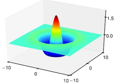
Fig. 1. Finite width spatial kernel corresponding to the fourth derivative of a Gaussian. The spatial kernel governs the couplings between oscillators.
V. SIMULATION AND RESULTS
A. Data generation
To investigate the performance of the proposed algorithm we use data generated using Kuramoto model of coupled phase oscillators [29]. The Kuramoto model has been successfully used to explicate synchronisation in a range of biological and physical phenomena [30]. In [31] the spatial aspect of neuronal connectivity is introduced to the Kuramoto model to exhibit dynamics similar to cortical activities. The Kuramoto model in this formulation is given by a set of N spatially coupled differential equations:
˙
θn=ωn+
K N
N
X
m=1
W(m, n) sin (θm−θn), (28)
where θn denotes the phase of oscillator n with the natural
frequencyωn,K is the coupling constant andW(m, n)is a
−10
0 10
Space
(a) (b) (c)
(d) (e) (f)
(g) (h) (i) 0
32 64
0 32 64
0 32 64
−10
0 10
Space
0 32 64
0 32 64
0 32 64
0 10
Space
−10
0 10
Space
0 32 64
−10 0 10
Space
0 32 64
−10 0 10
Space
[image:6.612.99.523.53.397.2]0 32 64
Fig. 2. Examples of actual and estimated spatial fields for three time instants. The first column shows the actual spatial fields. The second and third columns show the estimated spatial fields using LS and lasso method respectively.
Algorithm 1. Spatiotemporal system identification. 1. Spatial field decomposition:
-define basis function widthsσφ using (13),
-define basis function centres µφ ,
-construct observation matrix elements Cij using (7).
2. State initialisation:
-constructC†= C⊤C−1 C⊤,
-estimate state sequence x1:ˆ T using (27),
3. Parameter initialisation:
-constructX0 fromx1:ˆ T using (25),
-estimate parametersΘ0ˆ usingX0 and (20),
4. Joint state and parameter estimation: -define stopping condition thresholdρ, -setk= 1,
while ||Θk−Θk−1||F > ρ
-parameterise the state-space model by Θˆk−1,
-update the state sequencex1:ˆ T by
minimisation of (26) and hence redefineXk,
-update the parameters Θˆk usingXk and (20),
-setk=k+ 1,
end while
coupling between nodesmandn. We used the code provided by [31] to generate2s of data sampled at 1 kHz with a60×60
grid of oscillators. All other parameters selected to be the same as used in [31]. The spatial kernel is shown in Fig. 1 which is the fourth derivative of a Gaussian function. Examples of the simulated spatial field are plotted in the first column of Fig. 2 which shows traveling wave-like patterns in the system. The spatial field was observed using a30×30regular lattice of point sensors and measurements were corrupted by a zero mean Gaussian white noise with Σǫ= 0.2×Iny.
B. Spatiotemporal system identification
The spatiotemporal system identification algorithm defined in Algorithm 1 was used here to identify the Kuramoto model. The observation noise covariance was known to the estimator and the disturbance covariance was set toΣe= 0.1×I. The
spatial frequency analysis was used to specify the arrangement of basis functions. The lasso regularisation parameter λwas tuned to 0.1 using the rapid parameter initialisation method, and this value was subsequently used in the full joint state-parameter estimation algorithm.
The cutoff frequency of the observed spatial field is
0.26cycles/mm. Substituting this for νcy in (12) with ρ= 2
yielded a minimum spacing of 0.96, giving an equal grid of
full spatial frequency contents from observations. We limited the spatial contents of the estimated field in favour of a simpler model with smaller number of basis functions. Setting
σ2
φ = 2.5 into (14) resulted into νcφ = 0.12. Given the
limited cutoff frequency and the over sampling parameter an equal grid of 12×12 basis functions were used to construct the state-space model. This results into a less accurate and smoother estimation, however, has the advantage of reducing the computational complexity of the estimation algorithm.
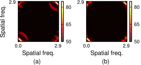
The results of the spatial field estimation for three time instants are illustrated in Fig. 2, showing a good estimation accuracy for both LS and lasso based algorithm. The effect of using a lower cutoff frequency, νcφ, in the reconstructed
field can be seen in Fig. 3, reducing the spatial bandwidth of the approximated field compared to the observed one. In
0.0 2.9
Spatial freq.
2.9
S
p
a
ti
a
l
fr
e
q
.
(a) (b)
50 65 80
0.0 2.9
Spatial freq.
2.9
[image:7.612.62.292.249.356.2]50 65 80
Fig. 3. Spatial frequency analysis. (a) The average (over time) power in dB of the spatial field. (b) The average (over time) power in dB of the reconstructed field.
order to compare the two methods we calculated the root mean square error (RMSE) over space of the field estimation for each time instant. The result is shown in Fig. 4(a), showing a slightly better performance where LS algorithm was used. The accuracy of the estimates was also evaluated by comparing the field reconstruction to the true field using the mean (over time) of the variance account for (MVAF) over space, giving 81.4% and 80.5% for LS and lasso based algorithm respectively. The rates of convergence of the two methods are depicted in Fig. 4(b), showing a slower rate for the LS based algorithm. Here we used the absolute change in the Frobenius norms of the successive estimates of A matrices as the stopping criterion.
Although the performance of the LS based algorithm is slightly better than its lasso based counterpart, the lasso based algorithm results in far fewer model parameters as demon-strated in Fig. 5. In fact only 43.2% of the elements in the transition matrix, A, are non-zero. The comparison between the two methods is summarised in Table. I. The results demonstrate a trade-off between accuracy and sparsity but the encouraging feature is that over half the model parameters can be set to zero with a only a∼1% drop in prediction accuracy (i.e. for λ= 0.1).
VI. SUMMARY
In this paper we have developed a novel method for spa-tiotemporal system identification for linear dynamical systems. The identification framework has the following attributes: (i)
Comparison of LS and lasso based algorithms, and different values of regularisation parameterλ.
Method λvalue MVAF % of non-zero elements inAˆ
LS 0 81.4% 100% lasso 0.01 81.4% 97% lasso 0.1 80.5% 43.2% lasso 0.3 77.1% 26.8% lasso 1 56.2% 12.5%
0 1 2
Time (sec)
5 15 25
RMSE
(a) (b)
1 10 20
Iteration
0.0 0.1
F
rob
enius
no
rm
Fig. 4. (a) Error in the field reconstruction. The RMSE of the estimated field over time for LS and lasso method. (b) Plot of the absolute change in Frobenius norms ofAˆfor successive iterations of the algorithm. In each subplot the LS and lasso based algorithm are shown by solid and dashed lines respectively.
1 72 144
72 144
(a) (b)
−0.1
0.0 0.1
1 72 144
72 144
Fig. 5. Parameter estimation. (a) The result of sparse parameter estimation using lasso. (b) The binary representation of the transition matrix estimate,
ˆ
A, using lasso method. The nonzero elements ofAˆis replaced by ones for a better visualisation.
the number of spatial observation locations are decoupled from the model order; (ii) the dynamics of the system are identified by sparse regression (lasso), resulting in a compact model; (iii) the model allows for spatial heterogeneity; (iv) the model rep-resentation is continuous-over-space. We have demonstrated by a numerical example that the proposed method can produce compact models of complex spatiotemporal systems.
VII. ACKNOWLEDGMENT
Prof Kadirkamanathan acknowledges the support of the EPSRC (EP/H00453X/1).
REFERENCES
[1] C. K. Wikle, R. Madden, and T. Chen, “Seasonal variation of upper tropospheric and lower stratospheric equatorial waves over the tropical Pacific,”Journal of the Atmospheric Sciences, vol. 54, no. 14, pp. 1895– 1909, 1997.
[image:7.612.329.545.345.436.2][3] P. Aram, D. Freestone, M. Dewar, K. Scerri, V. Jirsa, D. Grayden, and V. Kadirkamanathan, “Spatiotemporal multi-resolution approximation of the Amari type neural field model,”NeuroImage, vol. 66, pp. 88–102, 2012.
[4] L. A. Waller, B. P. Carlin, H. Xia, and A. E. Gelfand, “Hierarchical spatio-temporal mapping of disease rates,” Journal of the American Statistical Association, vol. 92, no. 438, pp. 607–617, 1997.
[5] D. Gu and H. Hu, “Spatial Gaussian process regression with mobile sensor networks,”IEEE Trans. Neural Networks and Learning Systems, vol. 23, pp. 1279–1290, Aug. 2012.
[6] N. Cressie and C. K. Wikle, Statistics for Spatio-Temporal Data. Hoboken, New Jersey: Wiley, 2011.
[7] P. E. Pfeifer and S. J. Deutsch, “Independence and sphericity tests for the residuals of space-time arma models,”Communications in Statistics - Simulation and Computation, vol. 9, no. 5, pp. 533–549, 1980. [8] D. S. Stoffer, “Estimation and identification of space-time ARMAX
models in the presence of missing data,” Journal of the American Statistical Association, vol. 81, no. 395, pp. 762–772, 1986.
[9] J. R. Stroud, P. Muller, and B. Sanso, “Dynamic models for spatiotem-poral data,”Journal of the Royal Statistical Society. Series B, vol. 63, no. 4, pp. 673–689, 2001.
[10] C. K. Wikle, “A kernel-based spectral approach for spatio-temporal dynamic models,” inProceedings of the 1st Spanish Workshop on Spatio-Temporal Modelling of Environmental Processes (METMA), Benicassim, Spain , Oct. 2001, pp. 167–180.
[11] ——, “A kernel-based spectral model for non-Gaussian spatio-temporal processes,”Statistical Modelling, vol. 2, no. 4, pp. 299–314, 2002. [12] ——, “Hierarchical Bayesian models for predicting the spread of
eco-logical processes,”Ecology, vol. 84, no. 6, pp. 1382–1394, 2003. [13] M. Dewar, K. Scerri, and V. Kadirkamanathan, “Data-driven
spatio-temporal modeling using the integro-difference equation,”IEEE Trans. Signal Processing, vol. 57, pp. 83–91, Jan. 2009.
[14] K. Scerri, M. Dewar, and V. Kadirkamanathan, “Estimation and model selection for an IDE-based spatio-temporal model,”IEEE Trans. Signal Processing, vol. 57, pp. 482–492, Feb. 2009.
[15] R. Tibshirani, “Regression shrinkage and selection via the lasso,”
Journal of the Royal Statistical Society. Series B (Methodological), pp. 267–288, 1996.
[16] V. Roth, “The generalized LASSO,” IEEE Trans. Neural Networks, vol. 15, pp. 16–28, Jan. 2004.
[17] B. Efron, T. Hastie, I. Johnstone, and R. Tibshirani, “Least angle regression,”The Annals of Statistics, vol. 32, no. 2, pp. 407–499, 2004. [18] M. Chadwick, S. R. Anderson, and V. Kadirkamanathan, “An iterative Kalman smoother/least-squares algorithm for the identification of delta-ARX models,”International Journal of Systems Science, vol. 41, no. 7, pp. 839–851, 2010.
[19] R. Sanner and J. Slotine, “Gaussian networks for direct adaptive control,”
IEEE Trans. Neural Networks, vol. 3, pp. 837–863, Nov. 1992. [20] D. Peterson and D. Middleton, “Sampling and reconstruction of
wave-number-limited functions in n-dimensional Euclidean spaces,” Informa-tion and Control, vol. 5, pp. 279–323, 1962.
[21] D. R. Freestone, P. Aram, M. Dewar, K. Scerri, D. B. Grayden, and V. Kadirkamanathan, “A data-driven framework for neural field modeling,”NeuroImage, vol. 56, no. 3, pp. 1043–1058, 2011. [22] L. Ljung and T. Soderstrom,Theory and Practice of Recursive
Identifi-cation. Cambridge, MA: The MIT Press, 1983.
[23] P. Li, R. Goodall, and V. Kadirkamanathan, “Estimation of parameters in a linear state space model using a Rao-Blackwellised particle filter,”
IEE Proceedings-Control Theory and Applications, vol. 151, no. 6, pp. 727–738, 2004.
[24] J. Xiong and T. Zhou, “Parameter identification for nonlinear state-space models of a biological network via linearization and robust state estimation,” in Proceeding of the 32nd Chinese Control Conference. IEEE, Xian, China, Jul. 2013, pp. 8235–8240.
[25] T. Hastie, R. Tibshirani, and J. Friedman, The Elements of Statistical Learning: Data Mining, Inference and Prediction, 2nd ed. New York: Springer, 2009.
[26] J. Friedman, R. Tibshirani, and T. Hastie, “Regularization paths for generalized linear models via coordinate descent,”Journal of Statistical Software, vol. 33, no. 1, 2010.
[27] F. Pedregosa, G. Varoquaux, A. Gramfort, V. Michel, B. Thirion, O. Grisel, M. Blondel, P. Prettenhofer, R. Weiss, V. Dubourget al., “Scikit-learn: Machine learning in python,” The Journal of Machine Learning Research, vol. 12, pp. 2825–2830, 2011.
[28] T. Kailath, A. H. Sayed, and B. Hassibi, Linear Estimation. Upper Saddle River, NJ: Prentice Hall, 2000.
[29] Y. Kuramoto,Chemical Oscillations, Waves, and Turbulence. Mineola, New York: Dover Publications, 2003.
[30] J. Acebr´on, L. Bonilla, C. Vicente, F. Ritort, and R. Spigler, “The Kuramoto model: A simple paradigm for synchronization phenomena,”
Reviews of Modern Physics, vol. 77, no. 1, p. 137, 2005.