Compressive Sensing Approaches for Autonomous Object Detection in Video Sequences

This is a repository copy of

Compressive Sensing Approaches for Autonomous Object

Detection in Video Sequences

.

White Rose Research Online URL for this paper:

http://eprints.whiterose.ac.uk/92123/

Version: Accepted Version

Proceedings Paper:

Kuzin, D., Isupova, O. and Mihaylova, L. (2015) Compressive Sensing Approaches for

Autonomous Object Detection in Video Sequences. In: Sensor Data Fusion: Trends,

Solutions, Applications (SDF), 2015. Sensor Data Fusion: Trends, Solutions, Applications

(SDF), 2015, 6-8 Oct. 2015, Bonn, Germany. IEEE .

https://doi.org/10.1109/SDF.2015.7347706

[email protected] https://eprints.whiterose.ac.uk/

Reuse

Unless indicated otherwise, fulltext items are protected by copyright with all rights reserved. The copyright exception in section 29 of the Copyright, Designs and Patents Act 1988 allows the making of a single copy solely for the purpose of non-commercial research or private study within the limits of fair dealing. The publisher or other rights-holder may allow further reproduction and re-use of this version - refer to the White Rose Research Online record for this item. Where records identify the publisher as the copyright holder, users can verify any specific terms of use on the publisher’s website.

Takedown

If you consider content in White Rose Research Online to be in breach of UK law, please notify us by

Compressive Sensing Approaches for Autonomous

Object Detection in Video Sequences

Danil Kuzin

Sheffield, UK

Email: [email protected]

Olga Isupova

Sheffield, UK

Email: [email protected]

Lyudmila Mihaylova

Sheffield, UK

Email: [email protected]

Abstract—Video analytics requires operating with large amounts of data. Compressive sensing allows to reduce the number of measurements required to represent the video using the prior knowledge of sparsity of the original signal, but it imposes certain conditions on the design matrix. The Bayesian compressive sensing approach relaxes the limitations of the conventional approach using the probabilistic reasoning and allows to include different prior knowledge about the signal structure. This paper presents two Bayesian compressive sensing methods for autonomous object detection in a video sequence from a static camera. Their performance is compared on real datasets with the non-Bayesian greedy algorithm. It is shown that the Bayesian methods can provide more effective results than the greedy algorithm in terms of both accuracy and computational time.

I. INTRODUCTION

The significant developments in the field of sparse meth-ods during the last decades lead to the new research and application fields. One of the first applications of sparse modelling is the linear regression problem where l0 and l1

-norm regularisation is considered. The latter has the advantage that a norm term is convex, while it has not so obvious sparse interpretation [1].

Sparse modelling is further developed in the field of signal processing in compressive sensing [2], where the main idea is to extract only the meaningful information from the mea-surements. Two main problems are considered in compressive sensing: selecting the optimal design matrix and solving ill-posed regression, that arises in the original signal decoding from the measurements [3].

In Bayesian modelling sparseness of the data can be achieved by imposing special sparse prior distributions [4]. For example, in [5] the authors propose the Laplace prior on the data. The full inference to this model is provided in [6], using the Expectation Propagation (EP) technique. Another work is [7], where the prior is modified to the hierarchical Gaussian-Gamma distribution. These models are used as a basis for Bayesian compressive sensing in [8] and [9].

The overview of recently developed sparse algorithms and models for image and video processing is presented in [10]. One of the essential problems in video process-ing is autonomous object detection which is mostly solved by background subtraction. Background subtraction aims to distinguish the foreground (moving objects) from the

back-ground (static ones). Sparseness is natural for the backback-ground subtraction problem as the foreground objects occupy the small regions on a frame. Background subtraction hence represents a natural application area for sparse modelling.

The idea to apply compressive sensing for background subtraction is proposed, for example, in [11] and developed in [12]. In contrast to these works in this paper we focus on the sparse Bayesian methods for background subtraction and the comprehensive comparison of these methods with the conventional compressive sensing one.

The contribution of this paper is the development of a Bayesian compressive sensing algorithm for the background subtraction problem. In Bayesian compressive sensing the estimated sparse coefficients are random variables with some prior distribution. Also this paper presents the comparison of several algorithms to evaluate their applicability in different situations.

This paper is organised as follows. In Section II the pro-posed approach is described. The experimental results are presented in Section III. Section IV concludes the paper and discusses the future work.

II. FRAMEWORK

Assume that we have a static camera. The frame B ∈

Rn1×n2 _{at a time instant} 0 _{is considered as a background} frame. The video from the camera consists of the sequential framesVk ∈Rn1×n2, k ∈ {1, . . . , K}. The aim is to detect the moving objects in these frames.

A. Video preprocessing

The camera provides video frames in the Red-Green-Blue (RGB) format and they are next converted to the greyscale format. For the purposes of the compressive sensing approach the frames are converted to vectors. Thus, the background frame B is converted to a vector b∈ Rn_{, the video frames}

Vk are converted to vectorsvk ∈Rn, where n=n1n2. B. Compressive sensing

The non-zero elements of the difference fk = vk −b are supposed to correspond to the moving objects. As the foreground objects take only a part of the image the vector

fk has many values that are close to zero:

l0-pseudonorm is the number of non-zero elements of a vector.

Within the compressive sensing approach the number of measurements that are need to be taken can be reduced [2] and the image quality may be improved [10]. The values of the vectorfk are calculated based on the set of the compressed measurements gk∈Rs:

gk=Φfk, (2)

where the design matrixΦ∈Rs×n consists of i.i.d Gaussian variables. It is selected according to the method proposed in [13].

Since fk =vk−b, the computation of the coefficients gk can be done on the acquisition step as

gk =Φfk =Φvk−Φb. (3) The vectors Φb and Φvk are linear combinations of the pixels of the video frames. Therefore, a single pixel camera may be used. It means that the acquisition and background subtraction steps use the signal with the lengthsrather thann. The reconstruction step is used to restore the signal with the length n.

The linear system (3) is underdetermined when n > sand therefore an infinite number of solutions exists. The problem can be determined by introducing a sparse structure in the

fk signal. This can be done by lp norm minimisation, where p <2 typically.

The sparse methods for this kind of problems are [14, Chapter 13]:

• l₀ - minimisation. The greedy algorithms based on least

squares estimates, stochastic search, variational inference;

• l₁ - minimisation. The coordinate descent, LARS, the

proximal and gradient projection methods;

• Non-convex minimisation. The bridge regression, the

hi-erarchical adaptive lasso.

In this paper we focus on the Bayesian compressive sensing methods [8], [15] and compare them with orthogonal match-ing pursuit (OMP) [16], that is a greedy algorithm for l0

-minimisation.

1) Bayesian compressive sensing (BCS): The system (3) is

reformulated as a linear regression model in [8]:

gk=Φfk+ξ, (4)

whereξis a vector which elements are the independent noise from the Gaussian distribution:ξi∼ N(ξi; 0, β−1

). Therefore, the likelihood can be expressed as

p(gk|fk, β) = n

Y

i=1

N(gi,k;Φifk, β

−1

), (5)

wheregi,k is thei-th element of the vectorgk,Φi – thei-th row of the matrix Φ.

To implement the full Bayesian approach, the prior distri-butions are imposed on all the parameters:

p(fk|α) = n

Y

i=1

N(fi,k; 0, α−i1), (6)

where fi,k is the i-th element of the vector fk, α is a prior parameter vector,αi is the i-th element of the vectorα;

p(α) = n

Y

i=1

Γ(αi;a, b), (7)

p(β) = Γ(β;c, d), (8)

whereΓ(·)denotes the Gamma distribution. The values of the hyperparametersa, b, c, dare set uniform and close to zero.

According to the Bayes rule the posterior distribution can be written as follows:

p(fk,α, β|gk) =

p(gk|fk,α, β)p(fk,α, β) p(gk)

, (9)

wherep(gk|fk,α, β)is the likelihood term, p(fk,α, β)is the prior term, p(gk) is the evidence term. The latter can be expressed as:

p(gk) =

Z

fk,α,β

p(gk|fk,α, β)p(fk,α, β)dfkdαdβ. (10)

This integral is intractable, therefore some kind of approxima-tion should be used.

In Bayesian compressive sensing [8] the decomposition of the posterior probability into the product of the tractable and intractable probabilities is used and the intractable one is approximated with the delta-function in its mode:

p(fk,α, β|gk) =p(fk|gk,α, β)p(α, β|gk). (11) The Bayes rule for the first term of (11) is as follows:

p(fk|gk,α, β) =

p(gk|fk, β)p(fk|α) p(gk|α, β)

. (12)

These are all the Gaussians, so the probabilityp(fk|α, β,gk) can be calculated straightforwardly. It is the Gaussian distri-bution with the parameters

Σ= (βΦ⊤Φ+A)−1

, (13)

µ=βΣΦ⊤gk, (14)

whereA=diag(α1, . . . , αn).

The second term of the posterior probability (11) can be expressed as:

p(α, β|gk) =

p(gk|α, β)p(α)p(β) p(gk)

. (15)

The denominator in (15) is not tractable. The values ofα, β which maximise (15) are used. The hyperpriors are uniform, therefore only the termp(gk|α, β)needs to be maximised:

p(gk|α, β) =

Z

p(gk|fk, β)p(fk|α)dfk. (16) Maximisation of (16) w.r.t. α, β gives the following iterative process:

αnewi = γi µ2

i

, (17)

(β−1)new₌ kgk−Φµk

2

l2

(a) (b) (c) (d) (e)

(f) (g) (h) (i) (j)

(k) (l) (m) (n) (o)

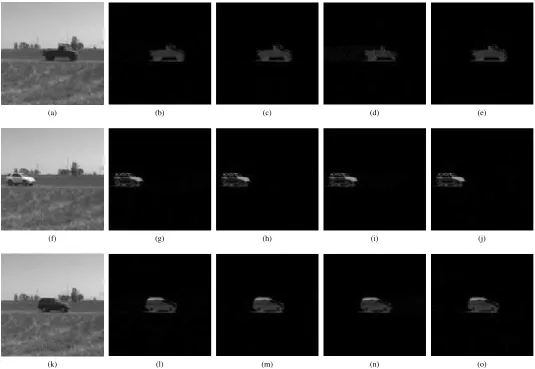
Figure 1. Comparison of the foreground restoration based on 2000 measurements by the algorithms. The three rows correspond to the three sample frames. From left to right columns: the input uncompressed frame, uncompressed background subtraction, compressed background subtraction with Bayesian compressive sensing, compressed background subtraction with multi-task Bayesian compressive sensing and compressed background subtraction with orthogonal matching pursuit

whereγi= 1−αiΣii.

This process together with (13) – (14) converges to the optimal estimates.

Note that

p(fi,k) =b a_Γ

a+1 2

(2π)12Γ(a)

b+f

2

i,k 2

!−(a+12)

. (19)

This is the Student-t distribution that has the most probable area concentrated around zero. Thereby it leads to the sparse vector fk.

2) Multitask Bayesian compressive sensing (Multitask

BCS): In [15] the Bayesian method to process several signals

that have a similar sparse structure is proposed. The multitask setting reduces the number of measurements that should be taken compared to processing all the signals independently. The hyperparameter α is considered to be shared by all the tasks.

3) Matching Pursuit: The greedy algorithms are proposed

for the l0 minimisation in [16]. These methods start with a

null vector and iteratively add non-zeros values to it until a convergence to a threshold.

III. EXPERIMENTS

We use the Convoy dataset [12], which consists of 260 greyscale frames and the background frame. The frames are scaled to the less resolution of 128×128 to avoid memory problems. For the multitask algorithm the batches of 40 frames are run together, while for the Bayesian compressive sensing and OMP algorithms all the frames are processed independently. There are two sets of the experiments: one with s = 2000 measurements and the other with s = 5000 measurements. For both sets of the experiments all three meth-ods are run for 10 times with 10 different design matricesΦ

shared among the methods. For the quantitative comparison the median values of quality measures among these runs are presented.

(a) (b) (c) (d) (e)

(f) (g) (h) (i) (j)

(k) (l) (m) (n) (o)

Figure 2. Comparison of the foreground restoration based on 5000 measurements by the algorithms. The three rows correspond to the three sample frames. From left to right columns: the input uncompressed frame, uncompressed background subtraction, compressed background subtraction with Bayesian compressive sensing, compressed background subtraction with multi-task Bayesian compressive sensing and compressed background subtraction with orthogonal matching pursuit

demonstrative frames are presented. One can notice that with the same design matrix the models demonstrate similar results. The figures show that 2000 measurements can be used for object region detection, while 5000 measurements which is only about 30% of the input resolution are enough even to distinguish parts of the objects like doors and windows of the cars.

For the quantitative comparison of the results the following measures are used:

• Reconstruction error: kf −

ˆ_fkl 2

kfkl2

, where f is the signal

ground truth, ˆf is the signal, reconstructed by the algo-rithm;

• Background subtraction quality measure (BS quality):

|S(f)∩S(ˆf)|

|S(f)∪S(ˆf)|,whereS(f)is the ground truth foreground

area,S(ˆf)is the algorithm detected foreground area,| · |

is the cardinality of the set;

• Peak signal-to-noise ratio (PSNR):

10 log10

peakval2 MSE

, where peakval is the maximum

possible pixel value, that is 255 in our case. MSE is the mean square error betweenf andˆf;

• Structural similarity index (SSIM) [17]:

(2µ_fµˆ_f +C1)(2σ_fˆ_f +C2)

(µ2

f +µ

2

ˆ_f +C1)(σ2

f +σ

2 ˆ

f +C2)

, where µ_f, µˆ_f, σ_f,

σˆ_f, σ_fˆ_f are the local means, standard deviations, and

cross-covariance for the images f, ˆf respectively, and C1, C2 are the regularisation constants.

The difference between the uncompressed current frame vk and the uncompressed background frame b is used as the ground truth signal f for every frame (the second columns in Figures 1 – 2), since this is the signal which is compressed by (3).

50 100 150 200 250 0.4

0.6 0.8 1

Frames

Error

Reconstruction error

(a)

50 100 150 200 250

0.2 0.4 0.6 0.8

Frames

Error

Reconstruction error

(b)

50 100 150 200 250

0 0.2 0.4 0.6 0.8 1

Frames

Quality

BS quality

(c)

50 100 150 200 250

0 0.2 0.4 0.6 0.8 1

Frames

Quality

BS quality

(d)

50 100 150 200 250

30 40 50 Frames PSNR PSNR measure (e)

50 100 150 200 250

35 40 45 50 55 Frames PSNR PSNR measure (f)

50 100 150 200 250

0.5 0.6 0.7 0.8 0.9 1

Frames

SSIM

SSIM measure

(g)

50 100 150 200 250

0.85 0.9 0.95 1

Frames

SSIM

SSIM measure

(h)

, xshift=0.5ex, yshift=0.5exOMP , xshift=0.5ex, yshift=0.5exBCS , xshift=0.5ex, yshift=0.5exMT-BCS

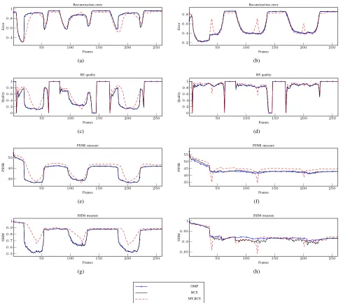
Figure 3. Quantitative method comparison on the frame level. The left column corresponds to the set of the experiments with 2000 measurements, the right column corresponds to the set of the experiments with 5000 measurements. From top to bottom rows: the reconstruction error measure (values close to 1 refer to the frames without any foreground objects), the background subtraction quality measure, the PSNR measure and the SSIM measure.

Table I

METHOD COMPARISON BASED ON2000MEASUREMENTS.

Algorithm Mean frame recon-struction error Mean frame BS quality Mean frame PSNR Mean frame SSIM Mean compu-tational time (hours)1

BCS 0.8037 0.3518 34.2007 0.7198 0.23

Multitask BCS

0.7608 0.4820 37.542 0.8384 0.67

OMP 0.8028 0.3510 34.1705 0.7204 0.51

1_{The computational time is provided for a batch of 40 frames (BCS and}

OMP process each frame independently with 4 parallel workers, multitask BCS processes all 40 frames together). Implementation is made on the laptop with i7-4702HQ CPU with 2.20GHz, 16 GB RAM using MATLAB 2015a.

Table II

METHOD COMPARISON BASED ON5000MEASUREMENTS.

Algorithm Mean frame recon-struction error Mean frame BS quality Mean frame PSNR Mean frame SSIM Mean compu-tational time (hours)1

BCS 0.4713 0.8119 43.8251 0.9186 0.9

Multitask BCS

0.4702 0.8421 45.0028 0.9212 8.5

OMP 0.4578 0.8109 43.2720 0.9266 4.8

mea-sure. The Bayesian compressive sensing and OMP algorithms show the competitive results but the Bayesian compressive sensing algorithm works faster. It is worth while to note that the multitask Bayesian compressive sensing algorithm has the biggest variance amongst the runs with the different design matrices, while the variances of the Bayesian compressive sensing and OMP runs for the same matrices are quite small.

IV. CONCLUSIONS AND FUTURE WORK

This work presents two Bayesian compressive sensing al-gorithms for autonomous object detection in video sequences. These are the conventional Bayesian compressive sensing and the multitask Bayesian compressive sensing algorithms. The results presented in Figures 1 – 2 demonstrate the appropriate reconstruction quality of the original image based on only 5000 measurements (that is≈30% of the original image size). The conventional Bayesian compressive sensing method demonstrates similar results to the greedy OMP algorithm but the former is more effective in terms of the computational time. If the computational time is not critical the extension of the Bayesian method designed for a multitask problem can improve the performance in terms of the different measures. Therefore, other extensions of the Bayesian method to include the prior information need further research.

Future work will be focused on different sparse Bayesian methods, such as the EP-based framework with the Laplace prior proposed in [6] and the Markov Chain Monte Carlo (MCMC) framework proposed in [18]. Future work will also consider a correlated sparse structure of the data.

V. ACKNOWLEDGEMENTS

The authors Olga Isupova and Lyudmila Mihaylova are grateful for the support provided by the EC Seventh Frame-work Programme [FP7 2013-2017] TRAcking in compleX sensor systems (TRAX) Grant agreement no.: 607400. Lyud-mila Mihaylova acknowledges also the support from the UK Engineering and Physical Sciences Research Council (EPSRC) via the Bayesian Tracking and Reasoning over Time (BTaRoT) grant EP/K021516/1.

REFERENCES

[1] F. Bach, R. Jenatton, J. Mairal, and G. Obozinski, “Optimization with sparsity-inducing penalties,”Found. Trends Mach. Learn., vol. 4, no. 1, pp. 1–106, Jan. 2012.

[2] E. Candes and M. Wakin, “An introduction to compressive sampling,” IEEE Signal Processing Magazine, vol. 25, no. 2, pp. 21–30, March 2008.

[3] A. Y. Carmi, L. S. Mihaylova, and S. J. Godsill, “Introduction to com-pressed sensing and sparse filtering,” inCompressed Sensing and Sparse Filtering, ser. Signals and Communication Technology, A. Y. Carmi, L. Mihaylova, and S. J. Godsill, Eds. Springer Berlin Heidelberg, 2014, pp. 1–23.

[4] N. G. Polson and J. G. Scott, “Shrink globally, act locally: Sparse Bayesian regularization and prediction,”Bayesian Statistics, vol. 9, pp. 501–538, 2010.

[5] R. Tibshirani, “Regression shrinkage and selection via the lasso,” Jour-nal of the Royal Statistical Society. Series B (Methodological), vol. 58, no. 1, pp. 267–288, 1996.

[6] M. Seeger, “Bayesian inference and optimal design in the sparse linear model,”Journal of Machine Learning Research, vol. 9, pp. 759–813, 2008.

[7] M. E. Tipping, “Sparse Bayesian learning and the relevance vector machine,”The journal of machine learning research, vol. 1, pp. 211– 244, 2001.

[8] S. Ji, Y. Xue, and L. Carin, “Bayesian compressive sensing,” IEEE Transactions on Signal Processing, vol. 56, no. 6, pp. 2346–2356, June 2008.

[9] M. W. Seeger and H. Nickisch, “Compressed sensing and Bayesian ex-perimental design,” inProceedings of the 25th International Conference on Machine Learning, ser. ICML ’08. New York, NY, USA: ACM, 2008, pp. 912–919.

[10] J. Mairal, F. R. Bach, and J. Ponce, “Sparse modeling for image and vision processing,”CoRR, vol. abs/1411.3230, 2014.

[11] V. Cevher, A. Sankaranarayanan, M. F. Duarte, D. Reddy, and R. G. Baraniuk, “Compressive sensing for background subtraction,” in Euro-pean Conf. Comp. Vision (ECCV), 2008, pp. 155–168.

[12] G. Warnell, S. Bhattacharya, R. Chellappa, and T. Basar, “Adaptive-rate compressive sensing using side information,”ArXiv e-prints, Jan. 2014. [13] R. Baraniuk, M. Davenport, R. DeVore, and M. Wakin, “A simple proof of the restricted isometry property for random matrices,”Constructive Approximation, vol. 28, no. 3, pp. 253–263, 2008.

[14] K. P. Murphy,Machine Learning: A Probabilistic Perspective. The MIT Press, 2012.

[15] S. Ji, D. Dunson, and L. Carin, “Multitask compressive sensing,”IEEE Transactions on Signal Processing, vol. 57, no. 1, pp. 92–106, Jan 2009. [16] S. Mallat and Z. Zhang, “Matching pursuits with time-frequency dictio-naries,”IEEE Transactions on Signal Processing, vol. 41, no. 12, pp. 3397–3415, Dec 1993.

[17] Z. Wang, A. Bovik, H. Sheikh, and E. Simoncelli, “Image quality assess-ment: from error visibility to structural similarity,”IEEE Transactions on Image Processing, vol. 13, no. 4, pp. 600–612, April 2004. [18] T. Park and G. Casella, “The Bayesian lasso,”Journal of the American