DOI 10.1007/s10107-014-0814-9
F U L L L E N G T H PA P E R
Decomposition algorithms for submodular optimization
with applications to parallel machine scheduling
with controllable processing times
Akiyoshi Shioura · Natalia V. Shakhlevich · Vitaly A. Strusevich
Received: 7 May 2013 / Accepted: 1 September 2014 / Published online: 17 September 2014 © The Author(s) 2014. This article is published with open access at Springerlink.com
Abstract In this paper we present a decomposition algorithm for maximizing a linear function over a submodular polyhedron intersected with a box. Apart from this con-tribution to submodular optimization, our results extend the toolkit available in deter-ministic machine scheduling with controllable processing times. We demonstrate how this method can be applied to developing fast algorithms for minimizing total com-pression cost for preemptive schedules on parallel machines with respect to given release dates and a common deadline. Obtained scheduling algorithms are faster and easier to justify than those previously known in the scheduling literature.
Keywords Submodular optimization·Parallel machine scheduling· Controllable processing times·Decomposition
Mathematics Subject Classification 90C27·90B35·90C05
Supported by the EPSRC funded project EP/J019755/1 and partially by the Humboldt Research Fellowship of the Alexander von Humboldt Foundation and by Grant-in-Aid of the Ministry of Education, Culture, Sports, Science and Technology of Japan.
A. Shioura
Graduate School of Information Sciences, Tohoku University, Sendai, Japan e-mail: [email protected]
N. V. Shakhlevich
School of Computing, University of Leeds, Leeds LS2 9JT, UK e-mail: [email protected]
V. A. Strusevich (
B
)1 Introduction
In scheduling with controllable processing times, the actual durations of the jobs are not fixed in advance, but have to be chosen from a given interval. This area of scheduling has been active since the 1980s, see surveys [16] and [22].
Normally, for a scheduling model with controllable processing times two types of decisions are required: (1) each job has to be assigned its actual processing time, and (2) a schedule has to be found that provides a required level of quality. There is a penalty for assigning shorter actual processing times, since the reduction in processing time is usually associated with an additional effort, e.g., allocation of additional resources or improving processing conditions. The quality of the resulting schedule is measured with respect to the cost of assigning the actual processing times that guarantee a certain scheduling performance.
As established in [23,24], there is a close link between scheduling with controllable processing times and linear programming problems with submodular constraints. This allows us to use the achievements of submodular optimization [4,21] for design and justification of scheduling algorithms. On the other hand, formulation of scheduling problems in terms of submodular optimization leads to the necessity of studying novel models with submodular constraints. Our papers [25,27] can be viewed as convincing examples of such a positive mutual influence of scheduling and submodular optimiza-tion.
This paper, which builds up on [26], makes another contribution towards the devel-opment of solution procedures for problems of submodular optimization and their applications to scheduling models. We present a decomposition algorithm for maxi-mizing a linear function over a submodular polyhedron intersected with a box. Apart from this contribution to submodular optimization, our results extend the toolkit avail-able in deterministic machine scheduling. We demonstrate how this method can be applied to several scheduling problems, in which it is required to minimize the total penalty for choosing actual processing times, also known as total compression cost. The jobs have to be processed with preemption on several parallel machines, so that no job is processed after a common deadline. The jobs may have different release dates.
The paper is organized as follows. Section2gives a survey of the relevant results on scheduling with controllable processing times. In Sect. 3 we reformulate three scheduling problems in terms of linear programming problems over a submodular polyhedron intersected with a box. Section4outlines a recursive decomposition algo-rithm for solving maximization linear programming problems with submodular con-straints. The applications of the developed decomposition algorithm to scheduling with controllable processing times are presented in Sect.5. The concluding remarks are contained in Sect.6.
2 Scheduling with controllable processing times: a review
cost for schedules that are feasible with respect to given release dates and a common deadline.
Formally, in the model under consideration the jobs of setN = {1,2, . . . ,n}have to be processed on parallel machinesM1,M2, . . . ,Mm, wherem ≥ 2. For each job
j ∈ N, its processing time p(j)is not given in advance but has to be chosen by the decision-maker from a given interval
p(j),p(j)
. That selection process can be seen as eithercompressing(also known ascrashing) the longest processing timep(j)down top(j), ordecompressingthe shortest processing timep(j)up top(j). In the former case, the valuex(j)= p(j)−p(j)is called thecompression amountof job j, while in the latter casez(j)= p(j)−p(j)is called thedecompression amountof job j. Compression may decrease the completion time of each job j but incurs additional costw(j)x(j), wherew(j)is a given non-negative unit compression cost. The total cost associated with a choice of the actual processing times is represented by the linear functionW =j∈Nw(j)x(j).
Each job j ∈ Nis given arelease date r(j), before which it is not available, and a commondeadline d, by which its processing must be completed. In the processing of any job,preemptionis allowed, so that the processing can be interrupted on any machine at any time and resumed later, possibly on another machine. It is not allowed to process a job on more than one machine at a time, and a machine processes at most one job at a time.
Given a schedule, letC(j)denote the completion time of job j, i.e., the time at which the last portion of job j is finished on the corresponding machine. A schedule is calledfeasible if the processing of a job j ∈ N takes place in the time interval [r(j),d].
We distinguish between theidentical parallel machines and theuniformparallel machines. In the former case, the machines have the same speed, so that for a job j with an actual processing time p(j)the total length of the time intervals in which this job is processed in a feasible schedule is equal to p(j). If the machines are uniform, then it is assumed that machineMhhas speedsh,1≤h ≤m. Without loss
of generality, throughout this paper we assume that the machines are numbered in non-increasing order of their speeds, i.e.,
s1≥s2≥ · · · ≥sm. (1)
For some schedule, denote the total time during which a jobj ∈ Nis processed on machineMh,1≤h ≤m, byqh(j). Taking into account the speed of the machine, we
call the quantityshqh(j)theprocessing amountof job j on machineMh. It follows
that
p(j)=
m
h=1
shqh(j).
problems of this type byα|r(j),p(j)= p(j)−x(j),C(j)≤d,pmt n|W. Here, in the first fieldαwe write “P” in the case ofm ≥ 2 identical machines and “Q” in the case ofm ≥ 2 uniform machines. In the middle field, the item “r(j)” implies that the jobs have individual release dates; this parameter is omitted if the release dates are equal. We write “p(j) = p(j)−x(j)” to indicate that the processing times are controllable andx(j)is the compression amount to be found. The condition “C(j)≤d” reflects the fact that in a feasible schedule the common deadline should be respected. The abbreviation “pmt n” is used to point out that preemption is allowed. Finally, in the third field we write the objective function to be minimized, which is the total compression costW =j∈Nw(j)x(j). Scheduling problems with control-lable processing times have received considerable attention since the 1980s, see, e.g., surveys by Nowicki and Zdrzałka [16] and by Shabtay and Steiner [22].
If the processing times p(j), j ∈ N, are fixed then the corresponding coun-terpart of problem α|r(j),p(j) = p(j)−x(j),C(j) ≤ d,pmt n|W is denoted by α|r(j),pmt n|Cmax. In the latter problem it is required to find a preemptive
schedule that for the corresponding settings minimizes the makespan Cmax =
max{C(j)|j ∈N}.
In the scheduling literature, there are several interpretations and formulations of scheduling models that are related to those with controllable processing times. Below we give a short overview of them, indicating the points of distinction and similarity with our definition of the model.
Janiak and Kovalyov [8] argue that the processing times areresource-dependent, so that the more units of a single additional resource is given to a job, the more it can be compressed. In their model, a job j ∈ N has a ‘normal’ processing time b(j)(no resource given), and its actual processing time becomes p(j) = b(j)− a(j)u(j), provided thatu(j)units of the resource are allocated to the job, wherea(j) is interpreted as a compression rate. The amount of the resource to be allocated to a job is limited by 0≤ u(j)≤ τ(j), whereτ(j)is a known job-dependent upper bound. The cost of using one unit of the resource for compressing jobjis denoted byv(j), and it is required to minimize the total cost of resource consumption. This interpretation of the controllable processing times is essentially equivalent to that adopted in this paper, which can be seen by setting
p(j)=b(j), p(j)=b(j)−a(j)τ(j), x(j)=a(j)u(j), w(j)=v(j)/a(j), j ∈ N.
A very similar model for scheduling with controllable processing times is due to Chen [2], later studied by McCormick [13]. For example, McCormick [13] gives algorithms for finding a preemptive schedule for parallel machines that is feasible with respect to arbitrary release dates and deadlines. The actual processing time of a job is determined byp(j)=max{b(j)−a(j)λ(j),0}and the objective is to minimize the functionj∈Nλ(j). This is also similar to our interpretation due to
Another range of scheduling models relevant to our study belongs to the area of imprecise computation; see [12] for a recent review. In computing systems that support imprecise computation, some computations (image processing programs, implemen-tations of heuristic algorithms) can be run partially, producing less precise results. In our notation, a task with processing requirementp(j)can be split into a mandatory part which takesp(j)time, and an optional part that may take up top(j)−p(j)additional time units. To produce a result of reasonable quality, the mandatory part must be com-pleted in full, while an optional part improves the accuracy of the solution. If instead of an ideal computation timep(j)a task is executed for p(j)=p(j)−x(j)time units, then computation is imprecise andx(j)corresponds to the error of computation. Typ-ically, the problems of imprecise computation are those of finding a deadline feasible preemptive schedule either on a single machine or on parallel machines. A popular objective function isw(j)x(j), which is interpreted here as the total weighted error. It is surprising that until very recently, the similarity between the models with con-trollable processing times and those of imprecise computation have not been noticed. Even the most recent survey by Shabtay and Steiner [22] makes no mention of the imprecise computation research.
Scheduling problems with controllable processing times can serve as mathemat-ical models in make-or-buy decision-making; see, e.g., Shakhlevich et al. [25]. In manufacturing, it is often the case that either the existing production capabilities are insufficient to fulfill all orders internally in time or the cost of work-in-process of an order exceeds a desirable amount. Such an order can be partly subcontracted. Subcon-tracting incurs additional cost but that can be either compensated by quoting realistic deadlines for all jobs or balanced by a reduction in internal production expenses. The make-or-buy decisions should be taken to determine which part of each order is man-ufactured internally and which is subcontracted. Under this interpretation, the orders are the jobs and for each order j ∈N, the value of p(j)is interpreted as the process-ing requirement, provided that the order is manufactured internally in full, whilep(j) is a given mandatory limit on the internal production. Further, p(j)= p(j)−x(j) is the chosen actual time for internal manufacturing, wherex(j)shows how much of the order is subcontracted andw(j)x(j)is the cost of this subcontracting. Thus, the problem is to minimize the total subcontracting cost and find a deadline-feasible schedule for internally manufactured orders.
Despite the similarity of these approaches, in early papers on this topic each prob-lem is considered separately and a justification of the greedy approach is often lengthy and developed from the first principles. However, as established by later studies, the greedy nature of the solution approaches is due to the fact that many scheduling problems with controllable processing times can be reformulated in terms of linear programming problems over special regions such as submodular polyhedra, (general-ized) polymatroids, base polyhedra, etc. See Sect.3for definitions and main concepts of submodular optimization.
Nemhauser and Wolsey [15] were among the first who noticed that scheduling with controllable processing times could be handled by methods of submodular optimiza-tion; see, e.g., Example 6 (Sect.6 of Chapter III.3) of the book [15]. A systematic development of a general framework for solving scheduling problems with control-lable processing times via submodular methods has been initiated by Shakhlevich and Strusevich [23,24] and further advanced by Shakhlevich et al. [25]. This paper makes another contribution in this direction.
Below we review the known results on the problems to be considered in this paper. Two aspects of the resulting algorithms are important: (1) finding the actual processing times and therefore the optimal value of the function, and (2) finding the corresponding optimal schedule. The second aspect is related to traditional scheduling to minimize the makespan with fixed processing times.
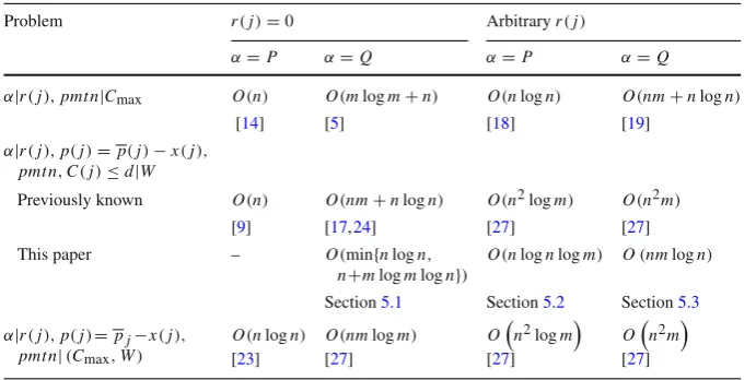
Zero release dates, common deadline The results for the models under these condi-tions are summarized in the second and third columns of Table 1. If the machines are identical, then solving problem P|pmt n|Cmaxwith fixed processing times can
be done by a linear-time algorithm that is due to McNaughton [14]. As shown by Jansen and Mastrolilli [9], problem P|p(j) = p(j)−x(j),pmt n,C(j) ≤ d|W reduces to a continuous generalized knapsack problem and can be solved in O(n) time. Shakhlevich and Strusevich [23] consider the bicriteria problem P|p(j) = p(j)−x(j),pmt n|(Cmax,W) ,in which makespanCmaxand the total compression
costW =w(j)x(j)have to be minimized simultaneously, in the Pareto sense; the running time of their algorithm isO(nlogn).
In the case of uniform machines, the best known algorithm for solving problem Q|pmt n|Cmax with fixed processing times is due to Gonzalez and Sahni [5]. For
problem Q|p(j) = p(j)−x(j),pmt n,C(j) ≤ d|W Nowicki and Zdrzałka [17] show how to find the actual processing times inO(nm+nlogn)time. Shakhlevich and Strusevich [24] reduce the problem to maximizing a linear function over a gener-alized polymatroid; they give an algorithm that requires the same running time as that by Nowicki and Zdrzałka [17], but can be extended to solving a bicriteria problem Q|p(j) = p(j)−x(j),pmt n|(Cmax,W). The best running time for the
bicrite-ria problem isO(nmlogm), which is achieved in [27] by submodular optimization techniques.
Table 1 Summary of the results
Problem r(j)=0 Arbitraryr(j)
α=P α=Q α=P α=Q
α|r(j),pmtn|Cmax O(n) O(mlogm+n) O(nlogn) O(nm+nlogn)
[14] [5] [18] [19]
α|r(j),p(j)=p(j)−x(j), pmtn,C(j)≤d|W
Previously known O(n) O(nm+nlogn) O(n2logm) O(n2m)
[9] [17,24] [27] [27] This paper – O(min{nlogn,
n+mlogmlogn})
O(nlognlogm) O(nmlogn)
Section5.1 Section5.2 Section5.3
α|r(j),p(j)=pj−x(j), pmtn|(Cmax,W)
O(nlogn) O(nmlogm) On2logm On2m
[23] [27] [27] [27]
be solved inO(nlogn)time (or inO(nlogm)time if the jobs are pre-sorted) as proved by Sahni [18]. For the uniform machines, Sahni and Cho [19] give an algorithm for problemQ|r(j),pmt n|Cmaxthat requiresO(mn+nlogn)time (orO(mn)time if
the jobs are pre-sorted).
Prior to our work on the links between submodular optimization and schedul-ing with controllable processschedul-ing times [27], no purpose-built algorithms have been known for problems α|r(j),p(j) = p(j) − x(j),pmt n,C(j) ≤ d|W with α ∈ {P,Q}. It is shown in [27] that the bicriteria problems αm|r(j),p(j) =
p(j)−x(j),pmt n|(Cmax,W)can be solved in O
n2logm time and in O(n2m) time for α = P andα = Q, respectively. Since a solution to a single criterion problemαm|r(j),p(j)=p(j)−x(j),pmt n,C(j)≤d|W is contained among the Pareto optimal solutions for the corresponding bicriteria problemαm|r(j),p(j)= p(j)−x(j),pmt n|(Cmax,W), the algorithms from [27] are quoted in Table1as the
best previously known for the single criterion problems with controllable processing times.
The main purpose of this paper is to demonstrate that the single criterion scheduling problems with controllable processing times to minimize the total compression cost can be solved by faster algorithms that are based on reformulation of these problems in terms of a linear programming problem over a submodular polyhedron intersected with a box. For the latter generic problem, we develop a recursive decomposition algorithm and show that for the scheduling applications it can be implemented in a very efficient way.
3 Scheduling with controllable processing times: submodular reformulations
problem for which the set of constraints is a submodular polyhedron intersected with a box. Being quite general, the problem represents a range of scheduling models with controllable processing times. In Sect.3.2we give the details of the corresponding reformulations.
3.1 Preliminaries on submodular polyhedra
For a positive integern, let N = {1,2, . . . ,n}be a ground set, and let 2N denote the family of all subsets of N. For a subset X ⊆ N, let RX denote the set of all vectors p with real components p(j), where j ∈ X. For two vectors p =
(p(1),p(2), . . . ,p(n))∈RNandq=(q(1),q(2), . . . ,q(n))∈RN, we writep≤q
ifp(j)≤q(j)for eachj ∈N. Given a setX ⊆RN, a vectorp∈ Xis calledmaximal inX if there exists no vectorq∈ Xsuch thatp≤qandp=q. For a vectorp∈RN, define p(X)=j∈X p(j)for every setX∈2N.
A set functionϕ:2N →Ris calledsubmodularif the inequality
ϕ(X)+ϕ(Y)≥ϕ(X∪Y)+ϕ(X∩Y)
holds for all sets X,Y ∈ 2N. For a submodular functionϕ defined on 2N such that ϕ(∅)=0, the pair(2N, ϕ)is called asubmodular systemonN, whileϕis referred to as therank functionof that system.
For a submodular system(2N, ϕ), define two polyhedra
P(ϕ)=p∈RN | p(X)≤ϕ(X), X∈2N
, (2)
B(ϕ)=p∈RN |p∈P(ϕ), p(N)=ϕ(N)
, (3)
called thesubmodular polyhedronand thebase polyhedron, respectively, associated with the submodular system. Notice thatB(ϕ)represents the set of all maximal vectors inP(ϕ).
The main problem that we consider in this section is as follows:
(LP): Maximize
j∈N
w(j)p(j)
subject to p(X)≤ϕ(X), X∈2N, p(j)≤ p(j)≤ p(j), j ∈N,
(4)
whereϕ :2N →Ris a submodular function withϕ(∅)=0,w∈R+Nis a nonnegative weight vector, andp,p∈ RN are upper and lower bound vectors, respectively. This problem serves as a mathematical model for many scheduling problems with control-lable processing times. Problem (LP) can be classified as a problem of maximizing a linear function over a submodular polyhedron intersected with a box.
have shown that a problem of maximizing a linear function over the intersection of a submodular polyhedron and a box is equivalent to maximizing the same objective function over a base polyhedron associated with another rank function.
Theorem 1 (cf. [25])
(i) Problem (LP) has a feasible solution if and only ifp∈ P(ϕ)andp≤p. (ii) If Problem (LP) has a feasible solution, then the set of maximal feasible solutions
of Problem (LP) is a base polyhedron B(ϕ)˜ associated with the submodular system (2N,ϕ), where the rank function˜ ϕ˜:2N→Ris given by
˜
ϕ(X)= min
Y∈2N
ϕ(Y)+p(X\Y)−p(Y\X)
. (5)
Notice that the computation of the value ϕ(X˜ )for a given X ∈ 2N reduces to minimization of a submodular function, which can be computed in polynomial time by using any of the available algorithms for minimizing a submodular function [7,20]. However, the running time of known algorithms is fairly large. In many special cases of Problem (LP), including its applications to scheduling problems with controllable processing times, the valueϕ(˜ X)can be computed more efficiently without using the submodular function minimization, as shown later.
Throughout this paper, we assume that Problem (LP) has a feasible solution, which, due to claim (i) of Theorem1, is equivalent to the conditionsp∈ P(ϕ)andp ≤p. Claim (ii) of Theorem1implies that Problem (LP) reduces to the following problem:
Maximize
j∈N
w(j)p(j)
subject to p∈ B(ϕ),˜
(6)
where the rank functionϕ˜:2N →Ris given by (5).
An advantage of the reduction of Problem (LP) to a problem of the form (6) is that the solution vector can be obtained essentially in a closed form, as stated in the theorem below.
Theorem 2 (cf. [4])Let j1,j2, . . . ,jnbe an ordering of elements in N that satisfies
w(j1)≥w(j2)≥ · · · ≥w(jn). (7)
Then, vectorp∗∈RNgiven by
p∗(jh)= ˜ϕ({j1, . . . ,jh−1,jh})− ˜ϕ({j1, . . . , jh−1}), h=1,2, . . . ,n, (8)
is an optimal solution to the problem(6)[and also to the problem(4)].
eachh = 1,2, . . . ,n. In this paper, instead, we use a different algorithm based on decomposition approach to achieve better running times for special cases of Problem (LP), as explained in Sect.4.
3.2 Rank functions for scheduling applications
In this subsection, we follow [27] and present reformulations of three scheduling problems on parallel machines with controllable processing times in terms of LP problems defined over a submodular polyhedron intersected with a box of the form (4). We assume that if the jobs have different release dates, they are numbered to satisfy
r(1)≤r(2)≤ · · · ≤r(n). (9)
If the machines are uniform they are numbered in accordance with (1). We denote
S0=0, Sk=s1+s2+ · · · +sk, 1≤k≤m. (10)
Skrepresents the total speed ofkfastest machines; if the machines are identical,Sk =k
holds.
For each problem Q|p(j)= p(j)−x(j),C(j)≤ d,pmt n|W, P|r(j),p(j)= p(j) − x(j),C(j) ≤ d,pmt n|W and Q|r(j),p(j) = p(j) − x(j),C(j) ≤ d,pmt n|W, we need to find the actual processing timesp(j)=p(j)−x(j), j ∈ N, such that all jobs can be completed by a common due datedand the total compression costW =j∈Nw(j)x(j)is minimized. In what follows, we present LP formulations of these problems withp(j), j ∈N, being decision variables, and the objective func-tion to be maximized being j∈Nw(j)p(j) = j∈Nw(j) (p(j)−x(j)). Since each decision variablep(j)has a lower bound p(j)and an upper boundp(j),an LP formulation includes the box constraints of the formp(j)≤ p(j)≤ p(j), j∈ N.
The derivations of the rank functions for the models under consideration can be justified by the conditions for the existence of a feasible schedule for a given common deadlined formulated, e.g., in [1]. Informally, these conditions state that for a given deadlined a feasible schedule exists if and only if
(i) for eachk,1≤k≤m−1,klongest jobs can be processed onkfastest machines by timed, and
(ii) allnjobs can be completed on allmmachines by timed.
We refer to [27] where the rank functions for the relevant problems are presented and discussed in more details. Below we present their definitions. In all scheduling applications a meaningful interpretation ofϕ(X)is the largest capacity available for processing the jobs of setX.
For example, problem Q|p(j) = p(j)−x(j),C(j) ≤ d,pmt n|W reduces to Problem (LP) of the form (4) with the rank function
ϕ(X)=d Smin{|X|,m}=
d S|X|, if |X| ≤m−1,
d Sm, if |X| ≥m.
It is clear that the conditionsp(X)≤ϕ(X),X ∈2N, for the functionϕ(X)defined by (11) correspond to the conditions (i) and (ii) above, provided that|X| ≤m−1 and
|X| ≥m, respectively. As proved in [24], functionϕis submodular.
We then consider problemQ|r(j),p(j)=p(j)−x(j),C(j)≤d,pmt n|W. For a set of jobs X ⊆ N, we defineri(X)to be thei-th smallest release date in set X ∈
2N,1≤i ≤ |X|. Then, for a non-empty setXof jobs, the largest processing capacity available on the fastest machine M1 is s1(d−r1(X)), the total largest processing
capacity on two fastest machinesM1andM2iss1(d−r1(X))+s2(d−r2(X)), etc.
We deduce that
ϕ(X)=
d S|X|−
|X|
i=1siri(X), if |X| ≤m−1,
d Sm−
m
i=1siri(X), if |X| ≥m.
(12)
It can be verified that this function is submodular.
Problem P|r(j),p(j) = p(j)−x(j),C(j) ≤ d,pmt n|W is a special case of problemQ|r(j),p(j)= p(j)−x(j),C(j)≤d,pmt n|W, wheres1=s2= · · · =
sm =1. Hence, the corresponding rank functionϕcan be simplified as
ϕ(X)=
d|X| −|iX=|1ri(X), if |X| ≤m−1,
dm−mi=1ri(X), if |X| ≥m.
(13)
4 Decomposition of LP problems with submodular constraints
In this section, we describe a decomposition algorithm for solving LP problems defined over a submodular polyhedron intersected with a box. In Sect.4.1, we demonstrate that the linear programming problem under study can be recursively decomposed into subproblems of a smaller dimension, with some components of a solution vector fixed to one of their bounds. We provide an outline of an efficient recursive decomposi-tion procedure in Sect.4.2and analyze its time complexity in Sect.4.3. In Sect.5
we present implementation details of the recursive decomposition procedure for the relevant scheduling models with controllable processing times.
4.1 Fundamental idea for decomposition
In this section, we show an important property, which makes the foundation of our decomposition algorithm for Problem (LP) of the form (4).
The lemma below demonstrates that some components of an optimal solution can be fixed either at their upper or lower bounds, while for some components their sum is fixed. Given a subsetNˆ of N, we say thatNˆ is aheavy-element subset of N with respect to the weight vectorwif it satisfies the condition
min
j∈ ˆN
w(j)≥ max
j∈N\ ˆN
w(j).
Given Problem (LP), in accordance with (5) define a set Y∗ ⊆ N such that the equality
˜
ϕ(X)=ϕ(Y∗)+p(X\Y∗)−p(Y∗\X) (14)
holds for a setX ⊆N. Because of its special role, in the remainder of this paper we callY∗aninstrumentalset for setX.
Lemma 1 LetNˆ ⊆N be a heavy-element subset of N with respect tow, and Y∗⊆N be an instrumental set for setN . Then, there exists an optimal solutionˆ p∗of Problem (LP) such that
(a)p∗(Y∗)=ϕ(Y∗),(b)p∗(j)= p(j), j∈ ˆN\Y∗,(c)p∗(j)= p(j), j ∈Y∗\ ˆN.
Proof Since Nˆ is a heavy-element subset, there exists an ordering j1,j2, . . . ,jn of
elements inNthat satisfies (7) andNˆ = {j1,j2, . . . ,jk}, wherek= | ˆN|. Theorems1
and2guarantee that the solutionp∗given by (8) is optimal. In particular, this implies
p∗(Nˆ)= ˜ϕ(j1)+
k
i=2
(ϕ(˜ {j1,j2, . . . ,ji})− ˜ϕ({j1,j2, . . . ,ji−1}))
= ˜ϕ({j1,j2, . . . ,jk})= ˜ϕ(Nˆ).
Sincep∗is a feasible solution of Problem (LP), the following conditions simultane-ously hold:
p∗(Y∗)≤ϕ(Y∗), p∗(j)≤ p(j), j ∈ ˆN\Y∗, −p∗(j)≤ −p(j),j∈Y∗\ ˆN. (15)
On the other hand, due to the choice of setY∗we have
p∗(N)ˆ = ˜ϕ(N)ˆ =ϕ(Y∗)+p(Nˆ\Y∗)−p
Y∗\ ˆN
,
which implies that each inequality of (15) must hold as equality, and that is equivalent
to the properties (a), (b), and (c) in the lemma.
In what follows, we use two fundamental operations on a submodular system
2N, ϕ , as defined in [4, Section 3.1]. For a set A ∈ 2N, define a set function ϕA:2A→Rby
ϕA(X)=ϕ(X),
X ∈2A.
Then,(2A, ϕA)is a submodular system onAand it is called arestriction of (2N, ϕ) to A. On the other hand, for a setA∈2Ndefine a set functionϕA:2N\A→Rby
Then,(2N\A, ϕA)is a submodular system onN\Aand it is called acontraction of
(2N, ϕ)by A.
For an arbitrary setA∈2N, Problem (LP) can be decomposed into two subproblems of a similar structure by performing restriction of 2N, ϕ to Aand contraction of
2N, ϕ byA, respectively. These problems can be written as follows: for restriction as
(LP1): Maximize
j∈A
w(j)p(j)
subject to p(X)≤ϕA(X)=ϕ(X), X ∈2A, p(j)≤ p(j)≤ p(j), j ∈ A,
and for contraction as
(LP2): Maximize
j∈N\A
w(j)p(j)
subject to p(X)≤ϕA(X)=ϕ(X∪A)−ϕ(A), X ∈2N\A,
p(j)≤ p(j)≤ p(j), j∈ N\A.
We show that an optimal solution of the original Problem (LP) can be easily restored from the optimal solutions of these two subproblems. For every subset A ⊆ N and vectorsp1∈RAandp2∈RN\A, thedirect sump1⊕p2∈RNofp1andp2is defined by
(p1⊕p2)(j)=
p1(j), if j ∈ A,
p2(j), if j ∈ N\A.
Lemma 2 Let A ∈ 2N, and suppose that q(A) = ϕ(A)holds for some optimal solutionq∈RNof Problem (LP). Then,
(i) Each of problems (LP1) and (LP2) has a feasible solution.
(ii) If a vectorp1∈ RAis an optimal solution of Problem (LP1) and a vectorp2 ∈
RN\Ais an optimal solution of Problem (LP2), then the direct sump∗=p1⊕p2∈
RNofp1andp2is an optimal solution of Problem (LP).
Proof The proof below is similar to that for Lemma 3.1 in [4]. We define vectors
q1∈RAandq2∈RN\Aby
q1(j)=q(j),j∈ A, q2(j)=q(j),j∈ N\A.
To prove (i), it suffices to show thatq1andq2are feasible solutions of Problems (LP1) and (LP2), respectively. Sinceqis a feasible solution of Problem (LP), we have
q(X)≤ϕ(X), X ∈2N, (16)
Then, (16) and (17) imply thatq1 ∈ RAis a feasible solution of Problem (LP1). It follows from (16) and the equalityq(A)=ϕ(A)that
q(X)=q(X∪A)−q(A)≤ϕ(X∪A)−ϕ(A), X ∈2N\A,
which, together with (17), implies thatq2 ∈RN\Ais a feasible solution of Problem (LP2). This concludes the proof of (i).
To prove (ii), we first show thatp∗is a feasible solution of Problem (LP). Sincep1
andp2are feasible solutions of Problem (LP1) and Problem (LP2), respectively, we have
p∗(X)≤ϕ(X), X ∈2A, (18)
p∗(X)≤ϕ(X∪A)−ϕ(A), X ∈2N\A, (19)
p(j)≤ p∗(j)≤ p(j), j ∈N. (20)
For anyX∈2N, we derive
p∗(X)= p∗(X∩A)+p∗(X\A)
≤ϕ(X∩A)+ϕ((X\A)∪A)−ϕ(A)
=ϕ(X∩A)+ϕ(X∪A)−ϕ(A)
≤ϕ(X),
where the first inequality is by (18) and (19), and the second by the submodularity of ϕ. This inequality and (20) show that the vectorp∗is a feasible solution of (LP).
To show optimality ofp∗, notice that by optimality ofp1andp2we have
j∈A
w(j)p1(j)≥
j∈A
w(j)q1(j),
j∈N\A
w(j)p2(j)≥
j∈N\A
w(j)q2(j),
and due to the definition ofp∗we obtain
j∈N
w(j)p∗(j)=
j∈A
w(j)p1(j)+
j∈N\A
w(j)p2(j)
≥
j∈A
w(j)q1(j)+
j∈N\A
w(j)q2(j) =
j∈N
w(j)q(j),
so that,p∗is an optimal solution of (LP).
From Lemmas1and2, we obtain the following property, which is used recursively in our decomposition algorithm.
(LPR): Maximize
j∈Y∗
w(j)p(j)
subject to p(X)≤ϕ(X), X∈2Y∗,
p(j)≤ p(j)≤ p(j), j ∈Y∗∩ ˆN, p(j)=p(j), j ∈Y∗\ ˆN
(LPC): Maximize
j∈N\Y∗
w(j)p(j)
subject to p(X)≤ϕ(X∪Y∗)−ϕ(Y∗), X ∈2N\Y∗, p(j)≤ p(j)≤ p(j), j ∈(N\Y∗)\
ˆ
N\Y∗
, p(j)=p(j), j ∈ ˆN\Y∗.
Then, the vectorp∗∈RNgiven by the direct sump∗=p1⊕p2is an optimal solution of (LP).
Notice that Problem (LPR) is obtained from Problem (LP) as a result of restriction toY∗and the values of components p(j),j ∈Y∗\ ˆN, are fixed to their lower bounds in accordance with Property (c) of Lemma1. Similarly, Problem (LPC) is obtained from Problem (LP) as a result of contraction byY∗ and the values of components p(j),j ∈ ˆN\Y∗, are fixed to their upper bounds in accordance with Property (b) of Lemma1.
4.2 Recursive decomposition procedure
In this subsection, we describe how the original Problem (LP) can be decomposed recursively based on Theorem 3, until we obtain a collection of trivially solvable problems with no non-fixed variables. In each stage of this process, the current LP problem is decomposed into two subproblems, each with a reduced set of variables, while some of the original variables receive fixed values and stay fixed until the end.
Remark 1 The definition of a heavy-element set can be revised to take into account the fact that some variables may become fixed during the solution process. The fixed variables make a fixed contribution into the objective function, so that the values of their weights become irrelevant for further consideration and can therefore be made, e.g., zero. This means that a heavy-element set can be selected not among all variables of set N but only among the non-fixed variables. Formally, if the set N of jobs is known to be partitioned asN = Q∪F, where the variables of setQare non-fixed and those of setF are fixed, then Qˆ ⊆ Qis aheavy-element subset with respect to the weight vectorwif it satisfies the condition
min
j∈ ˆQ
w(j)≥ max
j∈Q\ ˆQ
Notice that for this refined definition of a heavy-element subset, Lemma1and Theo-rem3can be appropriately adjusted.
In each stage of the recursive procedure, we need to solve a subproblem that can be written in the following generic form:
LP(H,F,K,l,u) Maximize
j∈H
w(j)p(j)
subject to p(X)≤ϕHK(X)=ϕ(X∪K)−ϕ(K), X ∈2H, l(j)≤ p(j)≤u(j), j ∈ H\F,
p(j)=u(j)=l(j), j ∈F,
(21)
where
– H⊆Nis the index set of components of vectorp;
– F ⊆ H is the index set of fixed components, i.e.,l(j) = u(j)holds for each j ∈F;
– K ⊆N\His the set that defines the rank functionϕKH :2H →Rsuch that
ϕH
K(X)=ϕ(X∪K)−ϕ(K), X ∈2H;
– l=(l(j)| j ∈ H)andu=(u(j)| j ∈ H)are respectively the vectors of the lower and upper bounds on variables p(j),j ∈ H. For j ∈ N, each ofl(j)and u(j)either takes the value ofp(j)or that ofp(j)from the original Problem (LP). Notice thatl(j)=u(j)for each j ∈F.
Throughout this paper, we assume that each Problem LP(H,F,K,l,u)is feasible. This is guaranteed by Lemma2if the initial Problem (LP) is feasible.
The original Problem (LP) is represented as Problem LP(N,∅,∅,p,p). Forj ∈ H, we say that the variablep(j)is anon-fixed variableifl(j) <u(j)holds, and afixed variableifl(j)= u(j)holds. If all the variables in Problem LP(H,F,K,l,u)are fixed, i.e.,l(j) = u(j)holds for all j ∈ H, then an optimal solution is uniquely determined by the vectoru∈RH.
Consider a general case that Problem LP(H,F,K,l,u)of the form (21) contains at least one non-fixed variable, i.e.,|H\F|>0. We define a functionϕKH :2H →R by
ϕH
K(X)= min Y∈2H{ϕ
H
K(Y)+u(X\Y)−l(Y\X)}. (22)
By Theorem1(ii), the set of maximal feasible solutions of Problem LP(H,F,K,l,u)
is given as a base polyhedronB(ϕKH)associated with the functionϕKH. Therefore, if
|H\F| =1 andH\F = {j}, then an optimal solutionp∗∈RH is given by
p∗(j)=
˜
ϕH
K({j}), j = j,
Suppose that|H\F| ≥2. Then, we call a procedure ProcedureDecomp(H,F,K,
l,u)explained below. LetHˆ ⊆H\Fbe a heavy-element subset ofHwith respect to the vector(w(j)| j ∈ H), andY∗⊆Hbe an instrumental set for setH, i.e.,ˆ
ϕH
K(Hˆ)=ϕKH(Y∗)+u
ˆ
H\Y∗
−l(Y∗\ ˆH). (24)
Theorem3, when applied to Problem LP(H,F,K,l,u), implies that the problem
is decomposed into the two subproblems
Maximize
j∈Y∗
w(j)p(j)
subject to p(X)≤ϕYK∗(X)=ϕ(X∪K)−ϕ(K), X ∈2Y∗, l(j)≤ p(j)≤l(j), j ∈Y∗\ ˆH, l(j)≤ p(j)≤u(j), j ∈Y∗∩ ˆH,
and
Maximize
j∈H\Y∗
w(j)p(j)
subject to p(X)≤ϕKH∪\YY∗∗(X)=ϕ(X∪K ∪Y∗)−ϕ(K∪Y∗), X∈2H\Y∗,
u(j)≤p(j)≤u(j), j∈ ˆH\Y∗,
l(j)≤p(j)≤u(j), j∈(H\Y∗)\(Hˆ\Y∗).
The first of these subproblems corresponds to Problem (LPR), and in that problem the values of components p(j),j ∈ Y∗\ ˆH, are fixed to their lower bounds. The second subproblem corresponds to Problem (LPC), and in that problem the values of components p(j),j ∈ ˆH\Y∗, are fixed to their upper bounds.
We denote these subproblems by Problem LP(Y∗,F1,K,l1,u1) and
Prob-lem LP(H\Y∗,F2,K∪Y∗,l2,u2), respectively, where the vectorsl1,u1∈RY∗ and l2,u2∈RH\Y∗, and the updated sets of fixed variablesF1andF2are given by
l1(j)=l(j),j ∈Y∗,
u1(j)=
l(j), j∈Y∗\ ˆH, u(j), j∈Y∗∩ ˆH, F1=Y∗\ ˆH,
(25)
l2(j)=
u(j), j∈ ˆH\Y∗, l(j), j∈ H\(Y∗∪ ˆH), u2(j)=u(j),j ∈H\Y∗,
F =(Hˆ ∪(H∩F))\Y .
Notice that Problem LP(Y∗,F1,K,l1,u1)inherits the set of fixed variablesY∗∩F
from the problem of a higher level, and additionally the variables of setY∗\ ˆHbecome fixed. However, since Hˆ contains only non-fixed variables, we deduce thatY∗\ ˆH ⊇ Y∗∩F, so that the complete description of the setF1of fixed variables in Problem
LP(Y∗,F1,K,l1,u1)is given byY∗\ ˆH.
Problem LP(H\Y∗,F2,K∪Y∗,l2,u2)inherits the set of fixed variables(H\Y∗)∩F
from the problem of a higher level, and additionally the variables of setHˆ\Y∗become fixed. These two sets are disjoint. Thus, the complete description of the setF2of fixed
variables in Problem LP(H\Y∗,F2,K,l2,u2)is given by(Hˆ ∪(H∩F))\Y∗.
Without going into implementation details, we now give a formal description of the recursive procedure, that takes Remark 1 into account. For the current Problem LP(H,F,K,l,u), we compute optimal solutions p1 ∈ RY∗ and p2 ∈ RH\Y∗of the two subproblems by calling proceduresDecomp(Y
∗,F1,K,l1,u1)and
Decomp(H\Y∗,F2,K∪Y∗,l2,u2). By Theorem3, the direct sump∗=p1⊕p2is an
optimal solution of Problem LP(H,F,K,l,u), which is the output of the procedure
Decomp(H,F,K,l,u).
ProcedureDecomp(H,F,K,l,u)
Step 1. If|H\F| =0, then output the vectorp∗=u∈RH and return.
If|H\F| =1 andH\F = {j}, then compute the valueϕ˜KH({j}), and output the vectorp∗given by (23) and return.
Step 2. Select a heavy-element subsetHˆ of H\F with respect tow, and determine an instrumental setY∗⊆Hfor setHˆ satisfying (24).
Step 3. Define the vectorsl1,u1∈RY∗and setF1by (25).
Call ProcedureDecomp(Y∗,F1,K,l1,u1)to obtain an optimal solutionp1∈RY∗
of Problem LP(Y∗,F1,K,l1,u1).
Step 4. Define the vectorsl2,u2∈RH\Y∗and setF2by (26).
Call ProcedureDecomp(H\Y∗,F2,K∪Y∗,l2,u2)to obtain an optimal solution p2∈RH\Y∗of Problem LP(H\Y∗,F2,K∪Y∗,l2,u2).
Step 5. Output the direct sump∗=p1⊕p2∈RH and return.
Recall that the original Problem (LP) is solved by calling Procedure Decomp(N,∅,∅,p,p). Its actual running time depends on the choice of a
heavy-element subsetHˆin Step 2 and on the time complexity of finding an instrumental setY∗.
4.3 Analysis of time complexity
We analyze the time complexity of ProcedureDecomp. To reduce the depth of recur-sion of the procedure, it makes sense to perform decomposition in such a way that the number of non-fixed variables in each of the two emerging subproblems is roughly a half of the number of non-fixed variables in the current Problem LP(H,F,K,l,u).
variables in each of the two subproblems that emerge as a result of decomposition is either|H\F|/2or|H\F|/2.
Proof For Problem LP(H,F,K,l,u), letg= |H\F|denote the number of the non-fixed variables. In Step 2 ProcedureDecomp(H,F,K,l,u)selects a heavy-element subset Hˆ ⊂ H\F that containsg/2non-fixed variables, i.e.,| ˆH| = g/2. Then, the number of the non-fixed variables in Problem LP(Y∗,F1,K,l1,u1)considered in
Step 3 satisfies|Y∗∩ ˆH| ≤ g/2.
Due to (26), the number of non-fixed variables in Problem LP(H\Y∗,F2,K ∪
Y∗,l2,u2)considered in Step 4 satisfies
|H\(Hˆ ∪F∪Y∗)| ≤ |H\ ˆH| =
g
2
.
This lemma implies that the overall depth of recursion of ProcedureDecompapplied to Problem LP(N,∅,∅,p,p)isO(logn).
Let us analyze the running time of Procedure Decomp applied to Problem LP(H,F,K,l,u). We denote by TLP(h,g) the time complexity of Procedure
Decomp(H,F,K,l,u), where h = |H| and g = |H\F|. Let TY∗(h)denote the
running time for computing the valueϕKH(H)ˆ for a given set Hˆ ⊆H and finding an instrumental setY∗that minimizes the right-hand side of the Eq. (22). In Steps 3 and 4, ProcedureDecompsplits Problem LP(H,F,K,l,u)into two subproblems: one with h1variables among which there existg1≤min{h1,g/2}non-fixed variables, and the
other one withh2=h−h1variables, among which there existg2≤min{h2,g/2}
non-fixed variables. LetTSplit(h)denote the time complexity of such a decomposition,
i.e., for setting up the instances of the two subproblems. A required heavy-element set can be found inO(h)time by using a linear-time median-finding algorithm. Then, we obtain a recursive equation:
TLP(h,g)=
⎧ ⎪ ⎨ ⎪ ⎩
O(1), ifg =0,
TY∗(h), ifg =1,
TY∗(h)+TSplit(h)+TLP(h1,g1)+TLP(h2,g2), ifg >1.
By solving the recursive equation under an assumption that both functionsTY∗(h)and
TSplit(h)are non-decreasing and convex, we obtain
TLP(n,n)=O(
TY∗(n)+TSplit(n) logn).
Thus, the findings of this section can be summarized as the following statement.
Theorem 4 Problem (LP) can be solved by Procedure Decomp in O((TY∗(n)+
TSplit(n))logn)time.
required set Y∗ in all levels of the recursive ProcedureDecomp. We develop fast algorithms that compute the value ϕ(Hˆ)and find a setY∗ in accordance with its definition; see Sect.5.
4.4 Comparison with decomposition algorithm for maximizing a concave separable function
In this subsection, we refer to our decomposition algorithm for Problem (LP) defined over a submodular polyhedron intersected with a box as Algorithm SSS-Decomp. Below, we compare that algorithm with a known decomposition algorithm that is applicable for maximizing a separable concave function over a submodular polyhe-dron; see [3], [4, Sect. 8.2] and [6].
Consider the problem of maximizing a separable concave function over a submod-ular polyhedron:
(SCFM) Maximize
j∈N
fj(p(j))
subject to p(X)≤ϕ(X), X ∈2N,
where fj :R→Ris a univariate concave function for j ∈ N andϕ:2N →Ris a
submodular function withϕ(∅)=0.
The decomposition algorithm for Problem (SCFM) was first proposed by Fujishige [3] for the special case where each fj is quadratic and ϕ is a
polyma-troid rank function. Groenevelt [6] then generalized the decomposition algorithm for the case where each fj is a general concave function andϕ is a polymatroid rank
function. Later, it was pointed out by Fujishige [4, Sect. 8.2] that the decomposition algorithm in [6] can be further generalized to the case whereϕis a general submodular function. We refer to that algorithm as Algorithm FG-Decomp.
For simplicity of presentation, in the description of Algorithm FG-Decomp we assume that each fj is monotone increasing; the general case with non-monotone fj
can be dealt with by an appropriate modification of the algorithm; see [6].
Algorithm FG-Decomp
Step 1. Find an optimal solutionq∈RN of the following “relaxed” problem with a single constraint:
Maximize
j∈N
fj(p(j))
subject to p(N)≤ϕ(N).
Note: since fj is monotone it follows thatq(N)=ϕ(N).
Step 2. Find a maximal vectorq∈RNsatisfying the following condition: q(X)≤ϕ(X), X ∈2N, q(j)≤q(j), j ∈ N.
Step 4. IfY∗=N, then output the vectorqand stop. Otherwise, go to Step 5. Step 5. Find an optimal solutionp1∈RY∗of the following problem:
Maximize
j∈Y∗
fj(p(j))
subject to p(X)≤ϕ(X),X ∈2Y∗.
Step 6. Find an optimal solutionp2∈RN\Y∗of the following problem:
Maximize
j∈N\Y∗
fj(p(j))
subject to p(X)≤ϕ(X∪Y∗)−ϕ(Y∗), X ∈2N\Y∗.
Step 7. Output the direct sump∗=p1⊕p2∈RNand stop.
Notice that for the setY∗chosen in Step 3, there exists some optimal solutionp∗
of Problem (SCFM) such thatϕ(Y∗)=p∗(Y∗); see [4, Sect. 8.2], [6].
It is easy to see that Problem (LP) can be reduced to Problem (SCFM) by setting the functions fj as
fj(α)=
⎧ ⎪ ⎨ ⎪ ⎩
w(j)p(j)+M(α−p(j)), if α < p(j); w(j)α, if p(j)≤α≤ p(j); w(j)p(j)−M(α−p(j)), if α > p(j)
(27)
with a sufficiently large positive number M. Thus, Algorithm FG-Decomp (appro-priately adjusted to deal with non-monotone functions fj) can be applied to solving
Problem (LP).
For Problem (LP), Algorithm FG-Decomp is quite similar to Algorithm SSS-Decomp. Indeed, both algorithms recursively find a setY∗and decompose a problem into two subproblems by using restriction toY∗and contraction byY∗.
The difference of the two decomposition algorithms is in the selection rule of a set Y∗. In fact, a numerical example can be provided that demonstrates that for the same instance of Problem (LP) the two decomposition algorithms may find different sets Y∗in the same iteration.
In addition, Algorithm SSS-Decomp fixes some variables in the subproblems so that the number of non-fixed variables in each subproblem is at most the half of the non-fixed variables in the original problem; this is an important feature of our algorithm which is not enjoyed by Algorithm FG-Decomp. This difference affects the efficiency of the two decomposition algorithms; indeed, for Problem (LP) the height of the decomposition tree can beΘ(n)if Algorithm FG-Decomp is used, while it is O(logn)in our Algorithm SSS-Decomp.
On the other hand, assume that the feasible region for Problem (SCFM) is addi-tionally restricted by imposing the box constraints, similar to those used in Problem (LP). Theorem1can be used to reduce the resulting problem to Problem (SCFM) with a feasible region being the base polyhedron with a modified rank function. Although the obtained problem can be solved by Algorithm FG-Decomp, this approach is com-putationally inefficient, since it requires multiple calls to a procedure for minimizing a submodular function. It is more efficient not to rely on Theorem1, but to handle the additional box constraints by adapting the objective function, similarly to (27), and then to use Algorithm FG-Decomp.
5 Application to parallel machine scheduling problems
In this section, we show how the decomposition algorithm based on ProcedureDecomp can be adapted for solving problems with parallel machines efficiently. Before con-sidering implementation details that are individual for each scheduling problem under consideration, we start this section with a discussion that addresses the matters that are common to all three problems.
Recall that each scheduling problem we study in this paper can be formulated as Problem (LP) of the form (4) with an appropriate rank function. Thus, each of these problems can be solved by the decomposition algorithm described in Sect.4.2applied to Problem LP(N,∅,∅,l,u), wherel=pandu=p.
For an initial Problem LP(N,∅,∅,l,u), we assume that the following preprocessing is done before calling ProcedureDecomp(N,∅,∅,l,u):
1. If required, the jobs are numbered in non-decreasing order of their release dates in accordance with (9).
2. If required, the machines are numbered in non-increasing order of their speeds in accordance with (1), and the partial sumsSvare computed for allv,0≤v≤m, by (10).
3. The lists(l(j)| j ∈N)and (u(j)| j∈ N)are formed and their elements are sorted in non-decreasing order.
The required preprocessing takesO(nlogn)time.
To adapt the generic Procedure Decomp to solving a particular schedul-ing problem, we only need to provide the implementation details for Procedure Decomp(H,F,K,l,u)that emerges at a certain level of recursion. To be precise, we need to explain how to compute for each particular problem the functionϕKH(X) for a chosen setX ∈2H and how to find for a current heavy-element set an instru-mental setY∗defined by (22), which determines the pair of problems into which the current problem is decomposed.
Given Problem LP(H,F,K,l,u)of the form (21) defineh = |H|andk = |K|. Recall thatK,H ⊆Nare sets withK ∩H = ∅. Forv=0,1, . . . ,h, define
Introduce
ˆ
h =min{h,m−k−1}. (29)
Since ϕKH(Y) = ϕ(Y ∪K)−ϕ(K)for Y ∈ 2H, it follows that for a given set X ⊆Hthe functionϕKH :2H →Rcan be computed as follows:
ϕH
K(X)= min Y∈2H
ϕH
K(Y)+u(X\Y)−l(Y\X)
=u(X)−ϕ(K)+ min
Y∈2H{ϕ(Y∪K)−u(Y ∩X)−l(Y\X)}
=u(X)−ϕ(K)+ min
Y∈2H{ϕ(Y∪K)−λ(Y)}, (30) where ϕ is the initial rank function associated with the scheduling problem under consideration, and
λ(j)=
u(j), if j ∈ X,
l(j), if j ∈ H\X. (31)
Notice that if the minimum in the left-hand side of (30) is achieved forY =Y∗, thenY∗is an instrumental set for setX.
5.1 Uniform machines, equal release dates
In this subsection, we show that problemQ|p(j)=p(j)−x(j),C(j)≤d,pmt n|W can be solved inO(nlogn)time by the decomposition algorithm. To achieve this, we consider Problem LP(H,F,K,l,u)that arises at some level of recursion of Proce-dureDecompand present a procedure for computing the functionϕH
K : 2H → R
given by (22). We show that for an arbitrary set X ⊆ H the value ϕKH(X)can be computed inO(h)time. For a heavy-element set Hˆ ⊆ H\F, finding a setY∗that is instrumental for setHˆ also requiresO(h)time.
Recall that for problem Q|p(j) = p(j)−x(j),C(j) ≤ d,pmt n|W the rank functionϕ:2N→Ris defined by (11), i.e.,
ϕ(X)=d Smin{m,|X|}, X ∈2N.
This, together with (30), implies
ϕH
K(X)=u(X)−d Smin{m,k}+ min Y∈2H
d Smin{m,|Y|+k}−λ(Y)
. (32)
Φ=
min
0≤v≤ ˆh
d Sv+k−max Y∈Hvλ(Y)
, if m>k,
+∞, if m≤k,
(33)
and
Φ=
d Sm−max{λ(Y)|Y ∈2H, |Y|>hˆ}, if h >m−k−1,
+∞, if h ≤m−k−1. (34)
Then, we can rewrite the last term in (32) as
min
Y∈2H{d Smin{m,|Y|+k}−λ(Y)} =min
Φ, Φ.
Notice thatΦ= +∞corresponds to the case that the setY ∈Hvdoes not exist for 0≤v ≤ ˆh(this happens ifm≤kor equivalentlyhˆ <0);Φ= +∞corresponds to the case that the setY ∈Hvdoes not exist forv >hˆ(this happens ifh≤m−k−1 or equivalentlyhˆ =h).
Assumem>k, and letλvbe thev-th largest value in the list(λ(j)| j ∈H)for v=1,2, . . . ,h. It follows thatˆ
Φ= min
0≤v≤ ˆh
d Sv+k−
v
i=1
λi
. (35)
We then assumeh >m−k−1. Sinceλ(j)≥0 for j ∈ H, the maximum in the right-hand side of the top line of (34) is achieved forY =H, i.e.,
Φ=d Sm−λ(H). (36)
Below we describe the procedure that uses Eqs. (35) and (36) for computing the valuesΦandΦ. Since the procedure will be used as a subroutine within the recursive ProcedureDecomp, here we present it for computingϕHK(X)withX being a heavy-element setH. Besides, its output contains setˆ Y∗,an instrumental set for setHˆ. Procedure CompQr0
Input: Problem LP(H,F,K,l,u), a heavy-element set Hˆ ⊆ H\F, the values of h,kandhˆdefined by (29), and the list(λ(j)| j ∈ H)computed by (31) with respect toX= ˆH.
Output: the value of functionϕKH(X)and an instrumental setY∗for setX = ˆH. Step 1. Ifk≥m, then setΦ:= +∞and go to Step 3.
Step 2. Do the following:
Step 2-1. Forv=1,2, . . . ,h, compute theˆ v-th largest valueλvamong the num-bersλ(j), j∈ H.
Step 2-2. Compute the valueΦby using (35). IfΦ=d Sv+k−
v
i=1λifor some