RCC*-9 and CBM*

This is a repository copy of

RCC*-9 and CBM*

_.

White Rose Research Online URL for this paper:

http://eprints.whiterose.ac.uk/83877/

Version: Accepted Version

Proceedings Paper:

Clementini, E and Cohn, AG (2014) RCC*-9 and CBM*. In: Duckham, M, Pebesma, E,

Stewart, K and Frank, AU, (eds.) Geographic Information Science 8th International

Conference, GIScience 2014, Proceedings. Geographic Information Science 8th

International Conference, GIScience 2014, 24-26 Sept 2014, Vienna, Austria. Springer ,

349 - 365. ISBN 978-3-319-11592-4

Reuse

Unless indicated otherwise, fulltext items are protected by copyright with all rights reserved. The copyright exception in section 29 of the Copyright, Designs and Patents Act 1988 allows the making of a single copy solely for the purpose of non-commercial research or private study within the limits of fair dealing. The publisher or other rights-holder may allow further reproduction and re-use of this version - refer to the White Rose Research Online record for this item. Where records identify the publisher as the copyright holder, users can verify any specific terms of use on the publisher’s website.

Takedown

If you consider content in White Rose Research Online to be in breach of UK law, please notify us by

RCC*-9 and CBM*

Eliseo Clementini1 and Anthony G. Cohn2

1

University of L’Aquila, Information Engineering, L’Aquila, Italy

[email protected] 2

University of Leeds, School of Computing, Leeds, UK

[email protected]

Abstract. In this paper we introduce a new logical calculus of the Region

Con-nection Calculus (RCC) family, RCC*-9. Based on nine topological relations, RCC*-9 is an extension of RCC-8 and models topological relations between multi-type geometric features: therefore, it is a calculus that goes beyond the modeling of regions as in RCC-8, being able to deal with lower dimensional features embedded in a given space, such as linear features embedded in the plane. Secondly, the paper presents a modified version of the Calculus-Based Method (CBM), a calculus for representing topological relations between spa-tial features. This modified version, called CBM*, is useful for defining a rea-soning system, which was difficult to define for the original CBM. The two new calculi RCC*-9 and CBM* are introduced together because we can show that, even if with different formalisms, they can model the same topological configu-rations between spatial features and the same reasoning strategies can be ap-plied to them.

1

Introduction

The RCC family of calculi [8] uses a logical approach for the representation of quali-tative topological relations. The calculi were developed with regions as the primitive spatial entity and the connection relation as the primitive topologic relation between regions, from which other relations can be defined. RCC-8, the most representative calculus of the family, can model eight topological relations between regions of the plane: there is a one-to-one correspondence with the eight topological relations that are definable with the 9IM between 2D simple regions. As remarked in [18], there exist few attempts to express topological relations between features of lower dimen-sions than the embedding space, such as lines in R2, due to the difficulties of dealing with different types. In [19], Galton introduced an axiomatic system for multidimen-sional mereotopology, using primitives for ‘part’ (P) and ‘boundary’ (B). Gott’s “INCH” calculus dealt with closed sets of points of uniform dimensionality [21] using a single primitive binary relation INCH (“includes a chunk of”). See further analysis in [9].

CBM [5] is a model for expressing topological relations between regions, lines, and points. It was especially defined for expanding the querying capabilities of data-base query languages towards spatial data. The operators of CBM have been adopted by the Open GeoSpatial Consortium (OGC) [23] and implemented in all spatial data-base systems. CBM relations can find an equivalent expression in terms of Egenhofer matrix-based methods [15] and vice versa. In particular, as it was shown in [3], CBM is more expressive than 9IM and equivalent to the Dimensionally-Extended 9-Intersection Model (DE+9IM) [3]. Despite its success in spatial databases and in the standardization process, CBM had little impact in the Qualitative Spatial Reasoning (QSR) community, due to the absence of a strong logical formulation and in particular its lack of composition tables. As pointed out in [16, 22], CBM is difficult to compare to logical calculi such as the RCC and no reasoning rules have been defined for it. The definitions of CBM were dependent on the dimension of the features participat-ing in the relation. For example, a cross between a line and a region had a different definition from a cross between two lines. This meant it was not possible to find a single composition table for the calculus: at best, it would have been possible to find composition tables for each group of relations, that is, for region/region relations, for line/region relations, and so on, as proposed in [22].

In this paper, we aim at establishing a bridge between RCC and CBM, by defining an extension of RCC-8 that is capable of modeling topological relations between spa-tial features of any dimensionality and an extension of CBM that is capable of reason-ing. To achieve this goal, a new calculus of the RCC family is defined, called RCC*-9, able to deal with features of various dimensions, not just regions1. A modification of CBM, called CBM*, is introduced that maps straightforwardly onto calculi of the RCC family and allows a composition table for reasoning to be found. Finally, it is shown that the two new calculi, RCC*-9 and CBM*, are able to model the same

1

logical configurations, even though they are defined in different ways, and they are compared with 9IM.

In Section 2, we recapitulate the definition of the geometric data model on which we base our work. In Section 3, we briefly recall the definitions of CBM. In Section 4, we introduce CBM* and discuss the changes between CBM and CBM*. In Section 5, we introduce the logical calculus RCC*-9. In Section 6, we define the spatial rea-soning system of both RCC*-9 and CBM*. In Section 7, we discuss how to express CBM* relations and RCC*-9 relations in terms of 9IM. In Section 7, we make some concluding remarks.

2

Definition of geometric features

In this paper, we will adopt the same terminology of the OGC where various point-sets of the plane R2 are called features, distinguishing between simple features and complex features [23]. The OGC simple feature model definitions were in turn taken from [4]. In the following, we briefly recall those definitions. First of all, features are classified with respect to their dimension: regions of dimension 2, lines of dimension 1, and points of dimension 0.

Let x be a two-dimensional point-set.

Def. 1. The interior x° of x is defined as the union of all open sets contained in x. Def. 2. The closure x of x is defined as the intersection of all closed sets containing x.

Def. 3. The boundary ∂x of x is defined as the set difference between its closure and its interior, i.e., x °.

Def. 4. The exterior x of x is defined as the set difference R2 \ x. Def. 5. x is regular closed if x=x°.

Def. 6. A simple region is a regular closed (non-empty) two-dimensional point-set x with a connected interior and connected exterior.

Def. 6 implies that a simple region is homeomorphic to the closed unit disk. A simple region does not have holes and is connected. If we remove the constraint of connected exterior from the definition, we obtain regions with holes [13]. In OGC simple feature specifications, regions with holes are implemented with the Polygon spatial data type. If we remove the constraint of connected interior, we obtain com-plex regions, that is, regions with holes and separations. Comcom-plex regions are imple-mented in OGC feature model with the MultiPolygon spatial data type.

Def. 7. A simple line is a closed (non-empty) one-dimensional point-set x defined as the image of a continuous mapping f:[0,1] → R2, such that ∀ , ∈[0,1], ≠ , f( )≠f( ).

Topologically, a simple line embedded in R2, being a one-dimensional set, has an empty interior. As common practice in GIS [15] and in OGC standards as well, the boundary ∂x of a line x is considered to be the set of its endpoints and the interior of the line the difference, x°=x \ ∂x. In this paper, we will adopt these definitions of boundary and interior of a line feature. In OGC feature model, simple lines are im-plemented with the Polyline spatial data type.

From Def. 7, if we remove the constraint of no self-intersections, we obtain lines with self-intersections. A particular case of a line with self-intersections is the closed ring, where f(0)=f(1). If a one-dimensional point set can be obtained as the union of several mappings from the unit interval to the plane, then we obtain the concept of a complex line. A complex line can be made of several disjoint components. A complex line in OGC feature model is implemented with the MultiPolyline spatial data type.

A simple point is a zero-dimensional element of the embedding space. A complex point is the union of a finite number of simple points. Following the OGC convention, we assume that point features have an empty boundary. Simple and complex point features are implemented in OGC standards with the Point and Multipoint spatial data types, respectively.

3

CBM

One of the basic ideas behind CBM [5] was to provide an easy spatial extension of the tuple relational calculus [7] to express queries such as:

{x| ∃y [River(x) ∧ Region(y) ∧ cross(x,y) ∧ y= ‘Abruzzo’]}

The above CBM expression corresponds to the query “Retrieve all the rivers that cross the Abruzzo region”. The topological relations of CBM can be applied not only to simple variables but to the boundaries of geometric features. Boundaries are ex-tracted by the three operators b (boundary – the closed line representing the boundary of a simple region), f (from – the first endpoint of a line), t (to – the second endpoint of a line) 2. For example, the following queries can be expressed in CBM:

{x| ∃y∃z [River(x) ∧ Mountain(y) ∧ Sea(z) ∧ in(f(x),y) ∧ y= ‘Apennines’ ∧ touch(t(x),z) ∧ z= ‘Adriatic’]}

{x| ∃y [Road(x) ∧ Region(y) ∧ cross(x,y) ∧ overlap(x,b(y)) ∧ y= ‘Abruzzo’]} The above expressions correspond to “Retrieve all the rivers that rise in the Apen-nines mountains and flow into the Adriatic sea” and “Retrieve all the roads that cross the Abruzzo region and have a part of the road along the region’s boundary”.

The five topological relations of CBM are named disjoint, touch, in, cross, overlap. The definition of these relations are (the ‘dim’ operator evaluates to 0, 1, 2 depending whether the argument is a 0-, 1-, or 2-dimensional point set):

Def. 8. disjoint(x,y) =def x∩y=∅ 2

Def. 9. touch(x,y) =def x°∩y°=∅ ∧ x∩y≠∅ Def. 10. in(x,y) =def x∩y=x ∧ x°∩y°≠∅

Def. 11. cross(x,y) =def dim(x°∩y°) < max(dim(x°),dim(y°)) ∧ x∩y≠x ∧ x∩y≠y Def. 12. overlap(x,y) =def dim(x°∩y°) = dim(x°) = dim(y°) ∧ x∩y≠x ∧ x∩y≠y The relations can be applied to all geometric types, either simple or complex [4]. They were implemented by the OGC feature model as a set of functions with names

Disjoint, Touches, Within, Crosses, Overlaps. Additionally, the con-verse function of Within was called Contains and the function Equals was defined as Within and Contains at the same time [23]. An expression of the relational tuple calculus extended with the five topological relations and the three boundary operators can be expressed by the Egenhofer matrix-based methods. Conversely, any instance of the DE+9IM can be expressed by an expression of CBM [3].

4

CBM*

In this section, we introduce a modification of CBM, called CBM*, for which it is easier to find an equivalence in terms of calculi of the RCC family and to find a com-position table for reasoning. The basic relations of CBM* have a slightly different meaning from the corresponding relations of CBM. We assume the following defini-tions (we adopt the same names followed by a *) accompanied by a qualitative expla-nation of the meaning:

Def. 13. disjoint*(x,y), the two features are disjoint: disjoint*(x,y) =def x∩y=∅

Def. 14. touch*(x,y), the two features intersect, but their interiors are disjoint (and it excludes containment):

touch*(x,y) =def x°∩y°=∅ ∧ x∩y≠∅ ∧ x∩y≠x ∧ x∩y≠y Def. 15. in*(x,y), feature x is part of feature y (it excludes equality):

in*(x,y) =def x∩y=x ∧ x≠y in*−1(x,y) =def x∩y=y ∧ x≠y equal*(x,y) =def x=y

Def. 16. cross*(x,y), the interiors of the two features intersect, but at least one fea-ture’s boundary does not intersect the other feature:

cross*(x,y) =def x°∩y°≠∅ ∧ (∂x∩y=∅ ∨ x∩∂y=∅)

Def. 17. overlap*(x,y): the interiors of the two features intersect and also each feature’s boundary intersects the other feature (and it excludes containment).

CBM*. The cross* and overlap* relations take into account the remaining cases with a different criterion for partitioning the cases with respect to the original cross and overlap relations. In Fig. 2, we can see the differences with some representative con-figurations. The overlap relation between a region and a line was not possible in CBM, while the relation overlap* between a region and a line corresponds to a real case.

Fig. 1. Decision tree for the relations of CBM*.

Fig. 2. Some differences between CBM and CBM* relations.

5

Definition of RCC*-9

In Cohn and his coauthors’ work, the spatial primitive entities of the calculus are regions [8, 11]. The primitive spatial entities of the proposed calculus RCC*-9 are instead generic spatial features, without forcing an interpretation in terms of regions, lines, or points. As discussed in Section 2, in topology a feature of co-dimension big-ger than zero (such as a line or a point in R2) does not have an interior. One conse-quence is that a line in R2 cannot have a non-tangential proper part (see also Galton’s work [18]). The RCC definitions work when the universe of discourse contains

re-F x∩y=∅ T

disjoint* x=y

T

equal* x∩y=x

T

in* x∩y=y

T

in*−1 x°∩y°=∅

touch* ∂x∩y=∅∨ x∩∂y=∅

cross* overlap*

F

F F

F

T T

F

T

touch

in*

cross

overlap*

cross

cross*

cross

cross*

overlap

cross

overlap

gions of dimension Rn, for any n>0. But the definitions do not work for points or for universes of discourse containing regions of mixed dimensionality3.

The boundary of an interval is made up of its two endpoints. A non-tangential proper part of an interval is another interval that is inside the first one and that does not connect with the endpoints of the first one. Adopting the “usual” GIS definitions [4, 15], non-tangential proper parts of lines embedded in R2 can be defined as a map-ping from one-dimensional intervals to the plane. In this way, we can find RCC*-9 definitions of topological relations that apply to all kinds of spatial features.

Analogously to RCC-8, we consider a primitive connected relation between two features C(x,y). There are several models for RCC in the literature; here, for con-sistency with CBM*, we take our universe of discourse to be closed regions (possibly disconnected), closed lines (also possibly disconnected), and sets of isolated points. C(x,y) is interpreted as being true when x and y have at least one point in common. The connected relation enjoys two axioms:

C(x,x),

C(x,y)→C(y,x).

From the primitive connected relation, other relations are consequently defined. These are as in RCC8 except as noted. The disconnected relation is defined as:

Def. 18. DC(x,y) =def ¬C(x,y)

The part relation between x and y is defined by saying that the feature x cannot be connected to features disconnected from y:

Def. 19. P(x,y) =def ∀z [C(z,x)→C(z,y)]

The proper part relation excludes the case of equality between the two features: Def. 20. PP(x,y) =def P(x,y) ∧¬P(y,x)

The equal relation is defined as:

Def. 21. EQ(x,y) =def P(x,y) ∧P(y,x)

In the original RCC, the overlap relation was defined as: O(x,y) = ∃z [P(z,x) ∧ P(z,y)]. Such a definition sufficed to refine the connected relation and make a distinc-tion between the overlap and the externally connected reladistinc-tion. In RCC*-9, when we remove the limitation that features are regions only, the fact that there is a common part belonging to the two features x and y would not suffice to identify a new relation. In essence, the O(x,y) relation would coincide with the C(x,y) relation, since the common part could be a line or a point. Therefore, we need to find another definition for the overlap relation. The externally connected relation in RCC-8 was defined as EC(x,y) = C(x,y) ∧¬O(x,y). This means that the EC relation cannot be defined simp-ly by negating O. Further, in RCC-8, the non-tangential proper part relation needed the EC relation for its definition, which was NTPP(x,y) = PP(x,y) ∧¬∃z[EC(z,x) ∧ EC(z,y)].

To overcome the above issues, we need to introduce a new topological primitive and we choose the boundary relation B(x,y), expressing the fact that feature x is the

3

boundary of feature y. The type of x must be of different type to that of y. For a line y, x is the set of its endpoints4. If y is a simple region, then x is the closed line represent-ing y’s boundary; if y is a complex region (holed or multipiece), then x is a set of lines. This effectively also introduces several kinds of spatial entities, so that our in-tended universe of discourse now consists of regions (2D entities), 1D lines (such as boundaries of regions), and sets of isolated points (boundaries of lines). The bounda-ry relation obeys the following axiom:

B(x,y)→PP(x,y).

Hence, we give a new definition of the non-tangential proper part relation: Def. 22. NTPP(x,y) =defPP(x,y) ∧∀ [B( , y) →DC(x, )]

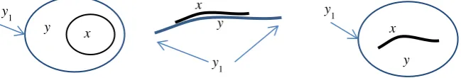
The definition is illustrated in Fig. 3. The feature x is a proper part of y and does not touch the boundary of y. Such a definition of NTPP, though it is different, has exactly the same semantics as the original RCC definition in the case of regions.

Fig. 3. Illustrations of the NTPP definition of RCC*-9. (Note that in the middle illustration, x actually is part of y, but it is drawn alongside it for clarity of illustration; we use the same con-vention in later figures as well).

Fig. 4. Illustration of the O relation.

The new definition for the tangential proper part relation is: Def. 23. TPP(x,y) =def PP(x,y) ∧¬NTPP(x,y)

We can now give a new definition of the overlap relation, which is more restrictive than the corresponding definition of RCC-8:

Def. 24. O(x,y) =def ∃z[NTPP(z,x) ∧NTPP(z,y)] ∧∃t[TPP(t,x) ∧TPP(t,y)] The above definition of overlap expresses the fact that there is a common non-tangential proper part belonging to the two features and a common non-tangential proper part as well. The second part of the rule would not be necessary for regions, but it is necessary for lines (see Fig. 4), otherwise also cases of cross (see later on) would be regarded as overlap.

4_{Since B is a relation rather than a functor in RCC*-9, if y is a closed ring and its boundary}

is empty, it means that there is no value x for which B(x,y) is true. Similarly B(x,y) is never true when y is a point.

x y

y₁ x

y

y₁

x

y y₁

x t _y

z t

z

y t

z x

As in RCC-8, as a refinement of O(x,y), the partially overlap relation corresponds to excluding the inclusion of one feature into the other one:

Def. 25. PO(x,y) =def O(x,y) ∧¬P(x,y) ∧¬P(y,x)

Considering the new domain of spatial features instead of only regions, there are two other kinds of connection that are not included in the overlap definition, namely, the externally connected and the cross relations. We use the following definition for the externally connected relation (which differs from the RCC8 one):

Def. 26. EC(x,y) =def C(x,y) ∧ ¬O(x,y) ∧ ∀z [[P(z,x) ∧ P(z,y)] → [TPP(z,x)∨TPP(z,y)]]

Fig. 5 depicts the EC definition in case of two regions, a region and a line, and two lines. The whole common part z needs to be a tangential proper part of x or y (this is ensured through the universal quantifier ∀z). In the case of a line x and a region y in Fig. 5, the common part z is a tangential proper part of y. Also in the case of the two lines, the common part z is a tangential proper part of y. The EC relation maintains the same semantics as RCC-8 for (2D) regions.

Fig. 5. Illustrations of the EC relation.

Finally, we add the definition of cross, which corresponds to the remaining kind of connection and is not included in the previous ones (see Fig. 6)5:

Def. 27. CR(x,y) =def C(x,y) ∧¬O(x,y) ∧¬EC(x,y)

Fig. 6. Cases of the CR relation.

The inverse relations of the asymmetric part relation and its specializations are de-fined as:

Def. 28. Pi(x,y) =def P(y,x) Def. 29. PPi(x,y) =def PP(y,x) Def. 30. NTPPi(x,y) =def NTPP(y,x) Def. 31. TPPi(x,y) =def TPP(y,x)

5

Note that the cross relation is between a region and a line or a pair of lines; one could also imagine a scenario where two regions “cross” each other (so that they form a kind of “fat cross”; this is not an instance of the cross relation, but just of the PO relation – but see Galton [17] for definitions of relations specialising PO in this way.

x y

z

x

y z

x

y z

x y

For completeness with respect to the original RCC family of calculi, a DR relation (discrete) is defined as:

Def. 32. DR(x,y) =def EC(x,y) ∨DC(x,y)

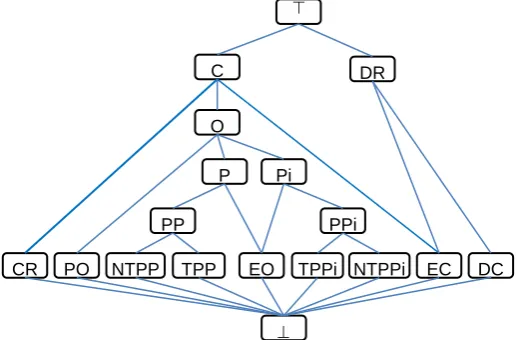
The 9 relations DC, EC, PO, TPP, NTPP, TPPi, NTPPi, EQ, and CR form a provably JEPD set of relations and are the base relations of RCC*-9. A hierarchical implication structure of all the relations defined above is given in Figure 7. To show that Figure 7 correctly reflects the implication hierarchy of the relations is mostly straightforward from the definitions. The only cases which are not trivial are the sub-sumption of O by C, and of P and Pi by O. We also define the JEPD set DC, EC, PO, PP, PPi, EQ, and CR, which we name RCC*-7 and, as we shall see below, corresponds to CBM*.

It is important to stress the fact that the changes we have made to some definitions of RCC-8 to obtain RCC*-9 are alternative definitions of RCC-8 relations to accom-modate multi-type features. There is no change of meaning for these relations if we apply them to (2D) regions. RCC*-9 introduces the new CR relation, which can only hold when one of the entities is a 1D entity.

Fig. 7. The subsumption hierarchy of RCC*-9 relations. The lines indicate semantic inclusion –

i.e., whenever two relations are linked, the lower one implies the upper one.

6

Spatial reasoning

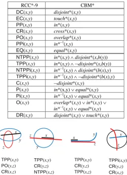
We introduced in Section 4 a modified CBM, called CBM*, and in Section 5 an extension of RCC-8, called RCC*-9. The latter is logically defined in FOPC in terms of a single primitive relation C(x,y) whereas the former’s relations are all taken as primitive and each have their own semantic definitions. It is provable that the two systems can express the same topological relations, as illustrated in Table 1. We can observe a direct correspondence of the base relations of CBM* with the 7 relations of RCC*-7. In CBM*, there are no base relations expressing RCC*-9 relations NTPP

DR C

⊥

Pi

PPi

TPPi NTPPi P

⊥

O

PP

TPP NTPP

PO EQ EC DC

and TPP, which can be expressed by a logical formula involving boundaries of fea-tures.

Table 1. Correspondence between CBM* and RCC*-9.

RCC*-9 CBM*

DC(x,y) disjoint*(x,y)

EC(x,y) touch*(x,y)

PP(x,y) in*(x,y)

CR(x,y) cross*(x,y)

PO(x,y) overlap*(x,y)

PPi(x,y) in*−1(x,y)

EQ(x,y) equal*(x,y)

NTPP(x,y) in*(x,y) ∧ disjoint*(x,b(y)) TPP(x,y) in*(x,y) ∧¬disjoint*(x,b(y)) NTPPi(x,y) in*−1(x,y) ∧ disjoint*(b(x),y) TPPi(x,y) in*−1(x,y) ∧¬disjoint*(b(x),y)

C(x,y) ¬disjoint*(x,y)

P(x,y) in*(x,y) ∨ equal*(x,y)

Pi(x,y) in*−1(x,y) ∨ equal*(x,y)

O(x,y) overlap*(x,y) ∨ in*(x,y) ∨

in*−1(x,y) ∨ equal*(x,y) DR(x,y) disjoint*(x,y) ∨ touch*(x,y)

Fig. 8. Some new cases of composition involving the CR relation.

Given the correspondence between the CBM* and RCC*-9, we proceed to find the composition tables for these calculi. The composition tables contain the basic rules to perform qualitative spatial reasoning with such calculi (see, for example, [9]). Given the relation r1(x,y) and the relation r2(y,z), the composition is the relation r3(x,z). The composition table gives all the possible results of composition for each combination of relations. Such results are expressed as disjunctions of the basic relations. For RCC*-9, the results of compositions are those reported in Table 2. Such a table is a direct extension of the composition table of RCC-8 [11], that is, if we restricted Table

TPP(x,y) PO(y,z) CR(x,z)

z

x

y

TPP(x,y) CR(y,z) NTPP(x,z)

x

y z

TPP(x,y) CR(y,z) TPP(x,z)

x y

z

TPPi(x,y) CR(y,z) CR(x,z)

z y

2 to regions, we would re-obtain the composition table of RCC-8: the CR relation cannot hold between two regions.

In general, the proof of composition tables is difficult, especially when the seman-tics of the calculus depends on higher-order constructs such as sets [24]. There are two aspects to proving that a composition table is correct: (1) showing that each dis-junct in each cell is necessary; (2) showing that there are no missing disdis-junctions. The former is usually achieved by demonstrating (i.e. providing a model such as a figure) of each combination of r1, r2 and a disjunct from r36. Showing that there are no miss-ing disjuncts, given an axiomatic theory of the calculus, can be achieved by provmiss-ing a theorem that r1 and r2 imply r3 for each cell7. If we consider that the RCC*-9 compo-sition table is an extension of the RCC-8 table, one way of finding a proof is ‘by dif-ference’, that is, limiting the analysis to the new cases involving the CR relation only. We found in total 89 new compositions that can be instantiated in R2 involving the CR relation: see Fig. 8 for a sample of them. The fact that no other cases with CR are possible can be proved with a theorem for each entry, but by using redundancy elimi-nation techniques as in [2], the actual number of entries that need to be proved can be reduced significantly. Alternatively, a proof could be developed with a semi-automatic reasoner as proposed in [24]. Besides formal proofs, in future work we also plan to apply heuristics such as in [6], where composition tables can be filled up by running tests on random data sets made up of points, polygons, and polylines.

Table 2. Composition table for RCC*-9.

r2

r1

DC EC PO TPP NTPP TPPi NTPPi EQ CR

DC no info DR, PO,

PP, CR DR, PO, PP, CR DR, PO, PP, CR DR, PO, PP, CR

DC DC DC DR, PO,

PP, CR

EC DR,

PO, PPi, CR DR, PO, TPP, EQ, TPPi, CR DR, PO, PP, CR EC, PO, PP, CR PO, PP, CR

DR DC DC DR, PO,

PP, CR

PO DR,

PO, PPi, CR

DR, PO, PPi, CR

no info PO, PP,

CR PO, PP, CR DR, PO, PPi, CR DR, PO, PPi, CR

PO DR, PO,

PP, PPi, CR

TPP DC DR DR, PO,

PP, CR

PP NTPP DR, PO,

TPP, EQ, TPPi, CR

DR, PO, PPi, CR

TPP DR, PP,

PO, CR

NTPP DC DC DR, PO,

PP, CR

NTPP NTPP DR, PO,

PP, CR

no info NTPP DR, PP,

PO, CR

TPPi DR,

PO, PPi, CR EC, PO, PPi, CR PO, PPi, CR PO, TPP, EQ, TPPi PO, PP, CR

PPi NTPPi TPPi PO, PPi,

CR

NTPPi DR,

PO, PPi, CR PO, PPi, CR PO, PPi, CR PO, PPi, CR

O, CR NTPPi NTPPi NTPPi PO, PPi,

CR

EQ DC EC PO TPP NTPP TPPi NTPPi EQ CR

CR DR,

PO, PPi, CR DR, PO, PPi, CR DR, PO, PP, PPi, CR PP, PO, CR PP, PO, CR DR, PPi, PO, CR DR, PPi, PO, CR

CR no info

6

This is what we actually did to find the RCC*-9 composition table, that is, finding config-urations like those in Fig.8 satisfying each result of the table.

7

From the composition table of RCC*-9, we can infer the composition table of CBM*. First, we need to find an intermediate result: the composition table of RCC*-7. This is just a reduced version of the composition table of RCC*-9 that is obtained by making the union of relations TPP and NTPP and of relations TPPI and NTPPi. From the composition table of RCC*-7 and from the correspondences between CBM* and RCC-7 (Table 1), we can obtain as an almost immediate result the composition table for CBM* (Table 3) by simple renaming of the relations.

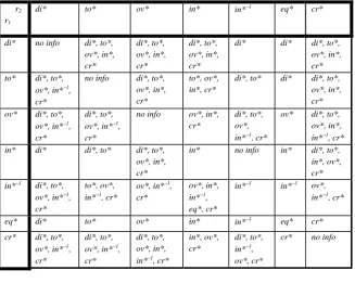
Table 3. Composition table for CBM*. Adopted abbreviations: di=disjoint, to=touch, ov=overlap, eq=equal, cr=cross.

r2

r1

di* to* ov* in* in*−1 eq* cr*

di* no info di*, to*, ov*, in*, cr* di*, to*, ov*, in*, cr* di*, to*, ov*, in*, cr*

di* di* di*, to*, ov*, in*, cr* to* di*, to*,

ov*, in*−1, cr*

no info di*, to*, ov*, in*, cr*

to*, ov*, in*, cr*

di*, to* di* di*, to*, ov*, in*, cr* ov* di*, to*,

ov*, in*−1, cr*

di*, to*, ov*, in*−1, cr*

no info ov*, in*, cr*

di*, to*, ov*, in*−1, cr*

ov* di*, to*, ov*, in*, in*−1, cr* in* di* di*, to* di*, to*,

ov*, in*, cr*

in* no info in* di*, to*, in*, ov*, cr* in*−1 di*, to*,

ov*, in*−1, cr*

to*, ov*, in*−1, cr*

ov*, in*−1, cr*

ov*, in*, in*−1, eq*, cr*

in*−1 in*−1 ov*, in*−1, cr*

eq* di* to* ov* in* in*−1 eq* cr*

cr* di*, to*, ov*, in*−1, cr*

di*, to*, ov*, in*−1, cr*

di*, to*, ov*, in*, in*−1, cr*

in*, ov*, cr*

di*, to*, in*−1, ov*, cr*

cr* no info

7

Comparison with 9-intersection

be-tween CBM* and 9IM. The equivalent expressions of 9IM can be easily inferred from CBM* definitions.

Table 4. Correspondence between CBM* relations and 9IM relations.

CBM* 9IM

disjoint*(x,y) Relate(x,y,"FF*FF****") touch*(x,y) Relate(x,y,"FTT***T**")∨

Relate(x,y,"F*TT**T**")∨ Relate(x,y,"F*T*T*T**") in*(x,y) Relate(x,y,"**F**F***")∧

¬Relate(x,y,"TFFFTFFFT") cross*(x,y) Relate(x,y,"T**FF****")∨

Relate(x,y,"TF**F****") overlap*(x,y) Relate(x,y,"TTTT**T**")∨

Relate(x,y,"T*T*T*T**") in*−1(x,y) Relate(x,y,"******FF*")∧

¬Relate(x,y,"TFFFTFFFT") equal*(x,y) Relate(x,y,"TFFFTFFFT")

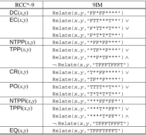
Table 5. Correspondence between RCC*-9 and 9IM.

RCC*-9 9IM

DC(x,y) Relate(x,y,"FF*FF****")

EC(x,y) Relate(x,y,"FTT***T**")∨

Relate(x,y,"F*TT**T**")∨ Relate(x,y,"F*T*T*T**")

NTPP(x,y) Relate(x,y,"*FF*FF***")

TPP(x,y) Relate(x,y,"*TF**F***")∨

Relate(x,y,"**F*TF***")∧

¬Relate(x,y,"TFFFTFFFT") CR(x,y) Relate(x,y,"T**FF****")∨

Relate(x,y,"TF**F****") PO(x,y) Relate(x,y,"TTTT**T**")∨

Relate(x,y,"T*T*T*T**") NTPPi(x,y) Relate(x,y,"***FF*FF*") TPPi(x,y) Relate(x,y,"***T**FF*")∨

Relate(x,y,"****T*FF*")∧

¬Relate(x,y,"TFFFTFFFT")

EQ(x,y) Relate(x,y,"TFFFTFFFT")

expressive DE+9IM. The CBM relations needed the dimension to find equivalent expressions in the DE+9IM matrices, being 9IM matrix alone not sufficient. In [3], it was proved that CBM is equivalent to DE+9IM in terms of the number of topological configurations that the models are able to distinguish. Though it is out of the scope of this paper, it is provable that CBM* is equivalent to 9IM in terms of number of topo-logical configurations. In this sense, CBM* can be considered weaker than CBM because CBM* does not include the possibility of checking the dimension of intersec-tions. Of course, this is not a real weakness of CBM* since an operator to check di-mension could be easily added to the calculus to recuperate the ability of checking set dimension. Given the correspondence between CBM* and RCC*-9 (Table 1), we can express RCC*-9 relations in terms of 9IM matrices by using Table 4 to obtain Table 5.

8

Conclusions and further work

An extension towards multidimensional mereotopology [18] has been advocated for a long time. RCC*-9 is our contribution to address this issue. We defined RCC*-9 by modifying the definition of the basic relations of RCC-8 and adding two new rela-tions, namely, a new primitive B(x,y) to express that x is boundary of y and CR(x,y) for the defined cross relation. The variables of RCC*-9 no longer range just over regions, but features (or sets of features) of dimension 2, 1, or 0, embedded in R2. These changes extend rather than change8 the semantics of RCC-8, since if we con-sider only regions, then RCC*-9 collapses to RCC-8. The composition table of RCC*-9 with respect to the composition table of RCC-8 presents the relation CR as an additional possible result of composition, but it does not affect the already present results – i.e. each entry in the composition table for RCC*-9 is either the same, or a superset of the corresponding RCC-8 composition table entry (except for the rows and columns labelled by CR, which are new).

In this paper, we also introduced the CBM*, a modified version of CBM where we lose the possibility of distinguishing the dimension of set intersections. CBM* defini-tions do not depend on the type of features, e.g., a cross between two lines has the same definition of the cross between a line and a region. With the new definitions, it is possible to obtain a single composition table for all features.

Finally, we provided the usual basis for a reasoning system for a qualitative calcu-lus, i.e. a composition table, for the new calculi, extending the earlier composition tables from simple regions to the case of generic spatial features. Another interesting aspect that we discussed is how to find equivalent expressions of both calculi in terms of 9IM, which is essential to enabling a straightforward implementation in OGC-compliant systems.

Further work is needed to provide a formal proof of the correctness of the composi-tion tables. Another issue that is not covered in this paper is the study of the cognitive

8

Strictly, it only extends RCC8 if we consider the 2D interpretation of RCC8: RCC8 can

be interpreted in any dimension ≥ 2; in principle the definitions here may apply to regions of

adequacy of the group of relations inside CBM* and RCC*-9 models. It would be interesting to find out the differences in subjective perceptions especially of the pre-vious CBM calculus versus the new CBM* calculus. Finally, an assessment of how the calculi behave for complex features and for higher dimensional spaces remains to be done.

Acknowledgements. Authors wish to express their gratitude to the referees for their useful suggestions and to Paolo Fogliaroni for his comments to a previous version of the manuscript. The financial support of EU projects RACE (FP7-ICT-287752) and STRANDS (FP7-ICT-600623) is gratefully acknowledged.

References

[1] W. G. Aref and H. Samet, "Optimization Strategies for Spatial Query Processing," in 17th International Conference on Very Large Databases, Barcelona, Spain, 1991, pp. 81-90.

[2] B. Bennett, Logical Representations for Automated Reasoning about Spatial Relationships. Ph.D. Thesis, School of Computer Studies, University of Leeds, 1997.

[3] E. Clementini and P. Di Felice, "A Comparison of Methods for Representing Topological Relationships," Information Sciences, vol. 3, pp. 149-178, 1995. [4] E. Clementini and P. Di Felice, "A Model for Representing Topological

Relationships Between Complex Geometric Features in Spatial Databases," Information Sciences, vol. 90, pp. 121-136, 1996.

[5] E. Clementini, P. Di Felice, and P. van Oosterom, "A Small Set of Formal Topological Relationships Suitable for End-User Interaction," in Advances in Spatial Databases - Third International Symposium, SSD '93. vol. 692, D. Abel and B. C. Ooi, Eds. Berlin: Springer-Verlag, 1993, pp. 277-295. [6] E. Clementini, S. Skiadopoulos, R. Billen, and F. Tarquini, "A reasoning

system of ternary projective relations," IEEE Transactions on Knowledge and Data Engineering, vol. 22, pp. 161-178, 2010.

[7] E. F. Codd, "A relational model for large shared data banks,"

Communications of the ACM, vol. 13, pp. 377-387, 1970.

[8] A. G. Cohn, B. Bennett, J. Gooday, and N. Gotts, "Qualitative Spatial Representation and Reasoning with the Region Connection Calculus," GeoInformatica, vol. 1, pp. 275-316, 1997.

[9] A. G. Cohn and J. Renz, "Qualitative Spatial Representation and Reasoning," in Handbook of Knowledge Representation, 1, F. v. Harmelen, V. Lifschitz, and B. Porter, Eds.: Elsevier, 2007, pp. 551-596.

[10] A. G. Cohn and A. C. Varzi, "Mereotopological connection," Journal of Philosophical Logic, vol. 32, pp. 357-390, 2003.

[12] M. J. Egenhofer, "Deriving the composition of binary topological relations," Journal of Visual Languages and Computing, vol. 5, pp. 133-149, 1994. [13] M. J. Egenhofer, E. Clementini, and P. Di Felice, "Topological relations

between regions with holes," International Journal of Geographical Information Systems, vol. 8, pp. 129-142, 1994.

[14] M. J. Egenhofer and R. D. Franzosa, "Point-Set Topological Spatial Relations," International Journal of Geographical Information Systems, vol. 5, pp. 161-174, 1991.

[15] M. J. Egenhofer and J. R. Herring, "Categorizing Binary Topological Relationships Between Regions, Lines, and Points in Geographic Databases," Department of Surveying Engineering, University of Maine, Orono, ME Technical Report, 1990.

[16] N. Gabrielli, Investigation of the Tradeoff between Expressiveness and Complexity in Description Logics with Spatial Operators. Ph.D. Thesis: University of Verona, 2009.

[17] A. Galton, "Modes of overlap," Journal of Visual Languages and Computing, vol. 9, pp. 61-79, 1998.

[18] A. Galton, "Multidimensional Mereotopology," in Proceedings of the Ninth International Conference on Principles of Knowledge Representation and Reasoning (KR2004), D. Dubois, C. Welty, and M.-A. Williams, Eds. Whistler, BC, Canada, June 2-5, 2004: American Association for Artificial Intelligence, 2004, pp. 45-54.

[19] A. P. Galton, "Taking dimension seriously in qualitative spatial reasoning," in Proceedings of the Twelfth European Conference on Artificial Intelligence (ECAI’96), Budapest, Hungary, 11th - 16th Aug 1996, 1996.

[20] A. Gerevini and J. Renz, "Combining topological and size information for spatial reasoning," Artificial Intelligence, vol. 137, pp. 1-42, 2002.

[21] N. M. Gotts, "Formalizing Commonsense Topology: The INCH Calculus. pp.," in Proceedings of the Fourth International Symposium on Artificial Intelligence and Mathematics, 1996.

[22] A. Isli, L. Museros Cabedo, T. Barkowsky, and R. Moratz, "A Topological Calculus for Cartographic Entities " in Spatial Cognition II vol. LNCS 1849 Berlin: Springer, 2000, pp. 225-238.

[23] OGC Open Geospatial Consortium Inc., "OpenGIS Simple Features

Implementation Specification for SQL." vol. OGC 99-049, 1999.