Dynamic Model Generation and Classification of Network Attacks

(1)

Theses Thesis/Dissertation Collections

5-2017

Dynamic Model Generation and Classification of

Network Attacks

Jacob D. Saxton

jds8588@rit.edu

Follow this and additional works at:http://scholarworks.rit.edu/theses

This Thesis is brought to you for free and open access by the Thesis/Dissertation Collections at RIT Scholar Works. It has been accepted for inclusion in Theses by an authorized administrator of RIT Scholar Works. For more information, please contactritscholarworks@rit.edu.

Recommended Citation

(2)

Dynamic Model Generation and Classification of

Network Attacks

(3)

Jacob D. Saxton May 2017

A Thesis Submitted in Partial Fulfillment

of the Requirements for the Degree of Master of Science

in

Computer Engineering

(4)

Dynamic Model Generation and Classification of

Network Attacks

Jacob D. Saxton

Committee Approval:

Dr. Shanchieh Jay Yang Advisor Date

Professor

Dr. Andres Kwasinski Date

Associate Professor

Dr. Andreas Savakis Date

(5)

I would like to thank my thesis committee for their time and help in completing my

thesis. I would especially like to thank my advisor, Dr. Shanchieh Jay Yang for his

continued assistance and the eﬀort he put into helping me whenever it was needed.

I would also like to thank my friends and family for their support throughout my

(6)

This thesis is dedicated to my grandfather, Thomas Damon, for his continual

support in my education. He was the first person to get me interested in science and

(7)

When attempting to read malicious network traﬃc, security analysts are challenged to

determine what attacks are happening in the network at any given time. This need to

analyze data and attempt to classify the data requires a large amount of manual time

and knowledge to be successful. It can also be diﬃcult for the analysts to determine

new attacks if the data is unlike anything they have seen before. Because of the

ever-changing nature of cyber-attacks, a need exists for an automated system that can

read network traﬃc and determine the types of attacks present in a network. Many

existing works for classification of network attacks exist and contain a very similar

fundamental problem. This problem is the need either for labeled data, or batches of

data. Real network traﬃc does not contain labels for attack types and is streaming

packet by packet. This work proposes a system that reads in streaming malicious

network data and classifies the data into attack models while dynamically generating

and reevaluating attack models when needed.

This research develops a system that contains three major components. The first is a

dynamic Bayesian classifier that utilizes Bayes’ Theorem to classify the data into the

proper attack models using dynamic priors and novel likelihood functions. The second

component is the dynamic model generator. This component utilizes the concept of

a cluster validity index to determine the proper time to generate new models. The

third component is a model shuﬄer. This component redistributes misclassified data

into attack models that more closely fit the behaviors of the data. Malicious packet

captures obtained from two network attack and defense competitions are used to

demonstrate the ability of the system to classify data, successfully and reasonably

(8)

List of Figures

3.1 Abstraction Levels . . . 12

3.2 Classification and Model Generation Overview . . . 13

3.3 Example Attack Social Graph . . . 15

3.4 Example Model Feature Histograms . . . 15

3.5 Model Generation Decision Flowchart . . . 22

3.6 System Flow . . . 27

4.1 CPTC2 data with shuﬄe parametersIT = 0.75 and NI = 500 . . . . 32

4.2 CPTC2 data with shuﬄe parametersIT = 0.75 and NI = 1500 . . . . 32

4.3 Uniform Prior Over Iterations . . . 33

4.4 Edge Based Prior Over Iterations . . . 34

4.5 Times Series Based Prior Over Iterations . . . 34

4.6 100 Iterations Edge Based Prior . . . 35

4.7 100 Iterations Time Series Based Prior . . . 35

4.8 Index Using Uniform Prior . . . 36

4.9 Index Using Edge Based Prior . . . 36

4.10 Index Using Time Series Based Prior . . . 37

4.11 Model 0 Features . . . 38

4.14 New Model Features . . . 40

4.15 Index Over Iterations with Shuﬄing . . . 41

4.16 Index Over Iterations with no Shuﬄing . . . 41

4.17 Index at Shuﬄing . . . 42

4.18 Model 0 Features Before Shuﬄing . . . 42

4.25 Model 0 Features After Shuﬄing . . . 44

(11)

(12)

List of Tables

4.1 Performance Metrics with Varying Shuﬄe Trigger Parameters . . . . 31

4.2 Index Value at Iteration 1,501 Using Diﬀerent Priors . . . 37

4.3 Comparison of Priors Using Performance Metrics . . . 37

4.4 Posteriors of New Edge Belonging to Existing Models . . . 39

4.5 Index Comparison for Model Generation . . . 40

(13)

Introduction

In the field of cyber security, the information gained from network attacks

continu-ously increases. As new vulnerabilities are discovered within a network and as the

tools used by attackers become more sophisticated, the abilities and methods of the

people attacking the network evolve as well. These attackers are also continuously

changing and developing their tactics for attacking a network. Many current attackers

use simple techniques that are often more diﬃcult to detect. Advanced techniques

are rare and are used sparingly [19]. Because of this, if new attacks are used against

a network that the analyst is not familiar with, the attack could remain undetected

until severe damage is done to the network. Because of these developments, security

analysts face diﬃculties in determining the types of attacks being used against their

network in a reasonable time period. The quick evolution of cyber-attacks, presents

a need for a robust system that can read malicious network activity and either

clas-sify them into existing attack models, or create a new model based on the observed

activity. The main challenges in developing such a system is that the large amount

of traﬃc entering a network is unlabeled for attack types and streaming.

While security analysis methods exist to classify attack types, they contain two

ma-jor flaws. Current methods require some ground truth knowledge of attack types in

order to categorize diﬀerent attacks. This requirement of ground truth knowledge

(14)

CHAPTER 1. INTRODUCTION

Many current methods also analyze the data in large batches and does not classify the

traﬃc as it enters the system. This limits the ability of security analysts to quickly

and eﬀectively determine ongoing attacks within the network and could prevent them

from taking the necessary measures to stop the attacker and preserve their important

information. NASS, a system developed and described by Strapp [16] attempts to

resolve these problems. NASS uses dynamic Bayesian analysis to classify incoming

malicious network traﬃc data into attack models, either by classifying the data into

the model that most closely matches the data, or by creating a new model that better

fits the new data.

This work presents a system to solve the problem of classifying streaming unlabeled

malicious network traﬃc. Malicious network attacks as referred to in this work are

not any specific malware or exploits. Instead, malicious network attacks describes

the presence of malicious activities occurring between IP Address pairs on the

net-work. These activities are then evaluated and classified based on the specific features

(ports, protocols, etc.) observed in the traﬃc between the IP Addresses. The main

components of the system are outlined below:

• A dynamic Bayesian classifier including a Bayesian prior probability calculation

based on the time series analysis of the data being input into the system

• A new way of dynamically creating attack models using graphical properties of

an Attack Social Graph as opposed to a simple threshold

• A method to measure the quality of the attack models to trigger shuﬄing of

the data inside the models to ensure the accuracy of the classification

This work develops a system that is able to accurately classify streaming malicious

network traﬃc into diﬀerent attack models based on the specific features of the

ob-servables. The novel contributions include:

(15)

truth knowledge of how many models, or the features of any existing models, the

ability to dynamically generate models based on the observed network traﬃc is vital

for accurate classification. This work presents a way to determine when to generate

models using a cluster validity index to determine the quality of the classifications.

Model Shuﬄing Because of the nature of the streaming data, as classification is

done it is possible that the classification is not fully optimal as misclassification may

occur. Because of this possibility, a way to shuﬄe data into the existing models to

change optimize the classification was developed.

Dynamic Bayesian Prior In using Bayes’ Theorem for the classification of the

network traﬃc, an informative Bayesian prior is important to allow for proper

classi-fication. Because of the lack of ground truth knowledge in the data, a true Bayesian

prior does not exist. For this reason, a dynamic Bayesian prior was developed to

describe the probability of the model adding new edges based on the information

(16)

Chapter 2 Related Works

While works exist to solve the problems of classifying network attacks, classifying

unlabeled data, and classifying streaming data the three problems are rarely tackled

together. The problem to be solved in this work is the ability to classify unlabeled,

streaming, network attack data which combines these three concepts. The method

presented in this work is that of a dynamic classifier that is constantly assessed

with a cluster validity index. Sections 2.1 and 2.2 explore works in network attack

classification. Section 2.1 discusses general methods for recognizing network attacks

while Section 2.2 expands on the concept of using a social graph to model network

attacks and further explores the NASS framework. Section 2.3 explores clustering,

a common method of classifying unlabeled data, along with the general concept of

cluster validity indexes. Section 2.4 discusses works that exist to classify streaming

data.

2.1 Network Attack Recognition

The need to recognize network attacks is already a well known problem. Early works

created taxonomies of network attacks. These taxonomies attempt to collect

infor-mation on known attack strategies and compile a list so that a network attack can

be recognized after it has occurred. Two popular and widely accepted taxonomies

(17)

Lough’s taxonomy, VERDICT, written in 2001. Howard’s taxonomy groups attacks

based on the motivations and objectives of the attacker, as well as the results of the

attack while VERDICT provides a characteristic based attack taxonomy that

de-scribes how the attack happened, for example, if insuﬃcient validation requirements

exist for access to the system.

As network attacks have grown more sophisticated, the tools used to model them

have become more sophisticated as well. Al-Mohannadi et al. [2] provide an overview

of some of the more popular methods of modeling network attacks. Attack graphs

are the most commonly used method of attack modeling in computer science because

it allows for searchability within a computer system or an algorithm. Attack graphs

are used to identify the vulnerabilities of a system, how attacks can happen on the

network, and a set of actions that can be taken to prevent an attacker. The purpose

of an attack graph is to identify any and all potential attacks on the network. The

kill chain model is the model used by the United States Department of Defense both

in modeling cyber attacks, as well as attacks on the battlefield. A kill chain describes

how an attack is performed as a chain of actions from reconnaissance to action on

the objectives. A Capability-Opportunity-Intent (COI) Model is a method of attack

modeling that is used for intrusion analysis and represents an attacker’s motivation

rather than their attack path. When using this model, the attack is described by the

personality and capabilities of the attacker, the infrastructure of the network being

attacked, and the defendability of the attacker [15].

Building on the attack graph model, Aguessy et al. [1] presented a Bayesian Attack

Model (BAM) for dynamic risk assessment. This work combines the ideas of a

topo-logical attack graph and a Bayesian network in order to probabilistically represent

all possible attacks in an information system. The attack graph is based on a

di-rected graph where the nodes, the hosts and IP addresses, are topological assets and

(18)

CHAPTER 2. RELATED WORKS

graph developed is an extension of the attack graph based on a Bayesian network

where each node represents a host in a specific system state and the edges represent

possible exploits between a source host and a target host. The BAM uses a

modi-fied Bayesian attack graph with topological nodes that are assets of the information

system and edges that are attack steps. These edges represent an attack that allows

the attacker to move from one topological node to the next and describes how the

attacker moves between the nodes, for example through an exploitation of a

vulnera-bility or a theft of credentials. The nodes are also associated with a random variable

that describes either the state of the node being compromised or the success of an

at-tack step. Through this BAM, all possible atat-tacks on a network are probabilistically

mapped out so that an analyst can see where the major vulnerabilities in the system

are.

More recent works regarding the recognition of network attacks have mainly been

done in the area of intrusion detection systems. Many of these types of systems exist

and their purpose is to detect an intruder in the network so that preventative

mea-sures can be taken to either stop the attacker from progressing through the network

or prevent an intrusion from the same entry point from happening again. Two such

examples are the works by Subba, Biswas, & Karmakar [18] and Haddadi, Khanchi,

Shetabi, & Derhami [7].

While intrusion detection systems are becoming more sophisticated and more

accu-rate they continue to have two major drawbacks. The first is that intrusion detection

systems often raise large numbers of false positives in the data. The second is that

any intrusions detected must be evaluated by a security professional to determine the

proper course of action to be taken. One way to solve these problems is to integrate an

attack classifier into the intrusion detection system as explored in the works of Luo,

Wen, & Xian [12] and Bolzoni, Etalle, & Hartel [3]. Luo et al. use a Hidden Markov

(19)

Bolzoni et al. use Support Vector Machines (SVM) and the RIPPER rule learner

comparing byte sequences from alert payloads. The major drawback of comparing

byte sequences for classification is that attacks that do not involve a payload, i.e.

port scan or DDOS, cannot be classified.

The problem with current attack classification systems is that they require training

in order to perform the classification. Because of this, new or rare attacks become

very diﬃcult to classify. In order to mitigate this risk, Yang, Du, Holsopple, & Sudit

[21] propose a semi-supervised system to classify network attack behaviors in asset

centric attack models. These asset centric attack models group collective evidences

and create models based on these groups. Evidences that have similar features are

classified into the same attack model using a Bayesian classifier to create an attack

behavior model, which is a collection of feature probability distributions.

2.2 Attack Social Graph and the NASS Framework

The concept of using a social graph to describe network attacks is described by Du &

Yang [6]. This work describes the use of an Attack Social Graph (ASG) to describe

attacks on a network. In this work, features are extracted from this graph and used

to determine any patterns that can be seen in the data. Principle component analysis

(PCA) is used to reduce the feature space and hierarchical clustering is used to group

sources of attacks that demonstrate similar behaviors.

The work by Du & Yang was then expanded upon by Strapp [16] in his creation of the

NASS framework. In his work, Strapp built upon the concepts set forth by Du & Yang

by using dynamic Bayesian Analysis to determine the probability of a new data point

of malicious network traﬃc belonging to an attack model. He abstracts all individual

observables in a data set into edges on the ASG with the source and destination IP

Addresses being the nodes. These edges are then used to create dynamic models

(20)

and inherits its features from the edges that are classified into it. Iterative Bayesian

Analysis in this work uses Bayes’ Theorem to classify attack behaviors into attack

models. If the behavior does not closely match any of the existing models, a new

model will be created using that behavior as the basis for the new model’s features.

As edges are classified into the models, the features of the models are modified to

include the features on the edges that are classified into the model. Because of this, the

models change as new edges are classified into them. This can lead to major problems

in the classification because the edges are also changing when new observables are

added to them. Because the edges are classified upon creation, as they change with

new observables being added, the model that the edge is initially classified into may

not be the best fit for that edge as time goes on. For this reason, a way is needed

to periodically change which model an edge is classified to if a better fit becomes

apparent.

Two other challenges that exist in the NASS framework are the creation of a new

model, and the Bayesian prior probability. In the original NASS framework, a generic

model was used to determine when to create a new model. The generic model was

a static model that contained features that was intended to fit all behaviors with a

modest probability. Whenever a new edge was to be classified, the probability of

it belonging to any existing model would be determined. If the edge had a higher

probability of belonging to the generic model then any of the other models, a new

model would be created for the edge. The problem raised when using the generic

model is that even if a new behavior enters the system, if it has a higher probability

of belonging to an existing model then the generic model, a new model will not be

made and the edge will be classified to the existing model. The generic model would

also have to be continuously updated so that it would continue to match all behaviors

with a modest probability.

(21)

ASG to determine the probability of an attack model before considering the features in

the observables. The prior probability is calculated using the idea of graph eﬃciency

and is determined by how centralized the models in the ASG are by attempting to

infer collaborating groups of IP Addresses at a target. While this is a valid strategy

and often times collaborating groups of IP Addresses will exist, at the core this prior

is not strictly ”Bayesian”. A Bayesian prior probability, by definition, should give

an idea of which model the edge should be classified without being influenced by the

features on the edge or models. Using graphical properties of the models breaks this

definition.

2.3 Clustering

Clustering is a very popular method of classifying any sort of data and can be used

to classify data without any ground truth knowledge. However, clustering has two

major drawbacks. The first is that clustering requires knowledge of all data points at

the same time for the clustering to be successful. The other is that it can be quite

diﬃcult to determine how successful a clustering has been without expert knowledge

of the dataset or ground truth labels. In order to solve this second problem, the works

of both Wang, Wang, & Peng [20] and Kovacs, Legancy, & Babos [10] explore the

use of cluster validation indexes to determine the quality of a clustering algorithm.

These validation indexes take into account the separation between clusters along with

the closeness of data points within the same cluster to determine if the clustering is

reasonable. These cluster validation indexes are used to determine the quality of a

clustering algorithm using the graphical properties of the clusters. This also translates

into a quality assessment of the classification being done by the algorithm. This work

uses the cluster validation index and to constantly analyze the quality of classification

in order to assist in determining when to dynamically generate new models and when

(22)

2.4 Classification of Streaming Data

Classification of streaming data as opposed to data sets is a growing problem but one

that is still relatively new. Streaming data is defined as data that enters the system

one observable at a time. One common method for the classification of streaming

data is to use ensemble algorithms such as those described by Street & Kim [17]

and Kuncheva [11]. These ensemble algorithms are built by combining the results of

multiple types of classifiers on a subset of the data stream. The final classification is

then determined by voting. Another common practice for classifying streaming data

is to store data points in memory until a small subset is gathered and then performing

the classification on these data chunks. The classification can either be done using

an ensemble algorithm as done by Street & Kim and Kuncheva, or by clustering

as described by O’Callaghan [14]. This work addresses the common problems in

streaming data classification by classifying unlabeled observables one at a time as

they enter the system as opposed to holding the data in memory and classifying

subsets of the data stream. This work also classifies using a Bayesian classifier as

(23)

Methodology

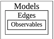
The framework developed does not classify observables themselves. Instead, the

ob-servables, in this case malicious network packet capture data, are abstracted to edges

in the Attack Social Graph (ASG). The edges in the ASG are made up of a collection

of all network traﬃc between two IP Addresses acting as nodes. As observables enter

the system and are added to the edges, the features of the observable are added to the

feature histograms on the edge. These edges are then classified into the attack models

that characterize diﬀerent attack behaviors. The models represent a collective

behav-ior of malicious attributes from all edges classified to the model. The assumption

driving this abstraction is that activity over a single edge between two IP Addresses

in a short period of time will be indicative of one single behavior. As edges are

clas-sified to models, the feature histograms of the edges are added to those of the model.

This abstraction can be seen in Figure 3.1.

[image:23.612.269.380.574.654.2]

The framework developed contains three separate parts that work together to solve

Figure 3.1: Abstraction Levels

(24)

CHAPTER 3. METHODOLOGY

Bayesian classifier. The Bayesian classifier is the main portion of the system and is

the block used to classify the network attack data into attack models. The second

block is a dynamic model generator. The notion of dynamic model generation is a

response to the data containing no ground truth of how many or what types of models

exist. The dynamic model generation is used to determine at what point a new

at-tack behavior becomes present in the data and creates new atat-tack models from these

behaviors. The third block is a model shuﬄing block. In classifying streaming

unla-beled data, the models created are ever changing. For this reason, it is reasonable to

assume that, over time, some of the attack data will be classified into models that no

longer represent the behavior of the data. For this reason, the model shuﬄing block

was developed to periodically reassess the classification and, if needed, reclassify the

data into diﬀerent attack models. These three blocks are shown in Figure 3.2.

The first portion of the framework is the Bayesian classifier. This classifier

con-Figure 3.2: Classification and Model Generation Overview

tains the calculations for the likelihood and the Bayesian prior, and combines them

to calculate the Bayesian posterior used for classification. This portion is described

in Section 3.1.

The second block is the dynamic model generation. This block uses the concept of

a cluster validity index to generate cyber attack models. This block is described in

Section 3.2.

The third block is the model shuﬄing block. Contained in this portion is the

trigger-ing, edge reclassification, and stopping criteria to shuﬄe edges within existing models.

(25)

Section 3.4 describes how the three blocks work together to complete the dynamic

model generation and classification process.

3.1 Dynamic Bayesian Classifier

The dynamic classifier developed builds on the NASS framework developed by Strapp.

This classifier assumes that the framework contains reasonable features for the

ob-servables being classified and proper Bayesian likelihood probability calculations for

these features. At the time of this work, the features existent in the framework are:

• Network Protocol

• Source Port

• Destination Port

• Source Port Transition Matrix

• Destination Port Transition Matrix

The source and destination port transition matrices are the probability that an

at-tacker will change from using one source or destination port to using another.

This dynamic classifier was developed to solve the problem of classifying streaming

attack data. As such, the classifier assumes that all incoming data is analyzed

inde-pendently and in a set order. The classifier utilizes Bayes’ Theorem shown in (3.1).

Section 3.1.1 describes the equation used to calculate the likelihood and Section 3.1.2

describes the equations used to determine the prior.

P(Ω|x)

P rior z }| {

P(Ω)

Likelihood z }| {

P(x|Ω)

∑

Ωi

P(Ωi)P(x|Ωi)

(3.1)

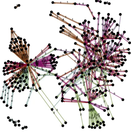
An example of the ASG can is shown in Figure 3.3. In this graph, the black nodes

(26)

one IP Address to the other. The colors of the edges represent to which model the

edge has been classified.

The models being created are non-parameterized and are expressed as a collection

Figure 3.3: Example Attack Social Graph

of distributions of each attribute of malicious activity. An example of the feature

histograms present on a model can be seen in Figure 3.4. This example contains

three separate feature histograms describing the Destination Port, Source Port, and

Network Protocol features. Each bar on the histogram represents the count for an

individual value for that feature (ex. Destination Port = 22).

[image:26.612.221.431.149.361.2]

When a new observable is analyzed, it is added to the edge on the ASG between

Figure 3.4: Example Model Feature Histograms

(27)

created and added to the ASG. At the point of creation, the edge is classified to

either an existing attack model in the system, or is used to generate a new attack

model. Section 3.2 details the dynamic model generation process. If a new model is

not created, the edge is classified to the maximum a posteriori model. Algorithm 1

describes the process of analyzing an observable in the system.

Algorithm 1 Add Observable

1: function addObservable(p)

2: if p.sourceIP not exist in ASG then 3: ASG.createN ode(p.sourceIP)

4: if p.destIP not exist in ASG then 5: ASG.createN ode(p.destIP)

6: if edge between p.sourceIP and p.destIP not exist in ASGthen

7: e=ASG.createEdge(p.sourceIP, p.destIP)

8: for model m in ASGdo

9: e.calculateLikelihood(m)

10: e.calculateP osterior(m)

11: classif y(e)

12: else

13: e=ASG.getEdge(p.sourceIP, p.destIP) 14: e.add(p)

15: ASG.updateP riors()

17: e.calculateLikelihood(m)

18: mod=e.getM odel()

19: for edge ed inASG do

20: ed.calculateLikelihood(mod)

21: for model m inASG do

22: ed.calculateP osterior(m)

3.1.1 Likelihood

The likelihood calculation is done by determining the likelihood of a single model

feature histogram producing an edge feature histogram using the equation shown in

(3.2) where pi is the probability of a feature in a model (ex. if a model contains

three packets with destination port 66 out of ten total packets, pi = 0.3) andei is the

(28)

with destination port 66, ei = 4).

l=∏pei

i ×

(∑_∏ei)! ei!

(3.2)

Then, Shannon entropy is used to determine the stochastic or deterministic nature

of the feature. If many diﬀerent feature values are seen on the same edge with a

similar number of occurrences, the edge displays a more stochastic behavior for that

particular feature. This entropy is then combined with the likelihood from (3.2) as

shown in (3.3) whereE is the entropy value.

P(x|Ω)f = (1−E)l+E (3.3)

These likelihood with entropy values are then multiplied together for all features

present on the edge being classified as shown in (3.4). This multiplication assumes

independence of the individual features.

P(x|Ω) =∏

f

P(x|Ω)f (3.4)

3.1.2 Dynamic Bayesian Prior

In order to use Bayesian classification, it is important to have a Bayesian prior that

defines the probability of an edge belonging to an attack model without taking into

account the features in the model or in the edge. In order to obtain an informative

prior without any ground truth knowledge, the concept of a dynamic Bayesian prior

was explored. A dynamic prior is one that changes with the information available in

the system. Three diﬀerent priors were explored. Section 3.1.2.1 describes a uniform

prior based on the number of models that exist in the system. Section 3.1.2.2 describes

a prior based on the number of edges in each model in the system. Section 3.1.2.3

(29)

based on trends in the data.

3.1.2.1 Uniform

A uniform prior is the most basic and uninformative of the three priors. The uniform

prior is one that simply states that all models are equally likely to have new edges

classified into them. The value for the prior in this case is simply the inverse of the

number of models as shown in (3.5) where N is the number of models that exist in

the system.

P(Ω) = 1

N (3.5)

3.1.2.2 Edge Based

An edge based prior is more informative than the uniform. This prior states that the

more edges a model contains, the more likely it is that new edges will be classified into

that model. This is similar to the standard Bayesian prior that provides information

based on the number of samples in each class. The value for this prior is obtained as

shown in (3.6) wherenΩ is the number of edges classified in model Ω.

P(Ω) = ∑nΩ

inΩi

(3.6)

3.1.2.3 Time Series Based

The time series based prior is the most informative and novel of the three priors

explored. This prior attempts to predict the number of edges classified into each

model based on the recent trends in the data. This prior states that more recently

active models will have a higher probability of gaining new edges. This prior was

developed using the concept of Holt-Winters double exponential smoothing. Double

exponential smoothing is often used in conjunction with data that shows a trend in

(30)

the prediction for t ≥ 2 are shown in (3.7) and (3.8), where α and β are smoothing

parameters.

st=αxt+ (1−α)(st−1+bt−1) (3.7)

bt =β(st−st−1) + (1−β)bt−1 (3.8)

Fort = 1, the equations are shown in (3.9) and (3.10).

s1 =x1 (3.9)

b1 =x1−x0 (3.10)

In order to predict a value beyond time t, the equation shown in (3.11) is used.

Ft+m =st+mbt (3.11)

In the context of the Bayesian classifier, the value ofFt+m is modified in order to give

a valid probability value for the prior as shown in (3.12).

P(Ω) = ∑Ft+1Ω

ΩiFt+1Ωi

(3.12)

To use this prior in the classifier, the value for xt must be defined. In Holt-Winters

double exponential smoothing, xt is defined as the actual value of the data that is

being forecast at time t. Using this definition, it can be determined that, in order

for the prior to follow the definition of a traditional Bayesian prior, the value of xt

should be the same as the component being classified. Because of this, the value of

(31)

3.2 Dynamic Model Generation

As is the case with any sort of classification without ground truth knowledge of

the dataset, the problem arises of how to determine which models to create. If the

data was all to be collected and then analyzed, clustering algorithms could be used.

However, due to the streaming nature of the data, the models must be dynamically

created in real time as the data is being read into the system. This raises the challenge

of knowing at what point a new model must be created. The hypothesis discussed

in this section is to use the concept of a cluster validity index to measure the quality

of the ASG to aid in determining when these models should be created. Subsection

3.2.1 will discuss the concept of the cluster validity index and Subsection 3.2.2 will

describe how this concept can be used for dynamic model generation

3.2.1 Cluster Validity Index

Cluster validity indexes are used to measure the quality of a clustering algorithm.

There exist many diﬀerent indexes that take into account the separation between

clusters and the closeness of data points within the same cluster. In the context of

the Bayesian classifier, the clusters can be defined as the models the edges are being

classified to. For the purpose of this classifier, the Wemmert-Gan¸carski Index was

utilized. The equation for this index is shown in (3.13) where N is the total number

of clusters and nk is the number of data points in clusterk.

C = 1

N N ∑

k=1

nkJk (3.13)

Jk is defined in (3.14).

Jk= max{0,1−

1

nk nk

∑

i

(32)

R(Mi) is defined in (3.15) wheredi is the distance between pointiand the centroid of

the cluster it is classified to, and d′_i is the distance between point i and the centroid

of a cluster it is not classified to.

R(Mi) = di

min(d′_i) (3.15)

In the context of the Bayesian classifier, the concepts of clusters, data points,

centri-ods, and distance must be defined for this index to be useful. As stated above, the

clusters are defined as the models in the ASG. As such, the data points, the elements

that form the clusters, can be defined as being the edges in the ASG. The concepts of

centroids and distance require a slightly more complex definition. Because the edges

on the graph are made up of many observables and contain the features of all the

observables, the edges do not have a definite physical point in feature space. The

same is true for the models as they are made from the edges and contain the features

of all observables on all edges in the model. However, using the posterior probability,

P(Ω|x), the concepts of centroids and distance can be defined simultaneously. By

definition, the posterior probability determines the probability that an edge belongs

to a model. The higher the posterior, the greater the probability is that an edge

belongs to a certain model. The opposite is true for the concept of distance from

a centroid in a clustering algorithm. As the distance between a data point and the

centroid of a cluster decreases, the probability that the data point belongs to that

cluster increases. Using these two definitions, the concept of distance between a data

point and the centroid of a cluster can be redefined in the context of the Bayesian

classifier as the inverse of the posterior probability of an edge belonging to a model

as shown in (3.16).

di =

1

P(Ω|xi)

(33)

3.2.2 Attack Model Generation

The framework begins with a single empty model defined that the first edge created

is classified to. All subsequent edges will then be created and a decision will be made:

does an existing attack model suﬃciently represent the features present on this edge,

or should a new model be created? In order to make this decision, the

Wemmert-Gan¸carski Index is used. When a new edge is created and is to be classified, the

index is calculated to represent each of the two scenarios: the edge is classified to an

existing model, or a new model is created for the edge. In cluster validation, a larger

Wemmert-Gan¸carski Index indicates a superior clustering. As such, the decision of

whether to classify to an existing model or create a new model is made to maximize

the index value. Figure 3.5 shows the decision flowchart that is followed during the

dynamic model generation process.

Algorithm 2 describes the classification algorithm with new model generation. To

Figure 3.5: Model Generation Decision Flowchart

ensure that the number of edges in a model does not drive the decision to create a

new model or not, the index calculation is slightly modified to remove this weighting

as shown in (3.17).

C = 1

N N ∑

k=1

(34)

Algorithm 2 Classify Edge

1: function _classify(e)

2: if size of models = 1 and (size of models.edges = 0 or e.getLikelihood(model) = 1.0)then

3: e.setM odel(model)

5: for edge ed inASG do 6: d.updateP osterior(model)

7: else

8: newM odel=ASG.createM odel(e)

9: newM odelIndex=ASG.calculateIndex()

10: newM odel.remove(e)

11: ASG.removeM odel(newM odel)

12: maxV al= 0

13: maxM odel= null

14: for entry ent ine.getP osteriors() do

15: if ent.getV alue()> maxV al then 16: maxV al =ent.getV alue()

17: maxM odel =ent.getKey()

18: e.setM odel(maxM odel)

20: for edge ed inASG do

21: ed.updateLikelihood(maxM odel)

23: ed.updateP osterior(m)

24: maxM odelIndex=ASG.calculateIndex()

25: if newM odelIndex > maxM odelIndex then 26: maxM odel.remove(e)

(35)

3.3 Model Shuﬄing

Because of the streaming nature of the data, when an edge is initially classified the

features on the edge are not fully representative of the features that will be present

further in the process. This idea drives the need for a method to periodically reassess

the completed classifications and reclassify edges if a model exists with a higher

posterior probability for that edge. The concept of model shuﬄing is a three part

problem. The first part is determining when this shuﬄe should occur. The second

is, once the shuﬄing is triggered, determining which edges should be reclassified

and into which models. The third is when the shuﬄing has suﬃciently reclassified

edges and should end. Section 3.3.1 outlines the method used to trigger the shuﬄing

algorithm. Section 3.3.2 describes the process of reclassifying edges into the proper

models. Section 3.3.3 describes the stopping criteria for the shuﬄing process.

3.3.1 Triggering Shuﬄing

To determine when model shuﬄing should occur, the Wemmert-Gan¸carski Index is

once again utilized. Because the index is a measure of the quality of the classification,

the value will rise and fall as new observables are added and new edges are classified.

For this reason, the index can be used to determine when the overall classification

of all edges is no longer suﬃcient. When this point is reached, the reclassification of

edges should begin in order to increase the overall quality. Put simply, if the index

value falls below a desired quality threshold (IT), the model shuﬄing process will

begin.

3.3.2 Reclassifying Edges

Because of the nature of the data not containing ground truth knowledge of which

(36)

models present in the data is also unknown. Because of this fact, the assumption is

made that the current number of models when shuﬄing begins is suﬃcient.

When shuﬄing first begins, the prior for all models is reset to a uniform prior over all

models. This allows the reclassification of the edges to models to be based solely on

the features of the edges and the model. The process of shuﬄing is an iterative process

that continues until the stopping criteria is met. In each iteration, the posterior is

recalculated for each edge belonging to each model. After all posteriors are calculated,

the edges are classified into the model with the highest posterior for that edge. The

features in the models are updated to reflect the new edges classified and the process

repeats. At the end of each iteration, the priors for each model are updated based

on the number of edges contained in the model as shown in (3.6). This updated

prior allows for edges with multiple models with similar likelihoods to be classified

into the most likely model based on the prior. If a model contains no edges after the

reclassification, the model is removed from the ASG.

3.3.3 Stopping Criteria

In order to complete the model shuﬄing process, a reasonable stopping condition

must be defined. Ideally, the iterative edge reclassification process will converge to

static models with edges that no longer require reclassification. In this case, the index

will be at a local maximum and will not change between iterations. If this situation

is observed, the model shuﬄing will stop.

An alternative to convergence of the index is the case when the same edges

continu-ously switch between the same models. In this case, an oscillation of the index value

will be observed. This oscillation also shows that further iterations of the

reclassi-fication are not needed. Therefore, if oscillation of the index value is observed, the

model shuﬄing will be completed. Algorithm 3 describes the entire model shuﬄing

(37)

Algorithm 3 Classify Edge

1: function shuffle

2: prevIndex =ASG.calculateIndex()

3: secondP revIndex= 0

4: ASG.calculateU nif ormP riors()

5: repeat

6: if not first iteration then

7: secondP revIndex=prevIndex

8: prevIndex=index

9: for edge e inASG do

10: posteriors= new HashMap

12: posteriors.add(m.getP oseterior(e), m)

13: e.bestM odel=max(posteriors).getV alue()

14: for edge e inASG do 15: e.setM odel(e.bestM odel)

17: if m.numEdges= 0 then 18: ASG.removeM odel(m)

19: ASG.calculateEdgeP riors()

20: index=ASG.calculateIndex

(38)

3.4 System Flow

The classification and dynamic model generation system works by processing the

malicious network traﬃc packet by packet. First, the source and destination IP

Addresses are evaluated and a determination is made as to whether or not an edge

between the source and destination exists in the system. If so, the packet is added

to the edge and the posterior is updated for all edges and models. If the edge does

not exist, the posteriors are determined for the edge for each model by the Bayesian

classifier. The edge then enters the dynamic model generation block that determines

if the edge is classified to the maximum a posteriori model or if a new model is

created. The posteriors are then updated for all edges and models in order to perform

an accurate index calculation. If the index is below the threshold and the proper

number of iterations have passed since the previous shuﬄing, the model shuﬄing

block is triggered and the edges are shuﬄed into new models. Then, the next packet

enters the system and the next iteration begins. This process can be seen in Figure

3.6.

(39)

Results

In order to demonstrate the ability of the system to successfully classify malicious

network traﬃc, dynamically create models, and periodically shuﬄe edges into

bet-ter attack models, tests were run using malicious packet capture data. Section 4.1

describes the design of experiments, including the datasets and performance metrics

used to display the performance of the system. Section 4.2 explains the parameters

used in model shuﬄing and the eﬀects of changing these parameters on the overall

performance. Section 4.3 exhibits the eﬀect of the Bayesian prior and compares three

diﬀerent possible priors. Section 4.4 displays the ability of the system to successfully

generate new models when needed. Section 4.5 demonstrates the ability of the system

to shuffle edges into better attack models and the effects of this shuffling. Section 4.6

shows a case study of the capabilities of the system as a whole.

4.1 Design of Experiments

4.1.1 Datasets

The first dataset used to exhibit the capabilities of the system contains 184,777 packet

captures of malicious network traﬃc from the 2012 Mid-Atlantic Collegiate Cyber

De-fense Competition (MACCDC) provided by Netresec [13]. This dataset contains

(40)

CHAPTER 4. RESULTS

Address, Source and Destination Port, Protocol, packet contents, and packet length.

The second dataset contains a subset of packet captures for the 2016 Collegiate

Pene-tration Testing Competition (CPTC) provided by the competition organization team

[4]. This dataset was broken into two subsets taken approximately 4 hours and 15

minutes apart containing 20,000 malicious packet captures produced by ten teams

attempting to attack a given network. These packet captures contain Timestamp,

Source and Destination IP Address, Source and Destination Port, and Protocol

in-formation.

4.1.2 Performance Metrics

In order to determine the quality of the classification and model generation process,

performance metrics must be established. The metrics to be used in the quantitative

analysis of the system are defined below:

• Percentage of Time with Index Greater than 0.9 (I0.9) and 0.8 (I0.8):

These metrics are used to determine the overall graphical quality of the ASG

throughout running a dataset with respect to the Wemmert-Gan¸carski Index.

Using the definition of the index, these metrics show the amount of time that the

posterior probability of the edge belonging to the model it is classified to is ten

times greater than the posterior probability of the edge belonging to the model

with the next highest posterior, giving a posterior ratio of ten to one in the case

of the index greater than 0.9. In the case of the index being greater than 0.8, the

posterior ratio is five to one. Because the index uses the Posterior probability of

an edge belonging to the models, the index is not only measuring the graphical

quality of the ASG, but also the overall quality of the classifications that have

been completed by evaluating the quality of the separation of the models.

• Average Time per Packet (T P P): This metric is used to determine the

(41)

being read into the system until the packet is fully processed. This includes

classification of new edges, recalculation of likelihood and posterior values for

all edges with respect to the model the edge containing the packet is classified

to, and any shuﬄing.

• Number of Shuﬄes (NS): This metric is used to determine how often edges

are misclassified to the point where the current models are no longer suﬃcient.

This metric counts the number of times that shuﬄing occurs from the start of

the dataset until the end.

• Average Time to Shuﬄe(T T S): This metric is used to determine the speed

of the shuﬄing algorithm within the system. This metric computes the average

time of shuﬄing from the time shuﬄing is triggered until the stopping criteria

is reached.

4.2 Eﬀect of Changing Shuﬄing Trigger Parameters

When triggering shuﬄing within the system, two parameters are used to determine

when the shuﬄing should occur. The first is the index threshold (IT). This is the

index value that the ASG must fall below before shuﬄing occurs. The second is the

minimum iterations before shuﬄing (NI). This is the number of observables that

must enter the system between when shuﬄing occurs and when shuﬄing can occur

again. When these parameters are changed, the performance metrics are aﬀected.

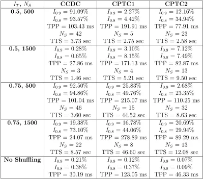
Table 4.1 shows the eﬀect of changing the shuﬄing trigger parameters on the

perfor-mance metrics using the three diﬀerent datasets.

The main trade-off in changing the shuffling trigger parameters is between shuffling

frequency and time. On average, the more frequently shuﬄing is allowed, the longer

the system takes to run. There is an example where this generalization is not true;

(42)

IT, NS CCDC CPTC1 CPTC2

0.5, 500 I0.9 = 91.09% I0.9 = 2.27% I0.9 = 12.16% I0.8 = 93.57% I0.8 = 4.42% I0.8 = 34.94%

TPP = 103.43 ms TPP = 191.91 ms TPP = 77.91 ms

NS = 42 NS = 5 NS = 23

TTS = 3.73 sec TTS = 2.75 sec TTS = 2.58 sec

0.5, 1500 I0.9 = 0.28% I0.9 = 3.10% I0.9 = 7.12%

I0.8 = 0.65% I0.8 = 8.15% I0.8 = 7.49%

NS = 3 NS = 4 NS = 13

0.75, 500 I0.9 = 92.50% I0.9 = 25.83% I0.9 = 2.68% I0.8 = 94.86% I0.8 = 49.76% I0.8 = 23.35%

NS = 46 NS = 15 NS = 32

0.75, 1500 I0.9 = 19.38% I0.9 = 16.78% I0.9 = 20.69% I0.8 = 73.10% I0.8 = 44.06% I0.8 = 29.94%

NS = 22 NS = 8 NS = 13

No Shuﬄing I0.9 = 0.21% I0.9 = 0.12% I0.9 = 0.07%

I0.8 = 0.38% I0.8 = 0.37% I0.8 = 0.09%

[image:42.612.124.525.71.422.2]

Table 4.1: Performance Metrics with Varying Shuﬄe Trigger Parameters

whereNI is 1,500 is higher than the case whereNI is 500. The reasoning for this can

be explained by examining the index graphs for these cases. The index graph for the

NI = 500 case can be seen in Figure 4.1 while the index graph for the NI = 1,500

case can be seen in Figure 4.2.

In these cases, it can be seen that, although shuﬄing occurs more frequently in the

NI = 500 case, the index is unable to rise above the 0.8 and 0.9 values. This is an

example on why the shuﬄing algorithm in its current iteration is not optimal.

Be-cause the shuﬄing algorithm does not have the ability to add models to the ASG, it is

possible that one model could represent multiple attack behaviors. It is also possible

that shuﬄing too frequently does not allow for a suﬃcient number of observables to

(43)

[image:43.612.147.503.76.288.2]

Figure 4.1: CPTC2 data with shuﬄe parametersIT = 0.75 and NI = 500

Figure 4.2: CPTC2 data with shuﬄe parametersIT = 0.75 and NI = 1500

In general, to select the parameters for shuﬄing it is preferred to allow enough time

between shuﬄing to allow for a suﬃcient number of packets to enter the system while

keeping the minimum index relatively high in order to allow for shuﬄing as the index

begins to fall.

The remainder of the results in Chapter 4 will be run with anIT of 0.75 and anNS of

[image:43.612.144.504.330.540.2]

(44)

the system using the MACCDC data and section 4.6 will be evaluating the eﬀect of

datasets on the system using both the MACCDC and CPTC datasets. These

param-eters were chosen because they provide clear examples to demonstrate the capabilities

of the system.

4.3 Eﬀect of Bayesian Prior

When classifying using Bayes’ Theorem, it is important to use an informative Bayesian

Prior in order to ensure accuracy of the classification. The Bayesian Prior by definition

is the probability of new evidence belonging to a model without bias based on the

features of the observable or the model. In this work, three Bayesian Priors were

explored. The first was a uniform prior based on the number of models. This is the

most naive prior for the system as it simply allows the likelihood calculation to fully

determine the classification of the edge to a model. The graph in Figure 4.3 shows the

uniform priors of each of the four models created by the system over each iteration

of packets entering the system.

[image:44.612.219.415.474.632.2]

The second Bayesian Prior explored was a prior based on the number of edges

Figure 4.3: Uniform Prior Over Iterations

in a model over the total number of edges in the ASG. This prior provides more

(45)

is more likely to have a new edge classified to that model. Figure 4.4 shows a graph

of the edge based priors for each of the four models over each iteration of packets

entering the system.

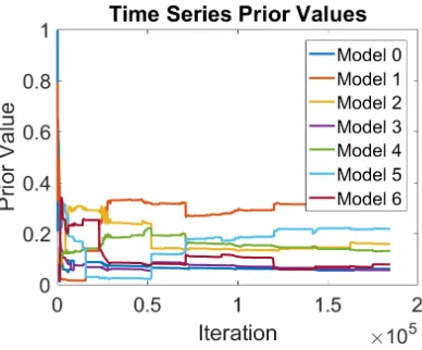
[image:45.612.218.414.175.333.2]

The third Bayesian Prior explored was the time series based prior defined in Section

Figure 4.4: Edge Based Prior Over Iterations

3.1.2. This Prior provides more information than the edge based prior as it takes into

account trends in the data. This prior assumes that models with more edges classified

recently will continue to grow while those that have not gained edges will continue

to maintain the edges that the models contain. Figure 4.5 shows a graph of the time

series based prior over iterations of the system.

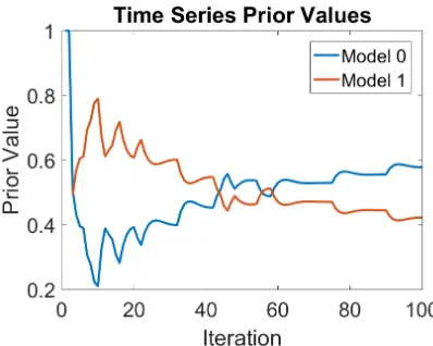
Upon examination of the graphs of the edge based and time series based priors, the

[image:45.612.220.414.531.692.2]

(46)

two priors appear to be identical. Looking closer at individual prior values it can be

seen that this is not the case. Figure 4.6 and Figure 4.7 show the prior values for two

models in the first 100 iterations of the system using the edge based prior and the

time series based prior respectively.

[image:46.612.218.417.406.565.2]

From these two graphs it can be seen that the prior values using the edge based and

Figure 4.6: 100 Iterations Edge Based Prior

Figure 4.7: 100 Iterations Time Series Based Prior

time series based priors are similar but are, in fact, diﬀerent. This is to be expected

as both prior values depend on the number of edges in the models to calculate the

prior. Comparing these two graphs also clearly shows the eﬀect of trends on the time

series based prior.

(47)

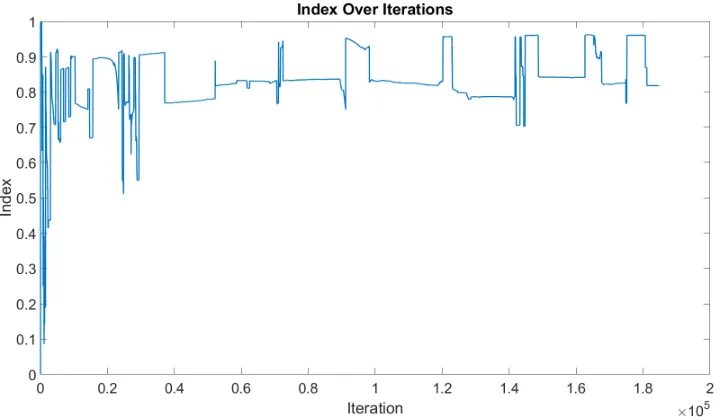
over each iteration of the system were created using each of the three diﬀerent priors.

Figure 4.8 shows the index graph using the uniform prior. Figure 4.9 shows the index

graph using the edge based prior. Figure 4.10 shows the index graph using the time

series based prior.

[image:47.612.146.504.204.412.2]

Examining these graphs, the index values for all three priors appear to be very

[image:47.612.144.504.469.679.2]

Figure 4.8: Index Using Uniform Prior

(48)

[image:48.612.145.505.75.292.2]

Figure 4.10: Index Using Time Series Based Prior

Index Value Uniform 0.19232445376286245

Edge 0.19232445376286256

Time Series 0.19232445376286247

Table 4.2: Index Value at Iteration 1,501 Using Diﬀerent Priors

similar. This is expected as the posterior is driven mainly by the likelihood calculation

in Bayes’ Theorem. Table 4.2 shows an example of the index values at iteration 1,501

to show the eﬀect of the diﬀerent Bayesian Priors.

The diﬀerent Bayesian Priors were also examined using the relevant performance

metrics explained in Section 4.1.2. Table 4.3 shows the comparison of the three

diﬀerent priors using these performance metrics.

Using these metrics, it can be seen that changing the prior has little eﬀect on the

overall performance of the system. Again, this is as expected because of the idea in

I0.9 I0.8 TPP Uniform 19.38% 73.10% 28.79 ms

Edge 19.38% 73.10% 27.85 ms

Time Series 19.38% 73.10% 27.16 ms

(49)

Bayes’ Theorem that the likelihood value should drive classification. The purpose of

the Bayesian prior is to determine which model is more likely to have new observables

classified to it in cases where the likelihood is very similar between models. For this

reason, the prior that provides more information about the models should be used

which, in this system, is the time series based prior.

4.4 Dynamic Model Generation

Because of the nature of the data having no ground truth data about the number

or composition of models, model creation is an important piece of the system. The

ability to dynamically generate models while data enters the system is essential for

the accuracy of the classification. A new model is to be generated when an observable

enters the system that does not fit well into any existing model. To demonstrate the

capability of the system to dynamically generate models, an example is shown where

three models exist and a new edge is created with features not prevalent in the existing

models. Figures 4.11 through 4.13 show the features present in the existing models.

The next edge to be created in the system is one with destination port 57,989,

Figure 4.11: Model 0 Features

source port 55,553, and TCP protocol, a feature combination not prevalent in any

of the existing models. The posteriors of the edge belonging to one of the existing

models are shown in Table 4.4.

(50)

[image:50.612.106.545.218.332.2]

where the edge is classified to the highest posterior model, Model 2 in this example,

or a new model is created from the edge. Table 4.5 shows the index comparison for

this example.

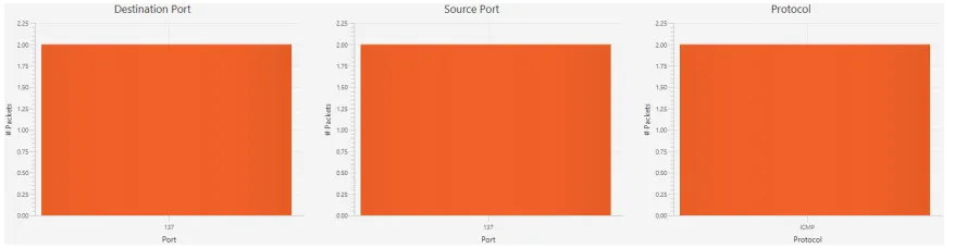
Because the index value when a new model is created is larger, the new model is

introduced to the system. Figure 4.14 shows the features for the newly created model

showing the success of the dynamic model generation process.

Although the feature graphs for Model 2 and the new model appear to be very similar,

it is the values in these feature graphs that separate the two. Model 2 contains edges

with source port 137, destination port 137, and ICMP Protocol. The new edge and,

therefore, new model contain source port 55553, destination port 57989, and TCP

Posterior Model 0 6.285×10−7

Model 1 1.138×10−7

Model 2 0.9999

(51)

Index Value Classification to Existing Model 0.333

Creation of New Model 0.4191

Table 4.5: Index Comparison for Model Generation

Figure 4.14: New Model Features

Protocol.

4.5 Model Shuﬄing

During the classification process, it is reasonable to assume that misclassification of

edges could occur. This is particularly true with no ground truth knowledge of the

models determining the features that should be present in each individual model.

Be-cause of this, it is important to have the ability to periodically reevaluate the models

the edges are classified to. Figure 4.15 shows an example of the index over iterations

in a system where shuﬄing is present. Figure 4.16 shows an example of the index

over iterations when shuﬄing does not occur. When comparing the two graphs, the

importance of shuﬄing is seen as the shuﬄing gives the ability for the index to rise

during the classification. This can also be seen in Table 4.1 comparing the cases where

shuﬄing is present to the case where no shuﬄing occurs.

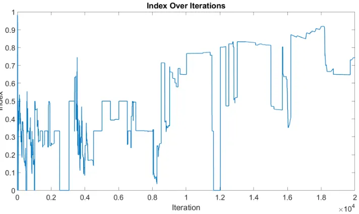
To demonstrate the ability of the system to shuﬄe edges into models an example

is shown where the index falls below the threshold and the shuﬄing occurs after the

proper number of iterations. Figure 4.17 shows the index value leading up to and

(52)

[image:52.612.153.503.76.288.2]

Figure 4.15: Index Over Iterations with Shuﬄing

Figure 4.16: Index Over Iterations with no Shuﬄing

though the index falls below the threshold of 0.75 before that. This occurs because

the parameter determining the minimum iterations between shuﬄing is set to 1,500.

From this graph, the shuﬄing can easily be seen to have occurred as the index

sharply rises. This happens because the posteriors of the edges belonging to the new

models they are classified to are much higher than the models that existed before

[image:52.612.144.502.326.539.2]

(53)

[image:53.612.147.507.76.286.2]

Figure 4.17: Index at Shuﬄing

After shuﬄing, the models that were present before shuﬄing and those that exist

after are quite diﬀerent. Figures 4.18 through 4.24 show the features of the existing

models before shuﬄing for the above example. Figures 4.25 through 4.28 show the

features of the models after shuﬄing occurs. Clearly, after shuﬄing, the models are

much diﬀerent than before. For example, all edges with a source port of 137,

con-tained in Models 2, 3, and 5 before shuﬄing, are in the same model, Model 5, after

shuﬄing. The same type of shift can be seen in the protocol feature as well as all

edges containing packets with an ICMP protocol, originally contained on Models 1,

2, 3, and 5, are contained in Model 5 after shuﬄing.

[image:53.612.112.541.573.685.2]

(54)

[image:54.612.112.540.70.183.2]

[image:54.612.107.540.236.350.2]

Figure 4.19: Model 1 Features Before Shuﬄing

[image:54.612.103.546.400.512.2] [image:54.612.109.542.563.677.2]

(55)

[image:55.612.108.542.70.184.2] [image:55.612.108.542.235.347.2]

Figure 4.25: Model 0 Features After Shuﬄing

[image:55.612.111.541.398.510.2] [image:55.612.110.542.559.673.2]

(56)

[image:56.612.107.544.72.184.2]

[image:56.612.108.543.237.345.2]

[image:56.612.112.541.397.508.2] [image:56.612.110.543.559.672.2]

Dynamic Model Generation and Classification of Network Attacks

Dynamic Model Generation and Classification of

Network Attacks

Jacob D. Saxton

Dynamic Model Generation and Classification of

Network Attacks

Dynamic Model Generation and Classification of

Network Attacks

Contents

List of Figures

List of Tables

Introduction

Chapter 2

Related Works

2.1

Network Attack Recognition

2.2

Attack Social Graph and the NASS Framework

2.3

Clustering

2.4

Classification of Streaming Data

Methodology

3.1

Dynamic Bayesian Classifier

3.2

Dynamic Model Generation

3.3

Model Shuﬄing

3.4

System Flow

Results

4.1

Design of Experiments

4.2

Eﬀect of Changing Shuﬄing Trigger Parameters

4.3

Eﬀect of Bayesian Prior

4.4

Dynamic Model Generation

4.5

Model Shuﬄing