DYNAMIC MODEL ON THE SPREAD OF BOTS FOR AN E COMMERCE NETWORK

(1)

Volume 8, No. 7, July – August 2017

International Journal of Advanced Research in Computer Science

RESEARCH PAPER

Available Online at www.ijarcs.info

ISSN No. 0976-5697

DYNAMIC MODEL ON THE SPREAD OF BOTS FOR AN

E-COMMERCE NETWORK

Biswarup Samanta

Samir Kumar Pandey

Department of Computer Science & Engineering Department of Mathematics Amity University Jharkhand, Rnachi, India XIPT, Ranchi, Jharkhand, India

Abstract— The primary goal of e-commerce network is to sell goods and services online.Increasing usages of e-commerce network increases the security loop holes in the network. Nodes of an e-commerce network can be easily compromised by various types of malware. The nature of the spread of malware among the nodes of an e-commerce network can be easily compared with the spread of biological viruses (infectious diseases) within human population of any locality. So we can easily apply the epidemic model for the spread of infectious disease within human population into the spread of malware among the nodes of a computer network. Various types of malware are used to attack the network of an organization, but, here, in this paper we concentrate and formulate a dynamic model for the propagation of bots in an e-commerce network and study its dynamic behavior. After categorizing the nodes of the network, based on their interface to the Internet, we have proposed two sub-models to formulate the overall architecture of the model. A schematic compartmental model is designed to represent the propagation of bots within the network and then differential equation model is formulated to represent the dynamics of all the compartments, respectively. The proposed system is solved and the basic reproduction number is also calculated to analyze the stability of the system. At the end, we have shown the result of numerical simulations using MATLAB to support the dynamism of our proposed model.

Keywords— cyber-attack, malware, bots, dynamic model, e-commerce, stability I.INTRODUCTION

E-commerce has presented a new way of doing business all over the world using Internet. It refers to a wide range of online business activities for products and services. It is a powerful tool for business transformation that allows companies to enhance their supply-chain operation, reach new markets, and improve services for customer as well as for providers [10]. Commercial activities over the Internet have been growing in an exponential manner over the last few years. As the world becomes more electronically connected, systems running on network become more vulnerable to cyber-attack and this has posted a serious challenge for information security. Web based attacks are considered to be the greatest threat to any business or state as it is related to the confidentiality, availability, and integrity of the data for the business and the state, respectively.

Major types of cyber-attacks on e-commerce network includes fraudulent-email, pharming, snooping the shopper’s computer, malware, man in the middle attack, Cross Site Scripting (CSS), password attacks, etc. Here, in this paper, we concentrate on a specific type of malware attack, known as bots attack, which is the basis for formulation of our proposed model and its solution, is discussed throughout the remaining portion of this paper.

There are many different classes of malware that have varying ways of infecting systems and propagating themselves. Some of the more commonly known types of malware are viruses, worms, Trojans, bots, back doors, spyware, and adware. A malicious bot is self-propagating malware designed to infect a host and connect back to a central server or servers that act as a command and control (C&C) center for an entire network of compromised devices, known as "botnet”. The term botnet comes from

robot net

In this section we will develop a model on the attack and spread of bots among the nodes within an e-commerce network. Several mathematical models have been developed which give clear view of attacking behavior as well as the transmission of malicious codes in network [1-9]. A typical e-commerce network consists of various types of computers, viz.; workstations, servers, routers and other devices also. Server may be of different types, viz.; web server, database server, application server, mail server, etc. All the servers are internal to the network, i.e.; they are not directly connected to the outside world. Apart from the servers there are some other workstations which are internal to the network and forms the backbone of the network, i.e.; an attacker or a valid client can’t directly interact with those nodes also. But there will be some other computers (external nodes) which are the interfaces to the backbone of that network, i.e.; an attacker or a valid client can directly connect to those computers with the help of the Internet. A

work. The computers under the botnet are the collection of computers that are connected to the internet and have been compromised by a cracker, computer virus, bots or Trojan horse and can be used to perform malicious tasks of one sort or another under the control of a remote server known as “bot herder” or “bot master” or “command-and-control (C&C) server”. In most of the cases the owner of the systems of botnet are unaware that their systems are being used in this way and hence, these computers are metaphorically compared to zombies. The zombie computers of the botnet, which are controlled by a C&C server, are used to forward transmissions, including spam, viruses or worms to other computers on the e-commerce network. Bots have all the advantages of worms, but are generally much more versatile in their infection vector, and are often modified within hours of publication of a new exploit [14].

(2)

bot master or C&C server first target those interface nodes of that network and turn them to zombie computers with the help of bots and turn them to the part of its botnet. Now those zombies will be controlled by the bot master. The bot master, with the help of those zombies, can infect other computers of that network by transmitting bots throughout the network and can reach and infect the targeted server of that network to make the entire network to crash. This scenario can be represented schematically as shown in the following fig. 1.

Considering the above discussed scenario, we have created a schematic model consisting of two different, but interactive models. Before we proceed with the mathematical modeling of the above mentioned framework, we briefly discuss the basic assumption which will guide our formulation of equation system as follows.

Dynamic model for infectious diseases are mostly based on compartment structures that were initially proposed by Kermack and McKendrick [11-13] and later developed by other mathematicians. To formulate a dynamic model on the transmission of an epidemic disease, the entire population in a given region is often divided into several different groups or compartments. In this paper we apply “S-I-S” model for the population of the external computers which are directly connected to the Internet. Initially all the external nodes which are directly connected to the outside of the network through Internet are placed in “S” class. But, once a node of “S” class is infected by the bots sent from a “C&C server” to turn it into a zombie computer, that node is transferred into the “I” class. As the non-availability of the external node directly affect the services it provides to its client nodes, the nodes in the “I” class of our “S-I-S” model are repaired immediately with the help of antimalware software or any other means of repair and hence it is transferred back to the “S” class to resume its operation.

The population of the internal nodes of our e-commerce network is used to form the “S-I-Q-S” model. Initially all the internal nodes of our network are placed into the “S” class. The nodes of that “S” class may be affected by the zombies of the “S-I-S” model. Once, a node from “S” class is infected by the zombies of “S-I-S” model, it is transferred into the “I” class. The nodes of the “I” class are quarantined and transferred into “Q” class. The non-availability of the internal nodes may hamper the communication process within the network and hence the quarantine nodes are repaired immediately and transferred to the “S” class again to resume their operation. The entire population of the computers of our network is divided into the following five compartments:

(i) Susceptible-External (Se): represents the external nodes

which are susceptible to direct attack from bots of an existing botnet.

(ii) Infectious-External (Ie): represents the infected external

nodes which are infectious and are capable of spreading the bots to other susceptible nodes.

(iii) Susceptible-Internal(S): represents the internal nodes which are susceptible to the attack from the zombie computers of the botnet.

(iv) Infectious-Internal (I): represents the infected internal nodes which are infectious and are capable of spreading the bots to other susceptible nodes.

(v) Quarantine (Q):represents the internal nodes which are infected and separated.

The study of epidemic dynamics is an important theoretic approach to investigate the transmission dynamics of infectious diseases. It formulates mathematical models to describe the mechanism of disease transmissions and dynamics of infectious agents. Different transmission rates which are used to show the dynamism of our model are as follows: b: birth rate as well as death rate of the suspected external nodes; β: transmission rate coefficient; α: quarantine rate coefficient; σ: loss of immunity rate coefficient; µ: death rate of external nodes due to attack. The corresponding model equations for Internal Nodes of an E-Commerce Network (S–I–Q-S) are given in the following system equation:

.

,

Q

I

dt

dQ

I

SI

dt

dI

Q

SI

dt

dS

e e

σ

α

β

σ

β

−

=

−

=

+

−

=

(1)

For the above system (1), we may assume the following equation,

1 .

1

I S Q

Q I S

− − = ⇒

= + +

(a)

In the above equation (a), S, I and Q represents the fraction of the total nodes from susceptible, infectious and quarantine categories, respectively, present in the internal part of an e-commerce network of an organization.

The corresponding model equations for External Nodes of an E-Commerce Network are given in the following system equations:

. ) (

,

e e

e e e

e e e e e

I b I I S dt dI

I I S bS b dt dS

µ

α

β

σ

β

+ − − =

+ −

− =

(2)

For the above system (2), we may assume the following equation,

1 .

1

e e

I S

− = ⇒

= +

(b)

In the above equation (b), Se, and Ie represents the

(3)

categories, respectively, present in the external part of an e-commerce network of an organization. By using the equations (a) and (b), respectively, we may simplify the above mentioned two systems equations, viz.; (1) and (2), into the following system equation:

.

)

(

)

1

(

,

),

1

(

e e e e e e e

I

b

I

dt

dI

I

SI

dt

dI

I

S

SI

dt

dS

µ

α

β

α

β

σ

β

+

−

=

−

=

−

+

−

=

(3)

Let U be used to represent the feasible region for the corresponding system (3) for the model given in the fig.1. Hence we may write U as follows:

).

1

,

1

,

0

,

0

,

0

:

)

,

((

∈

3

>

≥

+

≤

=

S

I

_e

R

S

I

_e

S

I

_e

U

III.SOLUTIONANDBASICREPRODUCTION

NUMBER

In this section, we discuss about the solution of the system developed and find out the basic reproduction number, which helps us to analyze the stability of the system.

A. Solution of the System (Calculation of Equilibrium Points)

To calculate the equilibrium points for the proposed model, we set the right sides of the model equations of system (3) equal to zero, that is,

0

=

dt

dS

,

0

=

dt

dI

,

.

0

=

dt

dI

_e

Using the above mentioned three equations, the trivial bots free equilibrium is obtained at point E1 ≡ (1, 0, 0) and the

endemic equilibrium is found at point E2 ≡ ( S*, I*, Ie*),

where,

,

)

)(

(

*

σα

µ

α

β

σ

α

ασ

+

−

+

=

b

S

, ) )( ( ) ( *

σα

µ

α

β

σ

α

µ

α

β

σ

+ − − − − − − − = b b I

.

*

β

µ

α

β

−

=

b

I

_e

B. Basic Reproduction Number

The basic reproduction number, also known as threshold number, is defined by the average number of secondary infections produced by one infected node of a network during the mean course of infection in completely susceptible nodes of the network. This is also simply known as reproductive number and is denoted by R0. The essential

condition for an epidemic to occur is that the number of

infected nodes should increase i.e. _>₀_.

dt dI

We get the following equation for the changes of infected nodes over time from system (1) as follows:

. I SI dt dI e α β −

= (1.1)

By applying the above condition for an epidemic to occur on the above mentioned equation (1.1) we get

. 1 0 0 > ⇒ > − ⇒ > I SI I SI dt dI e e

α

β

α

The above condition is satisfied when ₁ 0 =_α >

β

R , because

the transmissions to infectious nodes are greater than the transmission to quarantine node. Similarly from the system (2) we have the following equation

.

)

(

_e e e e

e

S

I

b

I

dt

dI

β

α

µ

+

−

=

(2.1)

By applying the condition for an epidemic to occur on the above mentioned equation (2.1) we get,

0

)

(

0

>

+

−

⇒

>

e e e e e

I

b

I

S

dt

dI

µ

α

β

IV.STABILITYOFTHESYSTEM

In this section we discuss the local stability at bots free equilibrium as well as at endemic equilibrium.

Theorem 1. The malware free equilibrium E1 of system (3)

is locally asymptotically stable in U if R₀_e <1 and is unstable if R0e >1.

Proof. Linearizing system (3) around the malware free equilibrium point E1 ≡ (1, 0, 0), we obtain the following

Jacobian matrix













+

−

=

)

(

0

1

µ

α

β

α

β

σ

b

J

E

To examine the local stability of the equilibria of system (3), for its Jacobian matrix JE1, we need to find out its

eigenvalue. The characteristic equation for the above matrix (JE1) is given as follows:

.

0

))

)(

)((

)

(

β

−

α

+

b

+

µ

−

λ

−

σ

−

λ

−

α

−

λ

=

Hence the characteristic roots are .

, ),

( 2 3

1 β α µ λ σ λ α

λ = − +b+ =− =− As we know

.

0

α

µ

(4)

that, σ and α are always positive, so the second (λ2) and third

(λ3) Eigen values are negative.

Let us assume that the first Eigen value (λ1) is also negative,

i.e. β −(α +b+µ)<0, which is equivalent to ₁ 0e < R and that can be proved as follows:

.

1

)

(

0

)

(

0

<

⇒

<

+

⇒

+

<

⇒

<

+

−

e

R

b

µ

α

β

µ

α

β

µ

α

β

Hence our assumption is true, that is the first Eigen value is also negative. Thus all the Eigen values of the Jacobian Matrix JE1 at the equilibrium E₁≡(1,0,0) are negative, and

hence the malware free equilibrium is locally asymptotically stable, if R0e <1. On the other hand, ifβ >(α +b+µ), then the first Eigen value (λ1) is

positive, i.e.

Hence the equilibrium point E1 ≡ (1, 0, 0) becomes

unstable, if ₁ 0e >

R .

Theorem 2.The endemic equilibrium E2 of system (3) is

locally asymptotically stable in U, ifR0e >1.

Proof. Following the same way as above Theorem 1, the system (3) is linearized at the endemic equilibrium point

) , , ( * * *

2 S I Ie

E ≡ to obtain the following Jacobian matrix













+

−

+

−

=

)

(

2

0

*

* *

2

µ

α

β

α

β

σ

β

b

I

S

I

S

I

J

e e

e

E

The characteristic equation for the above matrix (JE2) is

given as follows:

0 } ) )( }{(

) (

2

{− βI_e*+β− α+b+µ −λ βI_e*+σ+λ α+λ +σβI_e* =

One of the Eigen values of the Jacobian Matrix JE2 at the

equilibrium ₍ *_, *_, *₎

2 S I Ie

E ≡ is found as follows:

).

(

2

*

1

β

α

µ

λ

=

−

I

_e

+

−

+

b

+

Let us assume that

λ

1

<

0

, i.e.

.

0

)

(

2

*

+

−

+

<

−

β

I

_e

β

α

b

µ

After putting the value of Ie* in the above equation, we

get,

β

µ

α

µ

α

β

µ

α

β

µ

α

β

µ

α

β

µ

α

β

<

+

⇒

<

+

−

⇒

<

+

−

+

−

⇒

<

+

−

+

−

)

(

0

)

(

0

)

(

)

(

2

0

)

(

2

b

⇒

α

+

β

b

+

µ

<

1

. 1

> + + ⇒

µ

α

β

b

That is,

R

0e

>

1

.

Hence the above assumption is true, i.e.; the first Eigen value

λ

1

=

−

2

β

I

e*

+

β

−

(

α

+

b

+

µ

)

is negative. The

other two Eigen values (λ2, λ3) will be the roots of

0 ) ) )( )((

) (

2

(₋ *₊ ₋ ₊ ₊ ₋ *₊ ₊ ₊ ₊ * ₌

e e

e b I I

I β α µ λ β σ λ α λ σβ

β

, which is the characteristic equation of JE2. Since the sum of

those two roots (λ2, λ3) is negative and the product of the

roots is positive, therefore suggesting that both of its roots λ2

and λ3 are negative. So, all the three Eigen values of JE2 are

negative when ₁ 0e >

R . Hence the endemic equilibrium E2

is locally asymptotically stable, if ₁ 0e>

R _.

V.SIMULATIONANDDISCUSSION

In this section we will show the result of numerical simulations using MATLAB to support the dynamism of our formulated model.

A. Stability at Bots Free Equilibrium

The dynamic behavior of the entire population of system (3) is examined through simulation and the result is displayed in fig.2. The simulation is done for three different initial conditions, (S, I, Ie) ≡ ((0.3,0.5,0.2), (0.5,0.3,0.2),

(0.7,0.2,0.1)) and we get the resultant data about the number of computer in different classes for all of the above three conditions as follows, (S, I, Ie) ≡ ((1.000,0.000,0.000),

(1.000,0.000,0.000), (1.000,0.000,0.000)), i.e., final states are

same for all the conditions and there are no infectious nodes present in the system when R0e < 1. At this point the system

is stable because all the bots are wiped out from the system and hence our proposed model is found to be asymptotically stable at R0e < 1.

.

1

)

(

0

>

⇒

>

+

⇒

+

>

e

R

b

µ

α

β

µ

α

(5)

[image:5.595.37.260.72.242.2]

Fig. 2 Local stability for bots free equilibrium of system equation (3), when 1

0e <

R (when, β=0.012;α=0.010; b=0.020; μ=0.010).

B. Stability at Endemic Equilibrium

The stability of endemic equilibrium point is shown in fig. 3 for three different initial conditions same as fig. 2. Here also, we get the unique final states for all the given conditions as follows: (S, I, Ie) ≡ ((0.0100, 0.2475, 0.9250),

(0.0100, 0.2475, 0.9250), (0.0100, 0.2475, 0.9250)). Hence the system is stable at this point, though the bots exists in the system. It is also found from the fig.3 that the system is asymptotically stable at this point when R0e > 1.

0 100 200 300 400 500 600 700 800 900 1000 0

0.1 0.2 0.3 0.4 0.5 0.6 0.7 0.8 0.9 1

Time --->

C

la

ss

es

o

f N

od

es

--->

S1 I1 Ie1 S2 I2 Ie2 S3 I3 Ie3 I1,I2,I3

Ie1,Ie2,Ie3

[image:5.595.334.532.89.265.2]

S1,S2,S3

Fig. 3 Local stability for endemic equilibrium of system equation (3), when 1

0e >

R (when, β=0.800; α=0.030; b=0.020; μ=0.010)

C. Bots Free Equilibrium for System (1) & (2)

To observe the effect of increase in β on the dynamisms of the classes of nodes in system (1) & (2), we simulate the models using two different values of β (0.12, 0.92) for a given initial point (S, I, Q, Se, Ie) ≡ (0.4, 0.2, 0.1, 0.2, 0.1)

and the given value of (σ, α, b, μ) ≡ (0.01, 0.03, 0.02, 0.01) and we get two different set of values of (S, I, Q, Se, Ie) ≡

((0.1667, 0.1333, 0.4000, 0.5000, 0.2000) and (0.0149, 0.0173, 0.5138, 0.0652, 0.03739)).

From our resultant data we can say that our proposed system become stable at R0 > 1 due to the increase of

quarantine nodes from Q1 to Q2, where Q2 > Q1, as β is

increased from 0.12 to 0.92. It is also observed from fig.4,

that the system is asymptotically stable at R0 > 1, but bots

till exists in the system.

0 100 200 300 400 500 600 700 800 900 1000 0

0.1 0.2 0.3 0.4 0.5 0.6 0.7

Time --->

C

las

ses

of

N

odes

in S

ys

tem

(

1)

&

(

2)

-

-->

S1 I1 Q1 Se1 Ie1 S2 I2 Q2 Se2 Ie2

Q1 Q2

Fig. 4 Effect of increasing β on system dynamics at R0 > 1.

D. Dynamics of Infectious-Internal (I) nodes while changing the value of β

Fig.5. shows the result of simulation for the evolution of I over time at initial point (S, I, Ie) ≡ (0.7, 0.2, 0.1). We get

the following five sets of values of (S, I, Ie) ≡ ((0.0968,

0.2258, 0.5385), (0.0857, 0.2268, 0.5714), (0.0769, 0.2308, 0.6000), (0.0698, 0.2326, 0.6250), (0.0638, 0.2340, 0.6471)), for five different values of β = (0.13, 0.14, 0.15, 0.16, 0.17) and fixed value of σ = 0.01, α = b, μ = 0.01. It is found from fig. 5. , that the number of bots increases as β increases over time but the system becomes stable after a certain point of time and it proves that the endemic equilibrium is asymptotically stable at R0e > 1.

0 50 100 150 200 250 300 350 400 450 500

0.2 0.25 0.3 0.35 0.4 0.45 0.5

Time ---->

In

fe

c

ti

o

u

s

-I

n

te

rn

a

l (I

) ---->

beta=0.13 beta=0.14 beta=0.15 beta=0.16 beta=0.17 beta=0.17

[image:5.595.62.253.430.577.2]

beta=0.13

Fig. 5 Evolution of I over time, while β increases at R0e> 1; (β =

0.13/0.14/0.15/0.16/0.17, σ = 0.01, α = b, μ = 0.01).

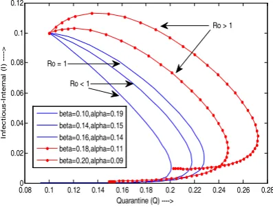
E. I VS Q by changing the values of β and α

The dynamisms of I vs. Q while changing the values of β and α to satisfy the following two conditions, i.e. R0e ≤ 1

and R0e > 1, are shown in fig. 6 and the resultant data of the

simulation are presented in Table 1.

0 100 200 300 400 500 600 700 800 900 1000

-0.2 0 0.2 0.4 0.6 0.8 1

Time --->

S1 I1 Ie1 S2 I2 Ie2 S3 I3 Ie3 S3

S2 S1

Cl

as

se

s o

f N

od

es

[image:5.595.324.519.493.650.2]

(6)

0.080 0.1 0.12 0.14 0.16 0.18 0.2 0.22 0.24 0.26 0.28 0.02

0.04 0.06 0.08 0.1 0.12

Quarantine (Q) ---->

In

fe

c

ti

o

u

s

-I

n

te

rn

a

l (I

) ---->

beta=0.10,alpha=0.19 beta=0.14,alpha=0.15 beta=0.16,alpha=0.14 beta=0.18,alpha=0.11 beta=0.20,alpha=0.09

Ro > 1

Ro = 1

[image:6.595.55.254.64.215.2]

Ro < 1

Fig. 6 Dynamics of I Vs Q when R0e > 1 and R0e≤ 1

It is found from the following Table 1, that there will be no bots in the system when R0e ≤ 1, which is a bots free

equilibrium state and bots exists when R0e > 1, i.e.; endemic

equilibrium state. Fig. 6 also shows that the bots free equilibrium is asymptotically stable when R0e ≤ 1 and

endemic equilibrium is also asymptotically stable when R0e

> 1.

TABLE 1. RESULT OF “I” vs. “Q” SIMULATION

σ μ b α β R0e S I Q Se Ie

0.01 0.01 0.01 0.19 0.1 < 1 0.5073 0 0.0927 0.6999 0 0.01 0.01 0.01 0.15 0.14 < 1 0.4909 0 0.1091 0.6912 0 0.01 0.01 0.01 0.14 0.16 = 1 0.4813 0 0.1187 0.6853 0 0.01 0.01 0.01 0.11 0.18 > 1 0.4497 0.0012 0.1491 0.6619 0.0014 0.01 0.01 0.01 0.09 0.2 > 1 0.3879 0.0099 0.2022 0.6023 0.0123

VI.CONCLUSION

In this paper, we have formulated an epidemic model to study the dynamics of the spread of bots in an e-commerce network through botnet. Categorizing the nodes of the networks based on their interface to the Internet, we have formulated two sub systems to represent the entire system for the propagation of bots. We have observed that if the basic reproduction number is less than unity, then the system is bots free and the bot free equilibrium is locally asymptotically stable. It is also found that when the reproduction number is greater than one, the system is also stable although bots persist in the system. During the analysis of the dynamism of the proposed model it is also found that the Infectious-Internal nodes are increased up to a certain peak over a period of time, but after a certain point of time it stabilizes. And while analyzing the dynamism of

Infectious nodes over the Quarantine nodes by increasing the infectivity contact rate, it is found that bots can exists in the system if R0e > 1, but the system is bots free when R0e≤

1.

VII. REFERENCES

[1] B.K. Mishra, S.K. Pandey, Dynamic Model of worms with

vertical transmission in computer network, Appl. Math. Comput. 217 (21) (2011) 8438–8446, Elsevier.

[2] B.K. Mishra, S.K. Pandey, Fuzzy epidemic model for the

transmission of worms in computer network, Nonlinear Anal.: Real world Appl. 11 (2010) 4335–4341.

[3] B.K. Mishra, S.K. Pandey, Effect of antivirus software on

infectious nodes in computer network: a mathematical model, Phys. Lett. A 376 (2012) 2389–2393. Elsevier.

[4] B. Samanta, S. K. Pandey; Attacking Behaviour of Computer

Worms on E-Commerce Network : A Dynamic Model; IJRASET; Vol. 2 Issue XII, Dec 2014.

[5] Erol Gelenbe, Varol Kaptan, YuWang, Biological metaphors

for agent behaviour, in: Computer and Information SciencesISCIS 2004, 19th International Symposium, in: Lecturer Notes in Computer Science, vol. 3280, Springer-Verlag, 2004, pp. 667-675.

[6] J.R.C. Piqueira, B.F. Navarro, L.H.A. Monteiro,

Epidemiological models applied to virus in computer network, J. Comput. Sci. 1 (1), 2005, 31-34.

[7] Y.Wang, C.X.Wang, Modelling the effect of timing

parameters on virus propagation, in: 2003 ACM Workshop on Rapid Malcode, ACM, 2003, pp. 61-66.

[8] S. Forest, S. Hofmeyr, A. Somayaji, T. Longstaff,

Self-nonself discrimination in a computer, in: Proceeding of IEEE Symposium on Computer Security and Privacy, 1994, pp. 202-212.

[9] Bimal K. Mishra, Navnit Jha, SEIQRS model for the

transmission of malicious objects in computer network, Appl. Math. Model. 34 (2010) 710-715.

[10]S. Yasin, K. Haseeb, R. Qureshi; “Cryptography Based

E-Commerce Security: A Review”; IJCSI; V0l. 9, Issue 2, No 1, March 2012.

[11]W.O. Kermack, A.G. McKendrick, Contributions of

mathematical theory to epidemics, Proc. R. Soc. Lond. Ser. A 115, 1927, 700-721.

[14]

[image:6.595.34.298.369.459.2]