White Rose Research Online URL for this paper:
http://eprints.whiterose.ac.uk/97993/
Version: Accepted Version
Article:
Rahm, A.D. and Sengun, M.H. (2013) On Level One Cuspidal Bianchi Modular Forms.
LMS Journal of Computation and Mathematics, 16. pp. 187-199. ISSN 1461-1570
https://doi.org/10.1112/S1461157013000053
[email protected] https://eprints.whiterose.ac.uk/ Reuse
Unless indicated otherwise, fulltext items are protected by copyright with all rights reserved. The copyright exception in section 29 of the Copyright, Designs and Patents Act 1988 allows the making of a single copy solely for the purpose of non-commercial research or private study within the limits of fair dealing. The publisher or other rights-holder may allow further reproduction and re-use of this version - refer to the White Rose Research Online record for this item. Where records identify the publisher as the copyright holder, users can verify any specific terms of use on the publisher’s website.
Takedown
If you consider content in White Rose Research Online to be in breach of UK law, please notify us by
arXiv:1104.5303v3 [math.NT] 19 Feb 2013
ALEXANDER D. RAHM AND MEHMET HALUK ŞENGÜN
Abstract. In this paper, we present the outcome of vast computer cal-culations, locating several of the very rare instances of level one cuspidal Bianchi modular forms that are not lifts of elliptic modular forms.
Bianchi modular forms over an imaginary quadratic field K are auto-morphic forms of cohomological type associated to the Q-algebraic group ResK/Q(SL2). Even though modern studies of Bianchi modular forms go
back to the mid 1960’s, most of the fundamental problems surrounding their theory are still wide open. In this paper, we report on our remarkably ex-tensive computations that show the paucity of genuine level one cuspidal Bianchi modular forms.
Let Sk(1) denote the space of level one weight k+ 2 cuspidal Bianchi
modular forms over K = Q(√−d). In their recent paper [FGT10], Finis, Grunewald and Tirao computed the dimension of the subspace Lk(1) of Sk(1) which is formed by (twists of) those forms which arise from elliptic
cuspidal modular forms via base-change or arise from a quadratic extension of K via automorphic induction (see [FGT10] for these notions). In this paper, we investigate numerically how much ofSk(1)is exhausted byLk(1).
There have been previous reports, however of limited size, in the 2009 paper [CM09] of Calegari and Mazur (the computations in this paper were carried out by Pollack and Stein) and in the 2010 paper [FGT10] of Finis, Grunewald and Tirao. While the computations in [CM09] were limited to the cased= 2, the computations in [FGT10] covered ten imaginary quadratic fields. The precise scope of the computations in [FGT10] is given in Table 1 below.
d 1 2 3 7 11 19 5 6 10 14
k6 104 141 116 132 153 60 60 60 60 60
Table 1. Finis-Grunewald-Tirao test range
It was observed in [CM09] that for 2k 6 96, one has L2k(1) = S2k(1).
The computations of [FGT10] extended those of [CM09]. An interesting outcome of the data they collected is that except in two of the 946 spaces they computed, one hasLk(1) =Sk(1). The exceptional cases are(d, k) = (7,12)
Date: 20th February 2013.
The first author is funded by the Irish Research Council.
The second author is funded by a Marie Curie Intra-European Fellowship.
and (d, k) = (11,10). In both cases, there is a two-dimensional complement to Lk(1)insideSk(1).
Using a different and more efficient approach, we computed, over more than 800 processor-days, the dimension of 4986 different spaces Sk(1) over
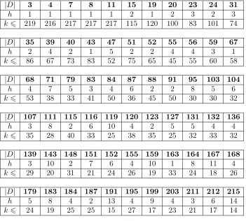
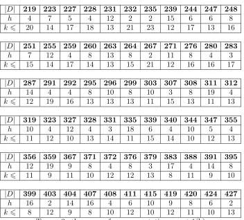
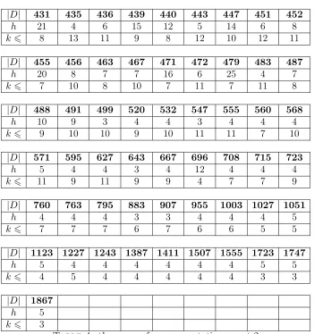
186 different imaginary quadratic fields. The precise scope of our computa-tions is given in Tables 2, 3 and 4, where D and h denote the discriminant and the class number of K respectively. In only 29 of these spaces were we able to observe genuine forms. The precise data about these exceptional cases is provided in Table 5.
|D| 3 4 7 8 11 15 19 20 23 24 31
h 1 1 1 1 1 2 1 2 3 2 3
k6 219 216 217 217 217 115 120 100 83 101 74
|D| 35 39 40 43 47 51 52 55 56 59 67
h 2 4 2 1 5 2 2 4 4 3 1
k6 86 67 73 83 52 75 65 45 55 60 58
|D| 68 71 79 83 84 87 88 91 95 103 104
h 4 7 5 3 4 6 2 2 8 5 6
k6 53 38 33 41 50 36 45 50 30 30 32
|D| 107 111 115 116 119 120 123 127 131 132 136
h 3 8 2 6 10 4 2 5 5 4 4
k6 35 28 40 33 25 38 35 25 32 33 32
|D| 139 143 148 151 152 155 159 163 164 167 168
h 3 10 2 7 6 4 10 1 8 11 4
k6 29 20 31 21 24 26 19 33 24 18 26
|D| 179 183 184 187 191 195 199 203 211 212 215
h 5 8 4 2 13 4 9 4 3 6 14
[image:3.612.132.483.241.557.2]k6 24 19 25 25 15 27 17 23 21 17 14
Table 2. the scope of our computations, part 1(a)
|D| 219 223 227 228 231 232 235 239 244 247 248
h 4 7 5 4 12 2 2 15 6 6 8
k6 20 14 17 18 13 21 23 12 17 13 16
|D| 251 255 259 260 263 264 267 271 276 280 283
h 7 12 4 8 13 8 2 11 8 4 3
k6 15 14 17 14 13 15 21 12 16 16 17
|D| 287 291 292 295 296 299 303 307 308 311 312
h 14 4 4 8 10 8 10 3 8 19 4
k6 12 19 16 13 13 13 11 15 13 11 13
|D| 319 323 327 328 331 335 339 340 344 347 355
h 10 4 12 4 3 18 6 4 10 5 4
k6 11 12 10 13 14 11 15 14 10 12 13
|D| 356 359 367 371 372 376 379 383 388 391 395
h 12 19 9 8 4 8 3 17 4 14 8
k6 11 9 11 10 12 12 13 8 11 9 10
|D| 399 403 404 407 408 411 415 419 420 424 427
h 16 2 14 16 4 6 10 9 8 6 2
[image:4.612.132.484.109.427.2]k6 8 12 9 8 10 12 10 12 11 10 13
Table 3. the scope of our computations, part 1(b)
non-trivial coefficients. Then to compute this cohomology space, we use the program Bianchi.gp [Rah10], which analyzes the structure of the Bianchi group via its action on hyperbolic 3-space (which is isomorphic to the as-sociated symmetric space SL2(C)/SU2). We then feed this group-geometric information into an equivariant spectral sequence that gives us an explicit description of the second cohomology of the Bianchi group, with the relevant coefficients.
|D| 431 435 436 439 440 443 447 451 452
h 21 4 6 15 12 5 14 6 8
k6 8 13 11 9 8 12 10 12 11
|D| 455 456 463 467 471 472 479 483 487
h 20 8 7 7 16 6 25 4 7
k6 7 10 8 10 7 11 7 11 8
|D| 488 491 499 520 532 547 555 560 568
h 10 9 3 4 4 3 4 4 4
k6 9 10 10 9 10 11 11 7 10
|D| 571 595 627 643 667 696 708 715 723
h 5 4 4 3 4 12 4 4 4
k6 11 9 11 9 9 4 7 7 9
|D| 760 763 795 883 907 955 1003 1027 1051
h 4 4 4 3 3 4 4 4 5
k6 7 7 7 6 7 6 6 5 5
|D| 1123 1227 1243 1387 1411 1507 1555 1723 1747
h 5 4 4 4 4 4 4 5 5
k6 4 5 4 4 4 4 4 3 3
|D| 1867
h 5
[image:5.612.132.483.106.480.2]k6 3
Table 4. the scope of our computations, part 2
generated. The second author thanks the Algebra and Geometry Group of the Mathematics Department of the University of Barcelona for the post-doctoral fellowship under which he carried out most of his work that went into this paper. Moreover, he thanks the Mathematical Sciences Research Institute of the University of California and the Max Planck Institute for Mathematics for the wonderful hospitality that he received during his stays. Finally, we would like to thank Frank Calegari, Lassina Dembélé for their comments on the paper and to Aurel Page for computing the Hecke action on the weight (1,1) cohomology for the fieldQ(√−199).
1. Background
|D| 7 11 71 87 91 155 199 223 231 339
k 12 10 1 2 6 4 1 0 4 1
dim 2 2 2 2 2 2 4 2 2 2
|D| 344 407 408 408 408 415 435 435 435 435
k 1 0 2 5 8 0 2 5 8 11
dim 2 2 2 2 2 2 2 2 2 2
|D| 455 483 571 571 643 760 1003 1003 1051
k 0 1 0 1 0 2 0 1 0
dim 2 2 2 2 2 2 2 2 2
Table 5. the cases where there are genuine classes
quotient hyperbolic 3-fold. The Borel-Serre compactification, see [Ser70, appendix], XΓ of YΓ is a compact 3-fold with boundary ∂XΓ whose interior is homeomorphic to YΓ. When the discriminant of K is smaller than −4,
∂XΓ consists of hK disjoint 2-tori wherehK is the class number of K.
Given n > 0, let C[x, y]n denote the space of homogeneous polynomials
of degree non variables x, y with complex coefficients. SL2(C) acts on this space in the obvious way permitted by the two variables. Consider the SL2(C)-module
En:=C[x, y]n⊗CC[x, y]n
where the overline on the second factor is to indicate that the action on this factor is twisted with complex conjugation. When considered as aΓ-module,
Engives rise to a locally constant sheafEnonYΓwhose stalks are isomorphic to En. Consider the long exact sequence
. . .→Hci(YΓ;En)→Hi(XΓ; ¯En)→Hi(∂XΓ; ¯En)→. . .
where Hci denotes the compactly supported cohomology andE¯n is a certain
natural extension ofEn to XΓ.
The cuspidal cohomology Hcuspi is defined as the image of the compactly supported cohomology. TheEisenstein cohomology Hi
Eis is the complement
of the cuspidal cohomology insideHiand it is isomorphic to the image of the restriction map inside the cohomology of the boundary. The decomposition
Hi =Hi
cusp⊕HEisi respects the Hecke action which is defined, as usual, via
correspondences on XΓ.
By construction, the embedding YΓ֒→XΓ is a homotopy invariance. To-gether with the fact thatYΓ is a K(Γ,1)-space, we get the isomorphisms
Hi(XΓ; ¯En)≃Hi(YΓ;En)≃Hi(Γ;En).
Via these isomorphisms, we define the cuspidal and Eisenstein parts of
Let Sn(1) denote the space of level one cuspidal Bianchi modular forms
(overK) of weight n+ 2. It is well known that
Sn(1)≃Hcusp1 (YΓ;En)≃Hcusp2 (YΓ; En)
as Hecke modules. Here the first isomorphism was established by Harder and the second follows from duality, see [AS86].
In [FGT10], a formula for the dimension of the space Ln(1) has been
given for all fields K and weights n. We will compare the dimension of
Ln(1), which we obtain via their formula, to the dimension of Sn(1), which
we will obtain via our computer programs. The following Proposition will allow us to deduce the size of the cuspidal cohomology, and hence of Sn(1),
once we have computed the size of the whole cohomology. It is well-known to the specialists, however for the convenience of the reader we include a proof of it.
Proposition 1. Let K be an imaginary quadratic field. Then in the above notation
dimHEis2 (XΓ; ¯En) = (
hK−1, if n= 0,
hK, else.
where hK is the class number of K.
Proof. It is well-known (see Theorem 2.1 of [Har75]) that the map
H2(XΓ; ¯En)−→H2(∂XΓ; ¯En)
is surjective forn >0and its image has codimension one for n= 0.
Assume that the discriminant ofK is less than−4, that is,K is not equal to Q(i) nor Q(√−3). Then the boundary ∂XΓ is a disjoint union of 2-tori, indexed by the class group of K. Below we prove that the dimension of
H2(T; ¯En) is one for every boundary component T of ∂XΓ, which clearly gives our claim.
Let c ∈ K∪ {∞} be a cusp and let Γc be its stabilizer in Γ (which is a
parabolic subgroup). ThenΓc is the fundamental group ofTc. In fact,Tc is a K(Γc,1)-space. Hence we can turn our attention to computing H2(Γc;En).
Composition of the cup product and the well-known perfect pairing (·,·) :
En⊗CEn→C(see, for example, Section 2.4. [Ber08]) gives us a pairing
H0(Γ
c; En)×H2(Γc;En)
∪
/
/H2(Γ
c;En⊗CEn)
(·,·)
H2(Γc;C)≃C.
Here the last isomorphism follows from the fact that Tc is a compact 2-fold
(see also proof of Prop.3.5. of [Ş11] for a direct algebraic argument). Thus the dimension we are looking for is equal to that of H0(Γc;En). Clearly, if n= 0, the latter dimension is 1 and thus the dimension of H2(∂X
Let us now assume that n6= 0. Conjugation by a matrix inSL(K) which takes cto the cusp at infinity induces an isomorphism
Γc ≃Γ∞= (∗ ∗0∗)⊂SL2(OK).
Consider the normal subgroupΓ+
∞:= (10 1∗)ofΓ∞. ThenΓ+∞is a free Abelian group on two generators. We are now going to determine the submoduleEΓ+∞
n
of En invariant under its action. As the generators are of the form (10 1∗), it is clear that the vector xn⊗xnis fixed by Γ+∞. One shows, proceeding as in Lemma 2.4. of [Wie07], that there are no other fixed vectors. Hence
H0(Γ+∞;En) =EΓ +
∞
n =hxn⊗xni
is of complex dimension one. Let µ := Γ∞/Γ+ ∞ =
(±1 0
0 ±1) . As we are considering modules over C, it follows that
H0(Γ∞;En)≃H0(Γ+∞;En)µ
is the invariant submodule under µ. We easily check that the action of µ
on Enis trivial, and so
H0(Γc;En)≃H0(Γ+∞;En)
is again of complex dimension one. This completes the proof with our as-sumption of the discriminant ofK.
WhenK is Q(i) or Q(√−3), due to the extra units, the cross-sections of the cusps, which are again parametrized by the class group, are 2-orbifolds whose underlying manifolds are 2-spheres (torus folded by an involution). As the second cohomology of the 2-sphere is one dimensional, the result
follows.
2. Abelian varieties of GL(2)-type
There is a widely believed conjectural connection between Bianchi new-forms of weight 2 over K and Abelian varieties of GL2-type defined overK (see [EGM82],[Cre92],[Tay95]) which is expressed in terms of the associated
L-functions. In particular, an Abelian variety of GL2-type over K, that is not definable over Q nor of CM-type, with everywhere good reduction is expected to give rise to newforms in S0(1)+. Here S0(1)+ denotes the plus-subspaceofS0(1)in the sense of [EGM82] and [Cre84]. Equivalently,S0(1)+ can be seen as the space of cuspidal Bianchi modular forms of weight two for GL2(OK).
In the reverse direction, the newforms in S0(1)+ are expected1 to corres-pond to Abelian varieties of GL2-type overK which have everywhere good reduction. As listed in Table 5, we have found eight imaginary quadratic fields for which S0(1) contained non-lifted classes. For only six of these fields, the non-lifted classes were in fact contained in S0(1)+. In Table 6
1There are some natural exceptions coming from elliptic newforms with inner twists,
below, we list the (necessarily totally real) number field F generated by the Hecke eigenvalues of the non-lifted newforms in these six cases.
|D| 223 415 455 571 643 1003
F Q(√2) Q(√3) Q(√5) Q(√5) Q Q(√7) Table 6. the number field generated by the Hecke eigenval-ues of non-lifted newforms inS0(1)+
We have computed these fields using Dan Yasaki’s program, see [Yas], in Magma which computes the Hecke action on S0(Γ0(n))+ for congruence
subgroups of type Γ0(n) of Bianchi groups. Note that as this program only
treatsGL2-cohomology with trivial weight, that isk= 0, we could not have used it for our experiment.
Table 6 tells us that there should exist an elliptic curve defined over
Q(√−643), and not over Q, which has everywhere good reduction and it should bemodular. Indeed we know by Krämer [Krä84] that there is such an elliptic curve overQ(√−643)and it does seem to be modular, see Scheutzow [Sch92]. Similarly, there should exist Abelian surfaces defined over Q(√−d) with d = 223,415,455,571,1003 and not over Q, which have everywhere good reduction and real multiplication by √2,√3,√5,√5,√7 respectively and they should be modular. Locating such surfaces is a highly nontrivial task, see [Ş2s, Section 8].
3. Comments
The data collected in this paper make it clear that the spaces of cuspidal Bianchi modular forms of level one are generically made of forms which are not genuine. Unfortunately the data are not enough to formulate a quantitative statement about the occurrences of non-lifted forms. Hence the following question remains.
Question 2. Let K be an imaginary quadratic field. Let Sk(1) denote the
space of level one cuspidal Bianchi modular forms over K of weight k+ 2. Is it true that there are at most finitely many k for which the space Sk(1)
contains non-lifted forms ?
It is interesting to note that for the Hilbert and Siegel modular forms of genus 2, where we have plenty of genuine forms, the associated symmetric spaces are Hermitian, while for the Bianchi and SL3 modular forms, where there is an extreme paucity of genuine forms, the associated symmetric spaces fail to be Hermitian. Is this part of a general phenomenon ?
Next we shall pose a question about the non-lifted newforms in Sk(1)
inspired by classical Maeda’s conjecture. The nontrivial automorphism σ ∈
Gal(K/Q)ofK acts on the set of newforms inSk(1)as an involution, again
denoted σ. Thus for every newform f has a twin, denoted σf. The Hecke
eigenvalues c(·, π) associated to the Hecke operators2 Tπ satisfy the relation c(σf, π) =c(f, σ(π))
for everyπ∈ O. Recall that just as in the case of elliptic modular forms, for a newformf inSk(1)with Hecke eigenvalue fieldF, there is a newformfτ in Sk(1) for every τ ∈Gal(F/Q) with the property that c(fτ, π) =τ(c(f, π))
for every π∈ O. We say thatf and thefτ form oneGalois orbit.
Question 3. Let K be an imaginary quadratic field. Is it true that for every k >0, the set of non-lifted newforms in Sk(1), modulo the action of
Gal(K/Q), forms one Galois orbit ?
In all except one of the cases where we observed non-lifted newforms, the dimension of the non-lifted subspace was only two. In this case, the answer to Question 3 is automatically yes as the two non-lifted newforms have to be twins (that is, the Galois conjugate of the newform is equal to its twin). Aurel Page kindly computed the Hecke action (based on the methods of [Pag12]) on the non-lifted classes for the case (199,1) for us and his data show that the answer to Question 3 isyesin this case as well. More precisely, we have a pair of Galois conjugate non-lifted newforms with coefficients in
Q(√13)and their twins, forming the four dimensional non-lifted subspace. As Frank Calegari remarked to us, if there are two elliptic curves defined over K with good reduction everywhere and such that neither come fromQ
nor are conjugates of each other, then the answer to Question 3 would be no for S2(1). Note that the analogue of this conjecture for Hilbert modu-lar forms over real quadratic fields holds in the range of the computations performed by Doi and Ishii, see [DHI98] p.568.
4. Method of the computations
In this section, we will explain how we computed the cohomology of the investigated Bianchi groups.
Letmbe a square-free positive integer andK =Q(√−m)be an imaginary quadratic number field with ring of integersO−m, which we also just denote
by O. Consider the familiar action (we give an explicit formula for it in
2Observe that since we are not working within the adelic setting, we only consider
lemma 4) of the group Γ := SL2(O)⊂GL2(C) on hyperbolic three-space, for which we will use the upper-half space model H.
As a set,
H={(z, ζ) ∈C×R|ζ >0}.
Lemma 4 (Poincaré). Ifγ =ac bd∈GL2(C), the action ofγ on His given
by γ·(z, ζ) = (z′
, ζ′
), where
ζ′ = |detγ|ζ
|cz−d|2+ζ2|c|2, z ′
= d−cz
(az−b)−ζ2ca¯
|cz−d|2+ζ2|c|2 .
The Bianchi–Humbert theory [Bia92], [Hum15] gives a fundamental do-main for the action ofΓ on H, which we shall call theBianchi fundamental polyhedron. It is a polyhedron in hyperbolic space up to the missing ver-tex ∞, and up to a missing vertex for each non-trivial ideal class ifO−m is
not a principal ideal domain. We observe the following notion of strictness of the fundamental domain: the interior of the Bianchi fundamental polyhed-ron contains no two points which are identified byΓ. Swan [Swa71] proves a theorem which implies that the boundary of the Bianchi fundamental poly-hedron consists of finitely many cells.
4.1. A cell complex for the Bianchi groups. Swan further produces a concept for an algorithm to compute the Bianchi fundamental polyhedron. Such an algorithm has been implemented by Cremona [Cre84] for the five cases where O−m is Euclidean, and by his students Whitley [Whi90] for the non-Euclidean principal ideal domain cases, Bygott [Byg98] for a case of class number 2 and Lingham ([Lin05], used in [CL07]) for some cases of class num-ber 3; and finally Aranés [Ara10] for arbitrary class numnum-bers. Another al-gorithm based on this concept has independently implemented in [Rah10] for all Bianchi groups; and we make explicit use of the cell complexes it produces. Other results of the employed implementation are described in [Rah11].
Definition 5. A pair of elements (µ, λ) ∈ O2 is called unimodular if the ideal sumµO+λO equalsO.
The boundary ofHis the Riemann sphere∂H=C∪{∞}(as a set), which contains the complex plane C. The totally geodesic surfaces in H are the Euclidean vertical planes (we define vertical as orthogonal to the complex plane) and the Euclidean hemispheres centered on the complex plane.
Notation 6. Given a unimodular pair(µ,λ)∈ O2 withµ6= 0, letSµ,λ⊂ H
denote the hemisphere given by the equation |µz−λ|2+|µ|2ζ2= 1.
This hemisphere has centreλ/µon the complex planeC, and radius1/|µ|. Let
B :=(z, ζ)∈ H: The inequality |µz−λ|2+|µ|2ζ2 >1
Lemma 7 ([Swa71]). The set B contains representatives for all the orbits of points under the action of SL2(O) on H.
The action extends continuously to the boundary∂H, which is a Riemann sphere.
InΓ := SL2(O−m), consider the stabiliser subgroupΓ∞of the point∞ ∈∂H.
Excluding the two cases m = 1 and m = 3 of Gaussian and Eisenstein integers, the latter group is given as
Γ∞=
±
1 λ
0 1
|λ∈ O
,
which performs translations by the elements of O with respect to the Euc-lidean geometry of the upper-half space H.
Notation 8. A fundamental domain for Γ∞ in the complex plane (as a subset of∂H) is given by the rectangle
D0:=
(
{x+y√−m∈C|06x61, 06y61}, m≡1 or 2 mod 4, {x+y√−m∈C|−1
2 6x6 12, 06y 6 12}, m≡3 mod 4. And a fundamental domain forΓ∞ inHis given by
D∞:={(z, ζ)∈ H |z∈D0}.
Definition 9. We define theBianchi fundamental polyhedron as
D:=D∞∩B.
We can check that the computed polyhedron is indeed a fundamental domain for Γ using the following observation of Poincaré [Poi83]: After a cell subdivision which makes the cell stabilizers fix the cells point-wise, the 2-cells (“faces”) of the fundamental polyhedron appear in pairs(σ, γ·σ)with
γ ∈Γ — so for every orbit of faces, we have exactly two representatives — such that with the orientation for which the lower side of the face σ lies on the polyhedron, the upper side ofγ·σ lies on the polyhedron. We induce a cell structure onHby the images under Γof the faces, edges and vertices of the Bianchi fundamental polyhedron.
4.2. The Flöge cellular complex. In order to obtain a cell complex with compact quotient space, we proceed in the following way due to Flöge [Flö83]. The boundary ofHis the Riemann sphere∂H, which, as a topological space, is made up of the complex planeCcompactified with the cusp∞. The totally geodesic surfaces inHare the Euclidean vertical planes (we definevertical as orthogonal to the complex plane) and the Euclidean hemispheres centred on the complex plane. The action of the Bianchi groups extends continuously to the boundary∂H. The cellular closure of the refined cell complex inH ∪∂H
representative µλ. We extend the refined cell complex to a cell complex Xe
by joining to it, in the case that O−m is not a principal ideal domain, the
SL2(O−m)–orbits of the cusps λµ for which the ideal (λ, µ) is not principal.
We call the latter cusps thesingular cusps. At the singular cusps, we equip
e
X with the “horoball topology” described in [Flö83]. This simply means that the set of cusps, which is discrete in ∂H, is located at the hyperbolic extremities ofXe : No neighbourhood of a cusp, except the wholeXe, contains any other cusp.
We retractXe in the following, SL2(O−m)–equivariant, way. On the
Bian-chi fundamental polyhedron, the retraction is given by the vertical projection (away from the cusp ∞) onto its facets which are closed in H ∪∂H. The latter are the facets which do not touch the cusp ∞, and are the bottom facets with respect to our vertical direction. The retraction is continued on
H by the group action. It is proven in [Flö80] that this retraction is con-tinuous. We call the retract of Xe the Flöge cellular complex and denote it by X. So in the principal ideal domain cases, X is a retract of the refined cell complex, obtained by contracting the Bianchi fundamental polyhedron onto its cells which do not touch the boundary ofH. In [RF11], it is checked that the Flöge cellular complex is contractible. Further details about the Flöge cellular complex and homological computations with it are described in [Rah12a].
4.3. The spectral sequence. Let X be our Flöge complex constructed as above. Next we will consider the spectral sequence associated to the double complex HomZΓ(Θ∗, CZ∗(X, M)), whereΘ∗ is the standard resolution
of Zover ZΓ and C∗(X, M) is the cellular co-chain complex of X withZ Γ-module coefficientsM. We can (see [Bro82], p. 164) derive the first-quadrant spectral sequence
E1p,q(M) = M
σ∈Σp
Hq(Γσ;M) =⇒Hp+q(Γ; M)
where Σp denotes the Γ-conjugacy classes of p-cells of X. Observe that Γσ
will be a finite group whose order is divisible only by 2 and/or 3 unless σ is the class of a singular cusp, in which case Γσ is a free Abelian group on two
unipotent generators.
Assume thatM admits an additional module structure over a ring where6 is invertible (in fact we are interested in the case whereMis a complex vector space). Then the finite ones among the higher cohomology groups of theΓσ
As we shall see below, the dimension of the module H2(Γ; M), which we want to determine, is the same as the dimension of
E22,0≃E12,0/Im(d11,0),
where the differential d11,0 is between
E11,0 ≃ M σ∈Σ1
MΓσ −→ M
σ∈Σ2
M ≃E12,0.
The abutment of the spectral sequence gives us
H2(Γ; M)≃E32,0⊕E30,2.
HereE30,2 ≃LsH2(Γs;M) where the summation is overΓ-classes of
singu-lar cusps s.
Moreover, E32,0=E22,0/Im(d02,1) where the differentiald02,1 is between
M
ssingular
H1(Γs;M)−→E22,0.
We determine the rank of this differential as follows.
Theorem 10 (Théorème 8 [Ser70]). Suppose that the coefficient module M
is equipped with a non-degenerateΓ-invariantC-bilinear form. Then the rank of the map from H1(Γ;M) to the disjoint sum of the H1(Γs;M), induced by restriction from H1(Γ; M) to H1(Γs;M), equals half of the rank of the disjoint sum of the H1(Γs;M).
The local topology of this map is studied in [Rah12b]. The image of this restriction-induced map can be identified with the image of the epimorphism in the short exact sequence of the spectral sequence’s dévissage,
0→E21,0 −→H1(Γ;M)−→kerd02,1 →0.
Let us assume from now on that M = En for some n. As we have seen
in the proof of Proposition 1, there is a perfect pairing on M, which is a non-degenerateΓ-invariantC-bilinear form. So the theorem of Serre applies, and we obtain the following corollary. Note for this purpose that the proof of Proposition 1 shows that
dimH0(Γs;M) = dimH2(Γs;M) = 1.
When the cross-section of the cusp sis a torus, we have dimH1(Γs;M) = 2·dimH2(Γs;M) = 2.
In the cases when K is Q(i) or Q(√−3), we have
dimH1(Γs;M) = 0.
Corollary 11. The rank of the differential
d02,1 : M
ssingular
H1(Γs;M)−→E22,0
Remark 12. The above discussion implies that
H2(Γ; M)≃
M
ssingular
H2(Γs;M)
⊕E22,0/Im(d02,1),
and the dimension of H2(Γ; M) is the same as that of E22,0.
4.4. The procedure of the computations. We compute the representat-ives of faces in E12,0 and the differential d11,0 of our equivariant spectral se-quence with trivial integer coefficients with the programBianchi.gp [Rah10]. The second author has implemented a MAGMA script that uses the cell sta-bilizers and identifications obtained with Bianchi.gp to compute the action on the coefficient module M that we are interested in. We then deduce the term E12,0 and the differential d11,0 with respect to our coefficients. The quotient
E22,0 ≃E12,0/Im(d11,0)
now admits the dimension of H2(Γ;M) by Remark 12.
As linear algebra over number fields is more expensive compared to work-ing over finite fields, we employ the followwork-ing shortcut. Recall that by the universal coefficients theorem, the dimension ofH2(Γ;M(Fp)) (“the mod p
dimension") is greater than or equal to the dimension of H2(Γ;M(C))(“the complex dimension”). We start with computing the mod p-dimensions for primesp6200. If we find for a particularp for which the modpdimension is equal to the lower bound of Finis-Grunewald-Tirao then we infer that the complex dimension is equal to the modpdimension. Note that by Prop. 3.2 (d) of [Ş11], this implies that H2(Γ; M(O)) has no p-torsion. If this is not the case for the primes in our range, then we compute the complex dimension directly by computing H2(Γ; M(K)).
4.5. Execution of the computations. We applied the above described computations to a database of cell complexes for186 Bianchi groups, which has been established on the computing clusters of the Weizmann Institute of Science, using over fifty processor-months. This database includes all the cases of ideal class numbers 3 and 5, most of the cases of ideal class number 4 andall cases with the absolute value of the discriminant less than 500. Almost all of our dimension computations were carried out using the nodes of the computer clusters at the Universities of Duisburg-Essen and Luxembourg.
References
[AP08] A. Ash and D. Pollack, Everywhere unramified automorphic cohomology for SL_3(Z), Int. J. Number Theory4(2008), no. 4, 663–675.
[Ara10] M.T. Aranés, Modular symbols over number fields, Ph.D. thesis, University of Warwick, 2010.
[Ber08] T. Berger, Denominators of Eisenstein cohomology classes for GL_2 over ima-ginary quadratic fields, Manuscripta Math.125(2008), no. 4, 427–470.
[Bia92] L. Bianchi, Sui gruppi di sostituzioni lineari con coefficienti appartenenti a corpi quadratici immaginarî, Math. Ann.40(1892), no. 3, 332–412.
[Bro82] K.S. Brown, Cohomology of groups, Graduate Texts in Mathematics, vol. 87,
Springer-Verlag, 1982.
[Byg98] J. Bygott,Modular forms and modular symbols over imaginary quadratic fields, Ph.D. thesis, University of Exeter, 1998.
[CL07] J.E. Cremona and M.P. Lingham,Finding all elliptic curves with good reduction outside a given set of primes, Experiment. Math.16(2007), no. 3, 303–312.
[CM09] F. Calegari and B .Mazur, Nearly ordinary Galois deformations over arbitrary number fields, J. Inst. Math. Jussieu 8(2009), no. 1, 99–177.
[Cre84] J.E. Cremona,Hyperbolic tessellations, modular symbols, and elliptic curves over complex quadratic fields, Compositio Math.51(1984), no. 3, 275–324.
[Cre92] , Abelian varieties with extra twist, cusp forms, and elliptic curves over imaginary quadratic fields, J. London Math. Soc. (2)45(1992), no. 3, 404–416.
[Ş2s] M.H. Şengün,Arithmetic aspects of Bianchi groups, to appear in the Proceedings of the conferenceComputations with Modular Forms 2011(2012s).
[Ş11] , On the integral cohomology of Bianchi groups, Experiment. Math. 20
(2011), no. 4, 487–505.
[DHI98] K. Doi, H. Hida, and H. Ishii, Discriminant of Hecke fields and twisted adjoint
L-values for GL(2), Invent. Math.134(1998), no. 3, 547–577.
[EGM82] J. Elstrodt, F. Grunewald, and J. Mennicke,On the group PSL_2(Z[i]), Num-ber theory days, 1980 (Exeter), London Math. Soc. Lecture Note Ser., vol. 56, Cambridge Univ. Press, Cambridge, 1982, pp. 255–283.
[FGT10] T. Finis, F. Grunewald, and P. Tirao, The cohomology of lattices in SL(2,C), Experiment. Math.19(2010), no. 1, 29–63.
[Flö80] D. Flöge,Zur Struktur derPSL2 über einigen imaginär-quadratischen Zahlringen, Dissertation, Johann-Wolfgang-Goethe-Universität, Fachbereich Mathematik, 1980. [Flö83] ,Zur Struktur der PSL2 über einigen imaginär-quadratischen Zahlringen,
Math. Z.183(1983), no. 2, 255–279.
[Har75] G. Harder,On the cohomology of discrete arithmetically defined groups, Discrete subgroups of Lie groups and applications to moduli (Internat. Colloq., Bombay, 1973) (1975), 129–160.
[Hum15] G. Humbert,Sur la réduction des formes d’Hermite dans un corps quadratique imaginaire, C. R. Acad. Sci. Paris16(1915), 189–196.
[Krä84] N. Krämer, Beiträge zur Arithmetik imaginärquadratischer Zahlkörper, Ph.D. thesis, Math.-Naturwiss. Fakultät der Rheinischen Friedrich-Wilhelms-Universität Bonn; Bonn. Math. Schr., 1984.
[Lin05] M. Lingham, Modular forms and elliptic curves over imaginary quadratic fields, Ph.D. thesis, University of Nottingham, 2005.
[Pag12] A. Page, Computing arithmetic Kleinian groups, preprint, http://arxiv.org/abs/1206.0087(2012).
[Poi83] H. Poincaré,Mémoire, Acta Math.3(1883), no. 1, 49–92, Les groupes Kleinéens.
[Rah10] A. D. Rahm, Bianchi.gp, Open source program (GNU general public license), validated by the CNRS: www.projet-plume.org/fiche/bianchigp
part of the GP scripts library of Pari/GP Development Center, 2010.
[Rah11] ,Homology andK-theory of the Bianchi groups, C. R. Math. Acad. Sci. Paris349(2011), no. 11–12, 615–619.
[Rah12a] ,Higher torsion in the Abelianization of the full Bianchi groups, preprint, http://hal.archives-ouvertes.fr/hal-00721690, 2012.
[Rah12b] , On a question of Serre, C. R. Math. Acad. Sci. Paris 350 (2012),
[RF11] A. D. Rahm and M. Fuchs,The integral homology of PSL_2of imaginary quadratic integers with non-trivial class group, J. Pure and Applied Algebra215(2011), 1443–
1472.
[Sch92] A. Scheutzow,Computing rational cohomology and Hecke eigenvalues for Bianchi groups, J. Number Theory40(1992), no. 3, 317–328.
[Ser70] J.-P. Serre,Le problème des groupes de congruence pour SL(2), Ann. of Math. (2)
92(1970), 489–527.
[Swa71] R.G. Swan,Generators and relations for certain special linear groups, Advances in Math.6(1971), 1–77.
[Tay95] R. Taylor, Representations of Galois groups associated to modular forms, Pro-ceedings of the International Congress of Mathematicians, Vol. 1, 2 (Zürich, 1994), Birkhäuser, Basel, 1995, pp. 435–442.
[Whi90] E. Whitley,Modular symbols and elliptic curves over imaginary quadratic fields, Ph.D. thesis, University of Exeter, 1990.
[Wie07] G. Wiese, On the faithfulness of parabolic cohomology as a Hecke module over a finite field, J. Reine Angew. Math.606(2007), 79–103.
[Yas] D. Yasaki, Hyperbolic tessellations associated to Bianchi groups, 9th International Symposium, Nancy, France, ANTS-IX, July 19-23, 2010, Proceedings.
E-mail address: [email protected]
URL:http://www.maths.nuigalway.ie/~rahm/
National University of Ireland at Galway, Department of Mathematics E-mail address: [email protected]
URL:http://www.uni-due.de/~hm0074/