from 1957 to 2008
.
White Rose Research Online URL for this paper:
http://eprints.whiterose.ac.uk/76953/
Version: Published Version
Article:
Brown, WJ, Mound, JE and Livermore, PW (2013) Jerks abound: An analysis of
geomagnetic observatory data from 1957 to 2008. Physics of the Earth and Planetary
Interiors, 223. 62 - 76. ISSN 0031-9201
https://doi.org/10.1016/j.pepi.2013.06.001
[email protected]
https://eprints.whiterose.ac.uk/
Reuse
Unless indicated otherwise, fulltext items are protected by copyright with all rights reserved. The copyright
exception in section 29 of the Copyright, Designs and Patents Act 1988 allows the making of a single copy
solely for the purpose of non-commercial research or private study within the limits of fair dealing. The
publisher or other rights-holder may allow further reproduction and re-use of this version - refer to the White
Rose Research Online record for this item. Where records identify the publisher as the copyright holder,
users can verify any specific terms of use on the publisher’s website.
Takedown
If you consider content in White Rose Research Online to be in breach of UK law, please notify us by
Jerks abound: An analysis of geomagnetic observatory data
from 1957 to 2008
q
W.J. Brown
⇑, J.E. Mound, P.W. Livermore
School of Earth and Environment, University of Leeds, Leeds LS2 9JT, UKa r t i c l e
i n f o
Article history:
Received 31 October 2012
Received in revised form 14 May 2013 Accepted 4 June 2013
Available online 19 June 2013 Edited by M. Jellinek
Keywords: Geomagnetism Geomagnetic jerks Secular variation External field
a b s t r a c t
We present a two-step method for the removal of external field signals and the identification of geomag-netic jerks in maggeomag-netic observatory monthly mean data, providing quantitative uncertainty estimates on jerk occurrence times and amplitudes with minimala prioriinformation. We apply the method to the complete time series of X-, Y- and Z-components at up to 103 observatory locations in the period of 1957–2008. We find features fitting the definition of jerks in individual components to be frequent and not globally contemporaneous. Identified regional jerks have no consistent occurrence pattern and the most widespread in any given year is identified at<30% of observatories worldwide. Whilst we iden-tify jerks throughout the period of study, relative peaks in the global number of jerk occurrences are found in 1968–71, 1973–74, 1977–79, 1983–85, 1989–93, 1995–98 and 2002–03 with the suggestion of further poorly sampled events in the early 1960s and late 2000s. The mean uncertainties on individual jerk occurrence times and amplitudes are found to be0.3 yrs and2.1 nT/yr2, respectively, for all field
components. Jerk amplitudes suggest possible periodic trends across Europe and North America, which may be related to the 6-yr periods detected independently in the secular variation and length-of-day.
Ó2013 The Authors. Published by Elsevier B.V. All rights reserved.
1. Introduction
Geomagnetic jerks are conspicuous yet poorly understood phe-nomena of Earth’s magnetic field, motivating investigations of their morphology and the theory behind their origins. Jerks are most commonly defined by their observed form at a single obser-vatory as ‘V’ shapes in a single component of the geomagnetic sec-ular variation (SV), the first time derivative of the main magnetic field (MF). The times of the gradient changes, which separate linear trends of several years, have associated step changes in the second time derivative of the MF (secular acceleration (SA)) and impulses in the third time derivative. The ‘V’ shape SV definition of jerks in-cludes an implicit expectation of a ‘large’ magnitude step change in the gradient without definition of this scale or its threshold value other than the basic need for it to be observable in the data above the highly variable background noise. Jerks can be described by their amplitude, that is, the difference in the gradients of the two linear SV segments about a jerk,A¼a2a1, wherea2is the
gradi-ent after the jerk anda1is the gradient before the jerk. This
mea-sure is essentially the best fit SA change across a jerk. Jerk amplitude is thus positive for a positive step in SA and negative for a negative step. Here we do not consider spatial extent in our definition and refer to individual features in one field component of a given observatory time series as a single jerk.
The phenomenon of a geomagnetic jerk was first reported by
Courtillot et al. (1978)as an abrupt turning point separating the otherwise linear trends of the Y(East)-component of SV prior to and after 1970 at several Northern hemisphere observatories (here field components X (North), Y (East) and Z (Vertically-downward) will be referred to throughout). The authors also suggested that events occurred in 1840 and 1910, all corresponding to minima in Earth’s rotation rate. The origins of these phenomena were de-bated primarily byMalin and Hodder (1982), Malin and Hodder (1982)who suggested internal origins, and Alldredge, 1984who suggested some external component was present in the observa-tory records. Further spherical harmonic analysis byLe Huy et al. (1998)and wavelet analysis byAlexandrescu et al. (1995) corrob-orated the now generally accepted view of the internal origin of jerks as a feature of large scale SV. The specifics of internal origins are still debated although jerks are likely linked to the accelera-tions of core surface flows that generate SV (e.g.Silva and Hulot, 2012). RecentlyQamili et al. (2013)suggested jerks are expressions of more chaotic and unpredictable field behaviour, this may allude to jerks being at the more rapid end of a poorly understood spec-trum of core dynamics.
0031-9201/$ - see front matterÓ2013 The Authors. Published by Elsevier B.V. All rights reserved. http://dx.doi.org/10.1016/j.pepi.2013.06.001
q
This is an open-access article distributed under the terms of the Creative Commons Attribution License, which permits unrestricted use, distribution, and reproduction in any medium, provided the original author and source are credited.
⇑Corresponding author at: School of Earth and Environment, University of Leeds, Leeds LS2 9JT, UK.
E-mail address:[email protected](W.J. Brown).
Contents lists available atSciVerse ScienceDirect
Physics of the Earth and Planetary Interiors
Numerous links have been made between geomagnetic jerk occurrences and other observables, particularly changes in the length-of-day (DLOD) (e.g. Holme and de Viron, 2005) and the Chandler wobble (e.g.Gibert and Le Mouël, 2008) suggesting there may be significant angular momentum exchange between the core and mantle as a result of the core flows related to jerks.
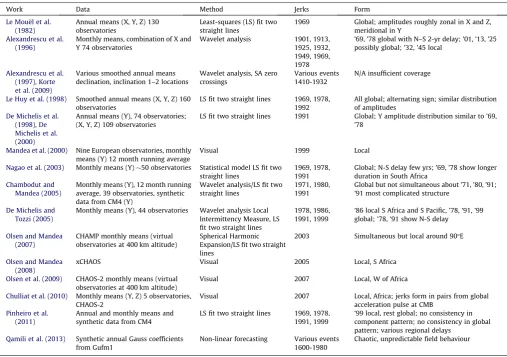
The various field derivatives in which jerks can be observed (e.g. MF, SV, SA) mean that a wide variety of detection methods can be employed. A detection method must contend with several factors, for example: noise content in the data, which may be of several ori-gins; the temporal, amplitude and spatial scales at which an event becomes significant enough to be a jerk; the proximity of consec-utive jerks; and the asynchronous form of a jerk in each field com-ponent. An overview of events detected and the various techniques used are presented inTable 1. A broader summary of studies con-cerning geomagnetic jerks can be found inMandea et al. (2010).
This study is structured in the following manner: in Section2
we introduce a two step method to remove external field noise and to identify jerks in the data; in Section3the observatory data are described and the applicability of monthly means is discussed; Section4presents the results and their subsequent interpretation before our conclusions are drawn in Section5.
2. Method
Here we describe a method comprising a combination of two primary components: the removal of external field signals from observatory monthly means after Wardinski and Holme (2011),
and the identification of jerk events in the observatory data based on the premise described byPinheiro et al. (2011). While SV can be calculated in many ways from MF data, throughout this paper SV will be calculated as the annual difference of monthly means. An-nual differences of monthly means was chosen as it reduces the great variability seen in monthly first differences allowing longer term trends to be seen without introducing the smoothing effect which results from methods involving longer period averages. An-nual differences of monthly means implies the difference between monthly time samples 12 months apart so that the SV at 6 months between the two measurements is
SVðtk6Þ ¼MFðtkÞ MFðtk12Þ; with sampling rate
D
tk¼1 month: ð1Þ
Where annual means are referenced, the SV as first differences of annual means is implied and refers to the difference between a gi-ven annual time sample and the previous sample so that the SV at 6 months between the two measurements is
SVðtk0:5Þ ¼MFðtkÞ MFðtk1Þ; with sampling rate
D
tk¼1 year: ð2Þ
2.1. External signal removal
[image:3.595.45.553.84.441.2]Externally generated magnetic signals overlap the periods at which rapid internal field variations occur and thus are a significant noise source for studies of the internal field of the Earth. Table 1
Overview of key geomagnetic jerk detection works detailing data used, detection technique and events identified (adapted fromPinheiro et al., 2011).
Work Data Method Jerks Form
Le Mouël et al. (1982)
Annual means (X, Y, Z) 130 observatories
Least-squares (LS) fit two straight lines
1969 Global; amplitudes roughly zonal in X and Z, meridional in Y
Alexandrescu et al. (1996)
Monthly means, combination of X and Y 74 observatories
Wavelet analysis 1901, 1913, 1925, 1932, 1949, 1969, 1978
’69, ’78 global with N–S 2-yr delay; ’01, ’13, ’25 possibly global; ’32, ’45 local
Alexandrescu et al. (1997), Korte et al. (2009)
Various smoothed annual means declination, inclination 1–2 locations
Wavelet analysis, SA zero crossings
Various events 1410-1932
N/A insufficient coverage
Le Huy et al. (1998) Smoothed annual means (X, Y, Z) 160
observatories
LS fit two straight lines 1969, 1978, 1992
All global; alternating sign; similar distribution of amplitudes
De Michelis et al. (1998), De Michelis et al. (2000)
Annual means (Y), 74 observatories; (X, Y, Z) 109 observatories
LS fit two straight lines 1991 Global; Y amplitude distribution similar to ’69, ’78
Mandea et al. (2000) Nine European observatories, monthly
means (Y) 12 month running average
Visual 1999 Local
Nagao et al. (2003) Monthly means (Y)50 observatories Statistical model LS fit two
straight lines
1969, 1978, 1991
Global; N-S delay few yrs; ’69, ’78 show longer duration in South Africa
Chambodut and Mandea (2005)
Monthly means (Y), 12 month running average, 39 observatories, synthetic data from CM4 (Y)
Wavelet analysis/LS fit two straight lines
1971, 1980, 1991
Global but not simultaneous about ’71, ’80, ’91; ’91 most complicated structure
De Michelis and Tozzi (2005)
Monthly means (Y), 44 observatories Wavelet analysis Local Intermittency Measure, LS fit two straight lines
1978, 1986, 1991, 1999
’86 local S Africa and S Pacific, ’78, ’91, ’99 global; ’78, ’91 show N-S delay
Olsen and Mandea (2007)
CHAMP monthly means (virtual observatories at 400 km altitude)
Spherical Harmonic Expansion/LS fit two straight lines
2003 Simultaneous but local around 90°E
Olsen and Mandea (2008)
xCHAOS Visual 2005 Local, S Africa
Olsen et al. (2009) CHAOS-2 monthly means (virtual
observatories at 400 km altitude)
Visual 2007 Local, W of Africa
Chulliat et al. (2010) Monthly means (Y, Z) 5 observatories,
CHAOS-2
Visual 2007 Local, Africa; jerks form in pairs from global acceleration pulse at CMB
Pinheiro et al. (2011)
Annual and monthly means and synthetic data from CM4
LS fit two straight lines 1969, 1978, 1991, 1999
’99 local, rest global; no consistency in component pattern; no consistency in global pattern; various regional delays
Qamili et al. (2013) Synthetic annual Gauss coefficients
from Gufm1
Non-linear forecasting Various events 1600-1980
A major source of external signals are electrical currents present in the ionosphere and magnetosphere of the Earth. Gubbins and Tomlinson (1986)used magnetic indices of external field activity as selection criteria for generating quiet time monthly means to study jerks, external signal removal from annual means via mag-netic indices was applied byDe Michelis et al. (1998, 2000)and more recentlyVerbanac et al. (2007)proposed a method of correct-ing for external signal in observatory annual means uscorrect-ing a combi-nation of field models and magnetic indices. Detailed attempts to parameterise the external field sources as part of field models are documented by e.g.Sabaka et al. (2004) and Olsen et al. (2009), allowing modelled corrections to be applied to observatory data. An alternative to the complex source parameterisations of such models is the statistical approach suggested by Wardinski and Holme (2011).
Wardinski and Holme (2011)document a method to remove SV signals which correlate with the first time derivative of a magnetic index (D_ST-index (see e.g.Mayaud, 1980)) representing primarily
the activity of the magnetospheric ring current (see e.g. Daglis et al., 1999). Alternatively, Wardinski and Holme (2011)showed that the residual between observatory data and a magnetic field model can replace theD_ST-index in their calculations as a proxy
for unmodelled external signals. Removal of such signals was shown to reduce the standard deviation of the data and thus im-prove the resolution of internal features such as jerks. A full description of the method can be found inWardinski and Holme (2011), a brief summary of which is given here.
The premise ofWardinski and Holme (2011)is that information regarding external field signals is contained in the unmodelled SV residual between observatory data and the internal magnetic field approximated by a model. Coherent signal between the residuals to the SV of the X-, Y-, and Z-components can be described by a 33 covariance matrix, assumed to be constant through time at each given observatory location. The eigenvectors of this residual covariance matrix can then be used to rotate the observed and modelled field components into the directions of least, intermedi-ate and most coherent signal; these directions will be referred to as the ‘clean’, ‘intermediate’, and ‘noisy’ field components and corre-spond to the eigenvectors with the smallest to largest magnitude eigenvalues, respectively. Wardinski and Holme (2011) showed that the noisy-component at the 50 observatories used in their
study is approximately in the North-South plane. This North-South alignment and a strong zero-lag correlation of the unmodelled residuals in the noisy-component with theD_ST-index, is consistent
with external field signals generated by the equatorial ring current. Additionally, a stronger correlation is seen between the noisy-com-ponent residuals at different observatories than to theD_ST-index,
signifying that the index does not fully explain all the unmodelled residual in the noisy-component.
It was proposed byWardinski and Holme (2011)that a zero-lag correlation based weighting function can be used to remove signal which is coherent between the noisy-component residuals at dif-ferent observatories, to produce SV time series with reduced exter-nal sigexter-nal content:
_
rcorrectedðtkÞ ¼rnoisy_ ðtkÞ
P
lC_ðtlÞrnoisy_ ðtlÞ
P
lC_ðtlÞ2
_
CðtkÞ; ð3Þ
wherer_correctedis the corrected noisy-component SV residual,r_noisyis
the noisy-component unmodelled SV residual,C_ is the noisy-com-ponent unmodelled SV residual from an alternative observatory and subscriptskandlrun over the number of time samples. This correction is applied only to the noisy-component residual before reforming the modelled and unmodelled residual component parts and rotating back to the original X-, Y-, and Z-component directions. This procedure therefore removes signal from the noisy-component residual, which when rotated back to geographic coordinates, re-sults in a removal of signal from each component based on the strength of the correlation to the external signal proxy in each component.
An advantage of this statistical approach over source parame-terisation is that it helps to account for the unpredictable nature of local induced fields, that result from heterogeneity in subsurface electrical conductivity. Local induced fields will affect the direction of the external field resulting from features such as the ring cur-rent, making their parameterisation difficult (Wardinski and Holme, 2011). As inWardinski and Holme (2011)we correct for external signal using the residual from the observatory at Niemegk (NGK), Germany, since it provides coverage of the entire timespan of interest with a well documented and reliable record (Niemegk itself is corrected using data from Chambon-la-Forêt (CLF) observatory, France). No other observatory was found to produce
1960 1970 1980 1990 2000 −20
0 20 40
dX/dt (nT/yr)
1960 1970 1980 1990 2000 20
40
dY/dt (nT/yr)
1960 1970 1980 1990 2000 10
20 30 40 50
dZ/dt (nT/yr)
Date
1960 1970 1980 1990 2000 −20
0 20
dX/dt (nT/yr)
1960 1970 1980 1990 2000 −20
0 20
dY/dt (nT/yr)
1960 1970 1980 1990 2000 −20
0 20
dZ/dt (nT/yr)
Date
[image:4.595.127.462.519.729.2])
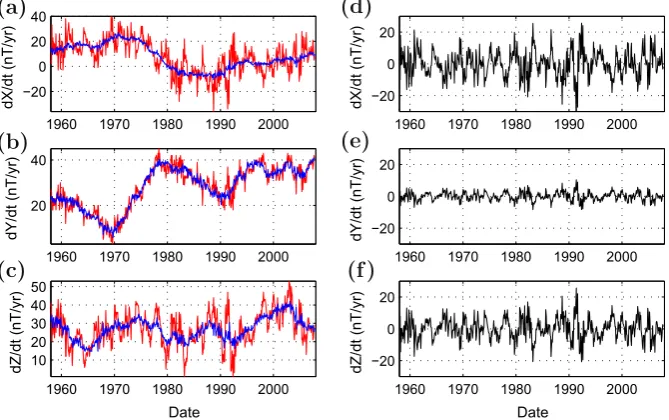
a significant improvement on the overall results, likely due to the location of Niemegk in central Europe, close to roughly 30% of the observatories used in this study. An example of the improvement made by applying the method to the data is shown inFig. 1. As expected the greatest signal variation is removed from the X- and Z-components, with limited improvement to the Y-component. The signal removed from each component can be seen to be a scaled version of the same signal, in the case ofFig. 1, the noisy-compo-nent SV residual from the relatively nearby CLF observatory. It was found that, averaged over all observatories in our study, signals with mean standard deviations of 7, 2 and 5 nT/yr were removed from the X-, Y- and Z-components, respectively. The mean peak-to-peak amplitude ranges of these removed signals were 59, 13 and 41 nT/yr for the X-, Y- and Z-components, respectively.
2.2. Jerk identification
Pinheiro et al. (2011) described a method for applying a two-part linear regression to the SV of observatory annual means, generating a probability density function (PDF) of the likeliness of
potential jerk occurrence times. A window of a single component of SV data were selected and the two-part linear regression iter-ated across the window, considering a potential jerk occurrence at each time step of 0:001yrs. At each time step, the misfit of the regression to the data was calculated and converted to a probabil-ity value to build up the PDF by:
PDFðt0Þ /exp
v
2ðt0ÞðN3Þ 2v2
min
; ð4Þ
where t0 is the proposed jerk occurrence time,
v
2 is theleast-squares misfit with a minimum value for the window of
v
2 min, andNis the number of data points in the window.
Assuming Gaussian error distributions about the peaks in like-liness, estimates of the uncertainties in these occurrence times and in jerk amplitudes were calculated.Pinheiro et al. (2011) ap-plied this procedure to selected 11–15 year time windows of data roughly centred about the previously identified jerk occurrences of 1969, 1978, 1991 and 1999 in the X-, Y- and Z-components of 123 observatories worldwide.
Possible events were considered an identified jerk if the PDF function in the time window allowed a 68% confidence window (1 standard deviation) to be defined about the most likely occur-rence time. Other potential jerks were excluded if a peak in likeli-ness was seen but the confidence interval could not be contained in the window chosen. If no peak likeliness was seen in occurrence time in the window, no jerk was identified.
2.2.1. Sliding window regression
We propose that the use of a static window of data may bias the identification by severely limiting the extent and time of potential jerk events considered. Methods which utilise complete time series rather than requiringa prioridata selection (e.g.Stewart and Wha-ler, 1995; Alexandrescu et al., 1996; De Michelis and Tozzi, 2005) can be seen as more robust in this respect. We thus propose a slid-ing window, actslid-ing as described byPinheiro et al. (2011), but with the window shifting, one time step per iteration, along the series being considered and the PDF calculation repeated. A summation of the resulting overlapping functions produced can then be nor-malised (to an integral of 1) to give a continuous PDF for the entire series which has considered each possible jerk time at every rela-tive time in a window (Fig. 2). This removes the bias towards events centred in the window and also removes any potential bias arising from manually selected window times.
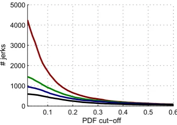
The time uncertainty estimation procedure of Pinheiro et al. (2011)(uncertainties are taken to be1 standard deviation of each PDF peak, assumed to be Gaussian) can still be applied to peaks in the PDF but we introduce the addition of a threshold probability above which events are deemed significantly likely compared to the background level of likeliness which results from the misfit to the variability in the data. A threshold of 0.2 was chosen based on a trade-off curve of the number of jerks identified versus the probability threshold (Fig. 3). This threshold assumes that the rel-atively high peaks in the jerk time PDFs are the most sound esti-mates of jerk times and was set slightly to the right of the knee of the trade-off curve (Fig. 3) to reduce the likelihood of false positives.
This method moves towards identification of jerk-like trends in SV with minimala prioriinformation required; nevertheless some assumptions are made and limiting parameters imposed to counter the issues of the jerk identification problem. It is assumed that: a jerk takes the form of an instantaneous change in the gradient of SV (a step in SA); that there is a minimum jerk amplitude below which events are not considered likely to be jerks; and that the misfit of the jerk model to the data can be related to the probability
1960 1970 1980 1990 2000 −10
0 10 20 30 40
dZ/dt (nT/yr)
1960 1970 1980 1990 2000 0
0.1 0.2
Date
[image:5.595.68.269.68.253.2]Fig. 2.Example of jerk identification using the sliding window method for the
Z-component of SV (a) at Chambon-la-Forêt (CLF), France. PDF function (b) used to identify the most likely jerk times, marked by positive (red) and negative (black) time uncertainties. Jerks are judged to be distinct peaks in the PDF above the cut off value (green line). (For interpretation of the references to colour in this figure legend, the reader is referred to the web version of this article.)
0.1 0.2 0.3 0.4 0.5 0.6 0
1000 2000 3000 4000 5000
PDF cut−off
# jerks
[image:5.595.77.259.344.472.2]of that model representing the data by Eq.(4)both for sections of data in which jerks are present or absent.
In addition to the threshold probability mentioned previously, a magnitude of 3 nT/yr2was chosen as the minimum jerk amplitude
which is recognised as a significant trend above the variability of the background noise level in the data. Since it is not assumed that a jerk is present in each window, this limit is required to impose zero probability on features such as long linear sections of data, which otherwise show a low misfit when both sections of the lin-ear regression align approximately parallel to each other. Ampli-tude best estimates are taken to be the value which produces the lowest misfit to the data when considering the range of amplitude estimates from all time windows which identify a given time as a potential jerk. The uncertainties on amplitude estimates are then calculated as the differences between the best estimate and the
maximum and minimum values of the range of amplitude estimates.
The length of the time window in which data is considered dur-ing each linear regression must also be imposed. It was decided to utilise a variety of window lengths as a reassurance of the robust-ness of identified events due to the limiting role the window length plays in the resolution of consecutive events. Consecutive jerks which occur within a single window length are less likely to be re-solved individually. Thus jerks were identified with window lengths of 5, 10, 15 and 20 yrs. The time step occurrences at which possible events are considered must be defined, this was chosen to be 0.001 yr as used byPinheiro et al. (2011)since this sampling rate is sufficiently higher than the monthly (0.08yr) data sampling and produces smooth PDFs. All input parameter values were cho-sen after testing using both synthetic and real data.
−90° 0° 90°
−90° −45° 0°
45° 90°
1960 1970 1980 1990 2000 25
50 75 100
Date
[image:6.595.112.476.74.171.2]# observatories
Fig. 4.Map showing observatory locations used in this study (a). The 8 groups of symbols show regions of observatories as described in Section4. While all the observatories highlighted above were used in this study, not all were operating throughout the entire period of interest, (b) shows the number of observatories operating in any given six month period between 1957 and 2008. The number of observatories providing minimum length time series of 5 yrs (red), 10 yrs (green), 15 yrs (blue) and 20 yrs (black) are shown. (For interpretation of the references to colour in this figure legend, the reader is referred to the web version of this article.)
1960 1980 2000 0
10 20 30
#
Jerks
1960 1980 2000 0
10 20 30
Date
Weighting max 94 stns
1960 1980 2000 0
10 20 30
1960 1980 2000 0
10 20 30
Date
1960 1980 2000 0
10 20 30
1960 1980 2000 0
10 20 30
Date
1960 1980 2000 0
10 20 30
1960 1980 2000 0
10 20 30
Date 1960 1980 2000
0 20 40 60 80
All components
#
Jerks
1960 1980 2000 0
20 40 60 80
X
1960 1980 2000 0
20 40 60 80
Y
1960 1980 2000 0
20 40 60 80
Z
Fig. 5.Histograms of detected jerks in 12-month time bins between 1957 and 2008, (a) shows straight counts when results from 5-, 10-, 15- and 20-yr windows are
[image:6.595.124.460.243.520.2]This method thus provides a means of consistently identifying features which statistically fit the definition of a jerk in the SV. It is also able to provide a relative probabilistic weighting with which to consider the identified events as constrained by the data, and a quantitative estimate of the uncertainties in times and in jerk amplitudes.
3. Data
Monthly mean MF data were obtained from the Bureau Central de Magnétisme Terrestre (BCMT), World Monthly Means Database Project. This database comprises full monthly averages of all hourly mean values for the X-, Y-, and Z-components at 118 observatories worldwide and was compiled byChulliat and Telali (2007)from hourly means, initially obtained from the World Data Centre (WDC) for Geomagnetism at the British Geological Survey, Edin-burgh. Further to the consistency checks of Chulliat and Telali (2007), we have applied all documented baseline corrections and accounted for gaps of unrecorded data in one of two ways. Gaps shorter than 6 months were interpolated using a linear fit to the field component in question. A minimum of 12 months of data either side of a gap was required for interpolation to be performed. For gaps longer than 6 months the records were split into separate time series on either side of the gap and will be considered as indi-vidual records from here on.
When considering analysis of observatory data it is important to consider the dependence of any interpretation on the spatial and temporal distribution of the data upon which it is founded. It is well known that observatory data provide spatial sampling biased heavily towards continental regions, particularly Europe and North America, and that the density of observations varies through time, generally increasing towards the present day as more observato-ries have been established (seeFig. 4).
The procedure described in detail in Section2.1requires use of a magnetic field model. For this purpose C3FM2 ofWardinski and Lesur (2012)was used. The model is a fit to observatory SV over the period of 1957.0–2008.4, further constrained by satellite field models in 1980 and 2004. As such it provides coverage specifically tailored to SV across the period in which observatory data is most widely available. The data timespan of this study was thus con-strained by the model length. While observatory data are available extending back to the late 1800s, the spatial coverage is too limited for our study. While C3FM2 was chosen for this study, the methods
described in Section2are, in principle, applicable to any period for which observations and models are available.
3.1. Data sampling
We suggest that when investigating rapid, sharp features such as jerks it is preferable to utilise monthly sampling of observatory
1960 1980 2000 0
5 10 15
#
Jerks
1960 1980 2000 0
5 10 15
Date
Weighting
m
ax
21
stns
1960 1980 2000 0
5 10 15
1960 1980 2000 0
5 10 15
Date
1960 1980 2000 0
5 10 15
1960 1980 2000 0
5 10 15
Date
1960 1980 2000 0
5 10 15
1960 1980 2000 0
5 10 15
Date 1960 1980 2000
0 10 20 30
All components
#
Jerks
1960 1980 2000 0
10 20 30
Weighting
max
73
stns
1960 1980 2000 0
10 20 30
X
1960 1980 2000 0
10 20 30
1960 1980 2000 0
10 20 30
Y
1960 1980 2000 0
10 20 30
1960 1980 2000 0
10 20 30
Z
1960 1980 2000 0
[image:7.595.137.471.69.449.2]10 20 30
data with as little smoothing as possible to achieve the best time resolution. Annual mean observatory data were used byPinheiro et al. (2011)in preference to monthly means due to the greater availability of stations and the view that monthly means, in the form of 12 month running means of first differences in dipole coor-dinates (X- and Y-components rotated to be parallel and perpen-dicular to the dipole axis), contain correlated external noise as well as much greater variability. The correlated external signal in this case breaks the assumption of Gaussian error distributions and the high variability leads to unacceptable misfit of linear trends to the data. It was also noted byPinheiro et al. (2011)that jerks appeared to be more contemporaneous between field compo-nents when considering annual means.
We find that spatial coverage of observatory data, while gener-ally poor, is not greatly reduced by considering monthly means over annual means. In this study 96 observatories were used when considering an 11- to 15-yr window length as used byPinheiro et al. (2011)who utilised 123. Of the 27 additional stations used byPinheiro et al. (2011), the majority are short Northern hemi-sphere records in the late 20th to early 21st century and do not greatly influence the spatial or temporal distributions of data used. For window lengths of 5 yrs, 103 observatory locations were found to be suitable whilst for windows of 20 yrs, 76 observatory records were available.
The assumption that monthly means contain too much corre-lated signal which is not present in annual means (Pinheiro et al., 2011) is best addressed via an example. Considering the observa-tory record from Niemegk (NGK), Germany, during the period of the C3FM model, the 3
3 covariance matrix (Dannual) of annual
means unmodelled SV residuals (X-, Y-, Z-components) and its cor-responding normalised eigenvectors (
v
) and eigenvalues (k) are found to be (to one decimal place)Dannual¼
17:2 5:5 14:7
5:5 2:1 4:0
14:7 4:0 28:7 2
6 4
3
7 5ðnT=yrÞ
2
;
v
clean¼0:4 0:9 0:0 2
6 4
3
7
5;kclean¼0:3ðnT=yrÞ 2
;
v
intermediate¼0:8 0:3
0:6 2
6 4
3
7
5;kintermediate¼7:9ðnT=yrÞ 2
;
v
noisy¼0:6 0:2 0:8 2
6 4
3
7
5;knoisy¼39:8ðnT=yrÞ 2
;
ð5Þ
while for monthly means unmodelled SV residuals the covariance matrix (Dmonthly), eigenvectors and eigenvalues are found to be
Dmonthly¼
79:8 25:5 58:0
25:5 10:0 18:0
58:0 18:0 66:4 2
6 4
3
7 5ðnT=yrÞ
2
;
v
clean¼0:3 0:9 0:0 2
6 4
3
7
5;kclean¼1:6ðnT=yrÞ 2
;
v
intermediate¼0:6 0:2
0:8 2
6 4
3
7
5;kintermediate¼15:6ðnT=yrÞ 2
;
v
noisy¼0:7 0:2 0:6 2
6 4
3
7
5;knoisy¼139:0ðnT=yrÞ 2
:
ð6Þ
The covariance matrices describe the coherency of signal between the X-, Y-, and Z-components and have associated eigenvectors and eigenvalues which describe, respectively, the directions and magnitudes of these signals. Comparing Eqs.(5) and (6)it can be seen that the eigenvalues are of greater magnitude and thus the coherency of signal is greater for monthly means while the eigen-vectors are in similar directions for both annual and monthly data. This shows that while reduced in magnitude, the coherent signal is not removed by calculating annual means. As expected, the reduced covariance seen with annual means is only from the reduction in variability of the signal overall. These two cases can be compared to the covariance matrix (Dcorrected monthly), eigenvectors and
eigen-values of monthly means unmodelled residuals once external signal is accounted for as described in Section2
Dcorrected monthly¼
2:0 0:2 2:6
0:2 2:6 1:4
2:6 1:4 3:7
2
6 4
3
7 5ðnT=yrÞ
2
;
v
clean¼0:7 0:3 0:6 2
6 4
3
7
5;kclean¼ 0:1ðnT=yrÞ 2
;
v
intermediate¼0:4 0:9 0:1 2
6 4
3
7
5;kintermediate¼2:3ðnT=yrÞ 2
;
v
noisy¼0:5
0:3 0:8 2
6 4
3
7
5;knoisy¼6:0ðnT=yrÞ 2
:
ð7Þ
It is clear that there is much improvement with the removal of coherent unmodelled signal: smaller eigenvalues imply less coher-ent signal than for untreated annual or monthly data. The eigenvec-tors, the direction of the dominant coherent signal, are also altered and no longer show the same contaminating ring current effects with the cleanest component direction now close to that of the ori-ginal noisy component. With little covariance between the field components, the assumption of Gaussian errors made byPinheiro et al. (2011)can hold for monthly data, making them suitable for this study. The denser sampling leads to greater accuracy in time identification of jerks since the process of calculating annual means from monthly means introduces a smoothing to the data, rounding off the sharp features of jerks to create a broader apex in the SV.
4. Results
Due to the large amount of data involved and the wide extent of results generated, only the key results are summarised here. The full results of the identified jerks from this study are available in theSupplementary material. This resource includes data files con-taining all identified jerk times with associated properties such as uncertainties, probabilities and jerk amplitudes as well as addi-tional figures and movies of jerk identifications through time.
20-yr window in all components. These values nevertheless show that the use of monthly mean data has indeed increased the time resolution of jerk events compared to previous studies (mean uncertainties of 1.4 yrs were found by Pinheiro et al. (2011)). The positive and negative uncertainties were found to be symmet-rical and therefore consistent with the assumption of Gaussian er-ror distributions. The uncertainty estimates were also found to be approximately constant through the time period studied. The mean uncertainty estimates of jerk amplitudes were found to be on the order of2:1 nT/yr2. As noted byPinheiro et al. (2011)jerk
amplitudes are a robust measure with the sign of contemporary jerk amplitudes at nearby observatories seen to be consistent.
4.1. Temporal distribution
The timing of jerks is here assessed by histograms of occur-rences through time for a variety of spatial regions to assess the robustness of the idea of specific global or local events. A series of straight histogram counts and of equivalent weighted histo-grams were calculated. The weighted count (Eq.(8)) is calculated as the number of identified jerks in a time bin (ndetections) multiplied
by the ratio of the number of active observatories in a given time bin (obsactive) to the maximum number of observatory locations
in the study (obstotal):
Wbin¼ndetectionsobsactive
obstotal: ð
8Þ
Whilst it may seem contradictory to down-weight the significance of high proportions of detections at low numbers of active observa-tories, the weighting is designed to favour observations at the great-est number of observatories to assess whether identifying global events is a justified conclusion. The uncertainty in the time
occurrence of each identified event is assumed to be inconsequen-tial for the histograms provided the time bins are wider than the magnitude of the uncertainty estimates, thus a minimum bin width of 12 months is used.
Since the different window lengths used in the identification procedure favourably resolve features at different timescales, a combined histogram of results from all window lengths is shown (Fig. 5a). This was used to identify the periods of most frequent jerk activity. Relative peaks can be seen in 1968–71, 1973–74, 1977–79, 1983–85, 1989–93, 1995–98 and 2002–03 with additional sugges-tions of events in the early 1960s and the late 2000s. These periods fall at the ends of the data set and thus suffer a lack of resolution from edge effects of the identification procedure. Additionally, the early 1960s are poorly resolved spatially due to this period having the lowest coverage of observatories in this study. The his-tograms inFigs. 5–8show that in general the proportion of obser-vatories at which events are identified at a given time is low. Considering all components at all observatories included in the study worldwide, the most widespread jerk identified is seen in 1989–93 at30% of the observatories (Fig. 5b). The predominant peaks in the global histogram (Fig. 5a, combined component histo-gram) represent both a combination of events from all field compo-nents e.g. in the 1990s, and also exceptionally high counts from a single component e.g. 1977–79 in the Y-component. These peaks can also be the result of contributions from various regions at over-lapping times to produce a peak in the global histogram. When only observatories which are located in the Northern or Southern Hemisphere are considered (Fig. 6) it can be seen that events in the Northern Hemisphere dominate the global distribution due to the contribution from 73 observatories compared to 21. While the Northern Hemisphere (and thus global) results can in places be described as showing individual peaks of high numbers of jerks
1960 1980 2000 0
2 4
Date
Weighting
max
4
stns
1960 1980 2000 0
2 4
Date
1960 1980 2000 0
2 4
Date
1960 1980 2000 0
2 4
Date 1960 1980 2000
0 10 20
Weighting
max
27
stns
1960 1980 2000 0
10 20
1960 1980 2000 0
10 20
1960 1980 2000 0
10 20 1960 1980 2000
0 2 4 6 8
Weighting
max
9
stns
1960 1980 2000 0
2 4 6 8
1960 1980 2000 0
2 4 6 8
1960 1980 2000 0
2 4 6 8 1960 1980 2000
0 10 20
All components
Weighting
max
29
stns
1960 1980 2000 0
10 20
X
1960 1980 2000 0
10 20
Y
1960 1980 2000 0
10 20
[image:9.595.130.475.67.392.2]Z
detected in a short period of time, the Southern Hemisphere results do not mirror this pattern. This is potentially due to the lack of data rather than the absence of events. A point of interest is that a peak is seen around 1968-1971 in both hemispheres which does appear to fit the reported observation of an event occurring in the North-ern Hemisphere 1–3 yrs before the SouthNorth-ern Hemisphere ( Alex-andrescu et al., 1996). This trend of short North-South delay is not seen for any other distinct peaks and does not appear to be a consistent feature of jerks although the events in 1989–93 and 1995–98 are observed to be largely hemispheric. It is likely that these periods represent two or more regional events overlapping in time, a common feature of the peaks in the global histograms.
The global time distribution of jerks can be broken down further into jerks occurring in spatially distinct regions of observatories (shown onFig. 4a). The regional histograms for observatories in Europe, Africa, North America and South America (Fig. 7)and Asia, Australasia, the Southern Indian Ocean and the Pacific Ocean (Fig. 8) show which particular components in which regions con-tribute to the globally observed trends. For example, the distinct global peak around 1969 is predominantly a feature of the X-and Y-components in Europe, the only other significant contribu-tions coming from the Y-components in North America and Asia. We find the event to be very poorly constrained in the Southern Hemisphere.
The global peak around 2003 (Fig. 5a) appears only weakly in the results for the 10-yr window (Figs. 5(b) 6,7,8), due to the short timescale of the features in the SV post 2000 and the proximity to the end of the data set. As such, detections are limited with win-dows of 10-yrs and longer but frequent with the 5-yr window. Proximity to the end of the data set is likely also the reason we do not resolve the 2005 (Olsen and Mandea, 2008) and 2007 (Olsen
et al., 2009; Chulliat et al., 2010) events. Visual inspection of time-series suggests that events on a similar scale to those post 2000 may also occur in the early 1960s, producing small peaks in the histograms (Fig. 5). These time periods may benefit from a more fo-cused study.
The 1990s show a high incidence of identified events across all regions, focused in the Y- and Z-components in the Northern Hemisphere in 1989–93 and the X- and Z-components in the Southern Hemisphere in 1995–98. These periods may host several events, the overlapping durations of which prevent the definition of a sharp peak. The focus of the latter of these two peaks in the poorly sampled Southern Hemisphere may explain the previous uncertainty over the extent of the mooted 1999 jerk (De Michelis and Tozzi, 2005; Pinheiro et al., 2011).
Further distinct events are difficult to trace between regions, being detected in various components in various regions with the dominant signal coming from European observatories.
4.2. Spatial distribution and morphology
Despite the fact that generally only a small proportion of obser-vatories identify jerks in a given time period, it is still informative to look at the spatial distributions of these events. As noted by
Pinheiro et al. (2011), the jerk amplitudes prove to be a reliable measure, showing that even where low probability events are identified, the uncertainty estimates are small and the amplitudes of events detected at observatories in close proximity show the same polarity and similar magnitude.
Examples of the amplitude distributions for three characteristi-cally different regions of peaks in the histograms seen in Section4.1
are depicted here: a well documented global peak whose precise
1960 1980 2000 0
1 2 3
Date
Weighting
max
3
stns
1960 1980 2000 0
1 2 3
Date
1960 1980 2000 0
1 2 3
Date
1960 1980 2000 0
1 2 3
Date 1960 1980 2000
0 1 2 3
Weighting
max
3
stns
1960 1980 2000 0
1 2 3
1960 1980 2000 0
1 2 3
1960 1980 2000 0
1 2 3 1960 1980 2000
0 2 4 6 8
Weighting
max
9
stns
1960 1980 2000 0
2 4 6 8
1960 1980 2000 0
2 4 6 8
1960 1980 2000 0
2 4 6 8 1960 1980 2000
0 5 10
All components
Weighting
max
10
stns
1960 1980 2000 0
5 10
X
1960 1980 2000 0
5 10
Y
1960 1980 2000 0
5 10
[image:10.595.118.465.66.397.2]Z
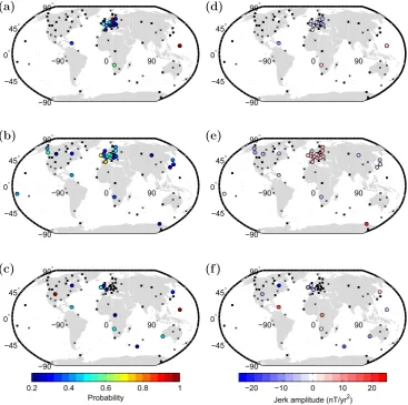
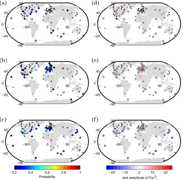
occurrence time varies by region (1968–71, Fig. 9); a broad period of the highest incidence of events in all components in all regions (1989–93,Fig. 10); and a period which contains an event whose extent is debated between various studies (1995–98,
Fig. 11). For equivalent figures of the remaining periods of relative peaks in jerk occurrences, we refer the reader to the Supplemen-tary material.
The jerk amplitudes of 1968–71 (Fig. 9) are seen to be domi-nated by Northern Hemisphere, particularly European, observa-tions in the X- and Y-components. The X- and Y-components show similar spatial and magnitude patterns but with opposite polarity. There is no evidence of the zonal patterns in X- and Z-components or the sectoral pattern in the Y-component as de-scribed by early works such asLe Mouël et al. (1982). The Z-com-ponent is largely unconstrained over Europe and a much less significant event than those in the X- and Y-components. Our amplitude results fit well with those calculated for the 1969 jerk by Le Huy et al. (1998), De Michelis et al. (2000) and Pinheiro et al. (2011)and disagree with those ofLe Mouël et al. (1982)in so doing. Little can be determined conclusively about the morphol-ogy in the Southern Hemisphere.
The jerk amplitudes in the period of 1989–93 (Fig. 10) show a different style from those of 1968–71. Jerks are seen more consis-tently across wider regions in all three components. There is a very high incidence of jerks in all three components at overlapping
times during the 5-yr period of 1989–93. Twin peaks of 1–3 yrs in jerk occurrences are seen in the X-, Y- and Z-components in an asynchronous manner, leading to an overall peak spanning 1989–93 (Figs. 5–8). The resulting pattern of amplitudes is more complicated than that of 1968–71, with localised variations in polarity. The jerks in the Y-component in Europe appear to transi-tion from positive to negative polarity through time while the X-and Z-component occurrences peak twice with the same polarity. Observations in X- and Y-components in North America appear to transition between positive and negative amplitudes spatially with all jerks occurring in a single span of 2–3 yrs. Our results sug-gest the complicated structure and varying descriptions of the re-ported 1991 jerk (seeLe Huy et al., 1998; Chambodut and Mandea, 2005; De Michelis and Tozzi, 2005) can be explained by a double peak in the occurrences of jerks in our results in the period of 1989–93. Our amplitude results from the latter half of the 1989– 93 peak best agree with the 1991 jerk amplitudes ofLe Huy et al. (1998), De Michelis et al. (2000) and Pinheiro et al. (2011).
Jerk amplitudes in the period of 1995–98 (Fig. 11) are unusual with respect to other periods of frequent jerk occurrences in that most of our detections are in the Southern Hemisphere. Our ampli-tude results are consistent with those ofMandea et al. (2000), De Michelis and Tozzi (2005)but not those ofPinheiro et al. (2011). We find minimal evidence of jerks in Europe, and more widespread occurrences in the rest of the world whilst Pinheiro et al., 2011
−90° 0° 90°
−90° −45° 0°
45° 90°
−90° 0° 90°
−90° −45° 0°
45° 90°
−90° 0° 90°
−90° −45° 0°
45° 90°
Probability
0.2 0.4 0.6 0.8 1
−90° 0° 90°
−90° −45° 0°
45° 90°
−90° 0° 90°
−90° −45° 0°
45° 90°
−90° 0° 90°
−90° −45° 0°
45° 90°
[image:11.595.119.487.67.432.2]Jerk amplitude (nT/yr2) −20 −10 0 10 20
found very limited local evidence, largely in Europe. This discrep-ancy may be a result of the limited data window of 11–15 yrs of annual means selected byPinheiro et al. (2011)which was centred around 1999 and thus possible overlap of events in the early to mid 1990s and 2000s, which we define as temporally close but distinct periods of frequent jerk occurrences.
A peak in the occurrences of jerks is seen in the period of 1977– 79 (Figs. 5–8), comparable to the 1978 jerk and corresponding amplitudes observed byDe Michelis et al. (1998), Le Huy et al. (1998) and Pinheiro et al. (2011)in all components. The observa-tions of this period bear much similarity to those of 1968–71 including providing few constraints of events in the Southern hemisphere.
The jerks in the period of 2002–03 (Fig. 5a andSupplement) are seen in all three components. As mentioned in Section4.1, the proximity to the end of the data set means that few events are seen with a window of 10 yrs or longer and jerks are more readily iden-tified with the 5-yr window. A unique characteristic of this time period is that all the observations of the Z-component suggest a strong hemispheric dichotomy in polarity (seeSupplement), a fea-ture not seen in any other period investigated. Our amplitude re-sults here agree with the observations of Olsen and Mandea (2007)in all three components.
The reported 2005 (Olsen and Mandea, 2008) and 2007 (Olsen et al., 2009; Chulliat et al., 2010) jerks are not prominent in our re-sults; this is likely due to the reduced effectiveness of our identifi-cation method with proximity to the end of the data set. Observed
amplitude patterns do not appear to be consistent in form between events although regional polarity does seem to show an alternating pattern. This will be discussed in Section4.4.
4.3. Spatiotemporal relationship
The relationship between the temporal and spatial patterns of jerk occurrences could hold information as to their source mecha-nism. For example jerks generated by torsional oscillations (e.g.
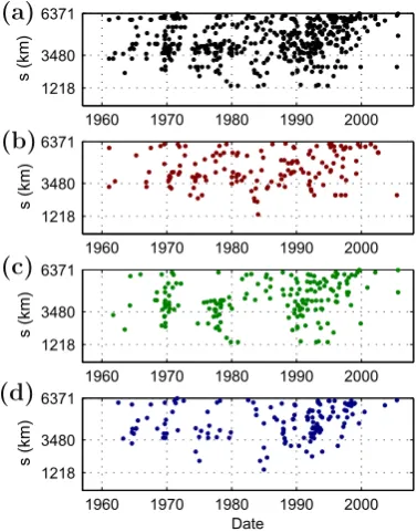
Bloxham et al., 2002) may show evidence of wave propagation in the cylindrically radial direction. The presence of trends in identi-fied jerk times with cylindrical radius (or latitude) and longitude were investigated. No clear relationships were found in any combi-nation of these variables. It was found that accounting for the con-centration of observatory locations in certain regions, jerk times appear to be distributed evenly through latitude, longitude or cylindrical radius and concentrated only about certain time periods asFigs. 5–8show. It can be seen inFig. 12that while some epochs, e.g. around 1970 in the Y-component, show a more dense cluster-ing in time of jerks at a range of cylindrical radii, there is no con-sistent pattern between the events which correspond to relative peaks in the histograms inFigs. 5–8.
4.4. Periodicity of jerk amplitude
It has been observed (e.g.Le Huy et al., 1998; Chulliat et al., 2010) that the series of jerks at approximately 1969, 1978 and
−90° 0° 90°
−90° −45° 0°
45° 90°
−90° 0° 90°
−90° −45° 0°
45° 90°
−90° 0° 90°
−90° −45° 0°
45° 90°
Probability
0.2 0.4 0.6 0.8 1
−90° 0° 90°
−90° −45° 0°
45° 90°
−90° 0° 90°
−90° −45° 0°
45° 90°
−90° 0° 90°
−90° −45° 0°
45° 90°
[image:12.595.109.480.67.432.2]Jerk amplitude (nT/yr2) −20 −10 0 10 20
1991 show a trend of alternating polarity of jerk amplitude. It has been suggested this is a feature of long term memory in the source mechanism of jerks (e.g.Alexandrescu et al., 1996; Le Huy et al., 1998). With regard to analysing this trend in our results three questions arise: are successive jerks seen to change amplitude polarity through time? Is this trend zero mean? Is this polarity change periodic? The amplitude maps inFigs. 9–11show that at a given time the polarity of the jerk amplitude varies across the globe thus we consider the trends in smaller regions of observato-ries where the same polarity signal would be expected. We focus on Europe and North America since these two regions provide the greatest coverage both in terms of numbers of observatories (29 and 27, respectively) and time spans of data.
We find that for both Europe and North America, in all three components, the jerk amplitude polarity can be seen to vary through time (Figs. 13(a–c) and14(a–c)). In both regions, for all components these variations are zero mean to within a tolerance of 1 nT/yr2 although distinct clustering of events in time and
amplitude is stronger in Europe than in North America as the his-tograms inFig. 7(a and c) show.
To assess the possible periodicity in jerk amplitudes we esti-mate the power spectra of the jerk amplitudes via the Lomb-Scar-gle method of least-squares spectral analysis (see Lomb, 1976; Scargle, 1982). It can be seen (Figs. 13(d–f) and 14(d–f)) that there are predominant peaks in the spectra, which synthetic testing indi-cates are not artefacts of the irregular time sampling of the jerk amplitudes. The statistical significance (a) of peaks in the spectra
−90° 0° 90°
−90° −45° 0°
45° 90°
−90° 0° 90°
−90° −45° 0°
45° 90°
−90° 0° 90°
−90° −45° 0°
45° 90°
Probability
0.2 0.4 0.6 0.8 1
−90° 0° 90°
−90° −45° 0°
45° 90°
−90° 0° 90°
−90° −45° 0°
45° 90°
−90° 0° 90°
−90° −45° 0°
45° 90°
[image:13.595.119.488.68.431.2]Jerk amplitude (nT/yr2) −20 −10 0 10 20
Fig. 11.AsFig. 9but for the period of 1995–1998.
1960 1970 1980 1990 2000 1218
3480 6371
s (km)
1960 1970 1980 1990 2000 1218
3480 6371
s (km)
1960 1970 1980 1990 2000 1218
3480 6371
s (km)
1960 1970 1980 1990 2000 1218
3480 6371
s (km)
Date
Fig. 12.All identified jerk occurrences using a 10-yr window plotted against
[image:13.595.74.263.470.711.2]is judged as a function of power derived from the exponential probability distribution of the spectrum, the number of frequencies tested and the oversampling factor (seePress et al., 2007). Thus higher power and lower values of
a
represent more certain results. Generally the spectra for Europe were found to hold more signifi-cant peaks than those for North America. It is possible that the length of the identification window used to calculate the linear regression creates artifacts in the periodicity of the identified jerk events. While no spectral peaks appear at aliased window periods, only signals which appear consistently in results from the 5-, 10-, 15- and 20-yr windows are considered robust observations.European observatories were found to show significant, consis-tent signals for all detection window lengths at periods of18– 20 yrs in the Y-component. Significant signals for three of the four window lengths were seen at17–20 yrs in the X-component,7– 8 yrs in the Y-component, and 7 yrs and15–16 yrs in the Z-component. North American observatories were not found to show
consistent signals at all detection window lengths but moderately significant signals were seen for three of four window lengths at
11–12 yrs and19–21 yrs in the Y-component and18–22 yrs in the Z-component. The greater uncertainty of results for North America may be attributed to the greater spatial extent of the observatories (and thus greater variation of signal) compared to the dense network in Europe.
With the limited data available it is hard to be conclusive as to the presence of periodic signals worldwide. However, the premise is an interesting one, perhaps complementary to the6-yr mag-netic and LOD signals (or higher harmonics of) reported byGillet et al. (2010), Silva et al. (2012) and Abarco del Rio et al. (2000). Periodicity in the polarity of jerk amplitudes implies that the ob-served step changes in the SA associated with jerks regularly oscil-late between a similar maximum and minimum magnitude. This suggests that the source mechanism for the jerk signal is periodic and shows a relatively consistent magnitude effect in the observed
1960 1970 1980 1990 2000 −10
0 10
A
(nT/yr
2)
1960 1970 1980 1990 2000 −20
0 20
A
(nT/yr
2)
1960 1970 1980 1990 2000 −20
0 20
Date
A
(nT/yr
2)
0 10 20 30 40 50
0 20 40
α=0.001
Power
0 10 20 30 40 50
0 20 40
α=0.001
Power
0 10 20 30 40 50
0 20 40
α=0.001
Power
[image:14.595.108.477.69.274.2]Period (yrs)
Fig. 13.Time series of jerk amplitudes for all European observatories (a–c) and corresponding power spectra calculated as Lomb-Scargle periodograms (d–f). Plot rows show X-, Y- and Z-components from top to bottom. Symbolarepresents the statistical certainty level as a function of power with higher power more certain. Jerks were detected using the 10-yr window. The highlighted periods in (d–f) are plotted as least-square fit sinusoids over the data in (a–c).
1960 1970 1980 1990 2000 −20
0 20
A
(nT/yr
2 )
1960 1970 1980 1990 2000 −20
0 20
A
(nT/yr
2 )
1960 1970 1980 1990 2000 −50
0 50
Date
A
(nT/yr
2 )
0 10 20 30 40 50
0 5 10 15
α=0.01
α=0.1
α=0.5
Power
0 10 20 30 40 50
0 5 10 15
α=0.01
α=0.1
α=0.5
Power
0 10 20 30 40 50
0 5 10 15
α=0.01 α=0.1
α=0.5
Power
Period (yrs)
[image:14.595.109.480.333.540.2]magnetic field in a given region. It has yet to be determined if the disparities in the periodicity observed between European and North American observatories persist to the core mantle boundary as a feature of the source mechanism or are an effect resulting from interaction with a conducting mantle (e.g.Pinheiro and Jackson, 2008).
5. Conclusions
The jerk identification method developed here proves to be a useful tool in the assessment of geomagnetic jerks in observatory data. Applying our specified detection criteria, requiring minimal
a prioriinformation, leads to the robust identification of all events
which exhibit the characteristic form of a jerk in the SV. The tech-nique also allows the variation of the selection criteria to assess the effects of the scale and definition of a jerk that is imposed. Using monthly mean data and removing external field signals produces increased time resolution and reduced uncertainty estimates on jerk occurrence times and amplitudes compared to the results of
Pinheiro et al. (2011). Combined with relative probabilities for each event identified, the method provides a means to temper the cer-tainty of each observation to assess how well our observations are constrained by the data.
The results presented here suggest that the established global and local jerk times reported in previous studies do not fully char-acterise the observations as a whole but rather describe select por-tions of a much larger data set. It should be noted that observatory data provide a very sparse data set for even the best observed events and that this should be taken into consideration when assessing the potential occurrence of global events. Nevertheless our observations suggest that between the epochs of 1957 and 2008 there are periods when jerks occur more frequently in
partic-ular regions of the world (Fig. 15). These can be summarised as 1968–71, 1973–74, 1977–79, 1983–85, 1989–93, 1995–98 and 2002–03 with the suggestion of further poorly sampled events in the early 1960s and late 2000s. It should be noted that none of these events were detected at more than 30% of observatories in a given year. These peaks in jerk occurrences do not appear to manifest as consistent forms in the distribution of amplitudes and are seen to occur in various combinations of components. Jerks are not seen to occur simultaneously across all regions of the globe and the bias of the data set to the Northern Hemisphere, particu-larly Europe, is evident in the composition of global jerk occur-rences. Neither do jerks show a consistent relationship in patterns of occurrence between regions, which suggests that the relationship between so called jerk delay times and properties such as mantle electrical conductivity do not follow a simple or constant rule if at all. Better understanding of the cause of jerks may be needed to explain the variations in occurrence times observed.
Our results suggest that previously reported observations of jerks are largely consistent with our findings but restricted to those events of greatest magnitude and isolation in time. We show that event occurrences are frequent and occurrence patterns vary but that there are times when many events are seen in several compo-nents across large portions of the Earth’s surface. The jerks de-tected around 1968-1971 stand out as being of significantly greater magnitude and the most isolated in time making their identification more robust and consistent. The general trend of in-creased numbers of identified jerks towards the end of the 20th century and start of the 21st century makes defining individual events more complicated as the distinction between ‘early’ and ‘late’ events blurs considerably. Again, analysis of the resulting magnetic field without comprehension of the source mechanism can only lead so far.
Courtillot et al. [1978]
Alexandrescu et al. [1996]
Alexandrescu et al. [1997]
De Michelis et al. [1998]
Le Huy et al. [1998]
Mandea et al. [2000]
Nagao et al. [2003]
Chambodut and Mandea [2005]
De Michelis and Tozzi [2005]
Olsen and Mandea [2007]
Olsen and Mandea [2008]
Olsen et al. [2009]
Pinheiro et al. [2011]
Qamili et al. [2013]
1960 1965 1970 1975 1980 1985 1990 1995 2000 2005 2010
This work
[image:15.595.121.485.66.355.2]Date
Our analyses of the spatial distributions of jerk amplitudes fit well with the observations of previous studies (e.g.Le Huy et al., 1998; De Michelis et al., 2000; Pinheiro et al., 2011) and suggest that our observations of less commonly reported events may help to expand the catalogue of features which must be explained by works addressing core dynamics.
To this end we present our final result, the possibility of period-icity in jerk amplitudes. The periodicities in time and magnitude of jerks observed in Europe and North America suggest potential links to other observed periods in the magnetic field, length-of-day and potential generation mechanisms (Gillet et al., 2010; Silva et al., 2012). Observing the jerk amplitude polarity and magnitude through time also provides a means of defining peaks in jerk occur-rences and separating events which appear to overlap in time. The presence of several signals with varying periods in each compo-nent suggests that the source mechanism is far from simple. Addi-tionally, there may be superposition of many signals and potentially interaction with mantle electrical conductivity varia-tions to create the complicated spatial and temporal observavaria-tions.
Acknowledgements
The results presented here rely on data collected at magnetic observatories. We thank the national institutes that support them, INTERMAGNET for promoting high standards of magnetic observa-tory practice (http://www.intermagnet.org) and the WDC for Geo-magnetism at BGS, Edinburgh. We would like to thank Richard Holme whose review helped to improve the manuscript and Ingo Wardinski for valuable comments during the development of this work. This study was funded by NERC grants NE/I012052/1 and NE/G014043/1.
Appendix A. Supplementary data
Supplementary data associated with this article can be found, in the online version, athttp://dx.doi.org/10.1016/j.pepi.2013.06.001.
References
Abarco del Rio, R., Gambis, D., Salstein, D.A., 2000. Interannual signals in length of
day and atmospheric angular momentum. Ann. Geophys. 18 (3), 347–364.
Alexandrescu, M., Courtillot, V., Le Mouël, J.-L., 1997. High-resolution secular variation of the geomagnetic field in western Europe over the last 4 centuries: comparison and integration of historical data from Paris and London. J.
Geophys. Res. 102 (B9), 20245–20258.
Alexandrescu, M., Gibert, D., Hulot, G., Le Mouël, J.-L., Saracco, G., 1995. Detection of geomagnetic jerks using wavelet analysis. J. Geophys. Res. 100 (B7), 12557–
12572.
Alexandrescu, M., Gibert, D., Hulot, G., Le Mouël, J.-L., Saracco, G., 1996. Worldwide wavelet analysis of geomagnetic jerks. J. Geophys. Res. 101 (B10), 21975–
21994.
Alldredge, L., 1984. A discussion of impulses and jerks in the geomagnetic-field. J.
Geophys. Res. 89 (NB6), 4403–4412.
Bloxham, J., Zatman, S., Dumberry, M., 2002. The origin of geomagnetic jerks. Nature
420 (6911), 65–68.
Chambodut, A., Mandea, M., 2005. Evidence for geomagnetic jerks in
comprehensive models. Earth Planets Space 57 (2), 139–149.
Chulliat, A., Telali, K., 2007. World monthly means database project. Publ. Inst. Geophys. Pol. Acad. Sci. C-99 (398). Available at: <http://www.bcmt.fr/
wmmd.html>..
Chulliat, A., Thébault, E., Hulot, G., 2010. Core field acceleration pulse as a common
cause of the 2003 and 2007 geomagnetic jerks. Geophys. Res. Lett. 37.
Courtillot, V., Ducruix, J., Le Mouël, J.-L., 1978. Sur une acceleration recente de la variation seculaire du champ magnetique terrestre. C. R. Acad. Sci. D 287, 1095–
1098.
Daglis, I.A., Thorne, R.M., Baumjohann, W., Orsini, S., 1999. The terrestrial ring
current: origin, formation, and decay. Rev. Geophys. 34 (7), 407–438.
De Michelis, P., Cafarella, L., Meloni, A., 1998. Worldwide character of the 1991
geomagnetic jerk. Geophys. Res. Lett. 25 (3), 377–380.
De Michelis, P., Cafarella, L., Meloni, A., 2000. A global analysis of the 1991
geomagnetic jerk. Geophys. J. Int. 143 (3), 545–556.
De Michelis, P., Tozzi, R., 2005. A Local Intermittency Measure (LIM) approach to the
detection of geomagnetic jerks. Earth Planet. Sci. Lett. 235 (1–2), 261–272.
Gibert, D., Le Mouël, J.-L., 2008. Inversion of polar motion data: Chandler wobble,
phase jumps, and geomagnetic jerks. J. Geophys. Res. 113 (B10).
Gillet, N., Jault, D., Canet, E., Fournier, A., 2010. Fast torsional waves and strong
magnetic field within the Earth’s core. Nature 465, 74–77.
Gubbins, D., Tomlinson, L., 1986. Secular variation from monthly means from Apia
and Amberley magnetic observatories. Geophys. J. Int. 86 (2), 603–615.
Holme, R., de Viron, O., 2005. Geomagnetic jerks and a high-resolution
length-of-day profile for core studies. Geophys. J. Int. 160 (2), 435–439.
Korte, M., Mandea, M., Matzka, J., 2009. A historical declination curve for Munich
from different data sources. Phys. Earth Planet. Inter. 177 (3–4), 161–172.
Le Huy, M., Alexandrescu, M., Hulot, G., Le Mouël, J.-L., 1998. On the characteristics
of successive geomagnetic jerks. Earth Planets Space 50 (9), 723–732.
Le Mouël, J.-L., Ducruix, J., Duyen, C., 1982. The worldwide character of the 1969– 1970 impulse of the secular acceleration rate. Phys. Earth Planet. Inter. 28 (4),
337–350.
Lomb, N.R., 1976. Least-squares frequency analysis of unequally spaced data.
Astrophys. Space Sci. 39 (2), 447–462.
Malin, S.R.C., Hodder, B.M., 1982. Was the 1970 geomagnetic jerk of internal or
external origin? Nature 296 (5859), 726–728.
Malin, S.R.C., Hodder, B.M., 1982. Was the 1970 geomagnetic jerk of internal or
external origin? Geophys. J. Int. 69 (1), 289.
Mandea, M., Bellanger, E., Le Mouël, J.-L., 2000. A geomagnetic jerk for the end of the
20th century? Earth Planet. Sci. Lett. 183 (3–4), 369–373.
Mandea, M., Holme, R., Pais, A., Pinheiro, K., Jackson, A., Verbanac, G., 2010. Geomagnetic jerks: rapid core field variations and core dynamics. Space Sci.
Rev. 155 (1–4), 147–175.
Mayaud, P.N., 1980. Derivation, Meaning, and Use of Geomagnetic Indices. No. 22 in
Geophysical Monograph. American Geophysical Union, Washington, DC.
Nagao, H., Iyemori, T., Higuchi, T., Araki, T., 2003. Lower mantle conductivity
anomalies estimated from geomagnetic jerks. J. Geophys. Res. 108 (B5).
Olsen, N., Mandea, M., 2007. Investigation of a secular variation impulse using satellite data: the 2003 geomagnetic jerk. Earth Planet. Sci. Lett. 255 (1–2), 94–
105.
Olsen, N., Mandea, M., 2008. Rapidly changing flows in the Earth’s core. Nat. Geosci.
1 (6), 390–394.
Olsen, N., Mandea, M., Sabaka, T.J., Tffner-Clausen, L., 2009. CHAOS-2-a geomagnetic field model derived from one decade of continuous satellite data. Geophys. J.
Int. 179 (3), 1477–1487.
Pinheiro, K., Jackson, A., 2008. Can a 1-D mantle electrical conductivity model generate magnetic jerk differential time delays? Geophys. J. Int. 173 (3), 781–
792.
Pinheiro, K.J., Jackson, A., Finlay, C.C., 2011. Measurements and uncertainties of the occurrence time of the 1969, 1978, 1991, and 1999 geomagnetic jerks.
Geochem. Geophys. Geosyst. 12.
Press, W.H., Teukolsky, S.A., Vetterling, W.T., Flannery, B.P., 2007. Numerical Recipes: The Art of Scientific Computing, third ed. Cambridge University Press, pp. 685–692 (Chapter 13.8).
Qamili, E., De Santis, A., Isac, A., Mandea, M., Duka, B., Simonyan, A., 2013. Geomagnetic jerks as chaotic fluctuations of the Earth’s magnetic field.
Geochem. Geophys. Geosyst. 14 (4), 839–850.
Sabaka, T., Olsen, N., Purucker, M., 2004. Extending comprehensive models of the Earth’s magnetic field with Orsted and CHAMP data. Geophys. J. Int. 159 (2),
521–547.
Scargle, J.D., 1982. Studies in astronomical time series analysis II. Statistical aspects
of spectral analysis of unevenly sampled data. Astrophys. J. 263, 835–853.
Silva, L., Hulot, G., 2012. Investigating the 2003 geomagnetic jerk by simultaneous inversion of the secular variation and acceleration for both the core flow and its
acceleration. Phys. Earth Planet. Inter. 198, 28–50.
Silva, L., Jackson, L., Mound, J., 2012. Assessing the importance and expression of the
6-year geomagnetic oscillation. J. Geophys. Res. 117 (B10101).
Stewart, D., Whaler, K., 1995. Optimal piecewise regression-analysis and its
application to geomagnetic time-series. Geophys. J. Int. 121 (3), 710–724.
Verbanac, G., Lühr, H., Rother, M., Korte, M., Mandea, M., 2007. Contributions of the external field to the observatory annual means and a proposal for their
corrections. Earth Planets Space 59 (4), 251–257.
Wardinski, I., Holme, R., 2011. Signal from noise in geomagnetic field modelling:
denoising data for secular variation studies. Geophys. J. Int. 185 (2), 653–662.
Wardinski, I., Lesur, V., 2012. An extended version of the C3FM geomagnetic field model: application of a continuous frozen-flux constraint. Geophys. J. Int. 189