City, University of London Institutional Repository
Citation
:
Gámiz Pérez, M. L., Mammen, E., Miranda, M. D. M. and Nielsen, J. P. (2016).
Double one-sided cross-validation of local linear hazards. Journal of the Royal Statistical
Society: Series B, 78(4), pp. 755-779. doi: 10.1111/rssb.12133
This is the accepted version of the paper.
This version of the publication may differ from the final published
version.
Permanent repository link:
http://openaccess.city.ac.uk/12651/
Link to published version
:
http://dx.doi.org/10.1111/rssb.12133
Copyright and reuse:
City Research Online aims to make research
outputs of City, University of London available to a wider audience.
Copyright and Moral Rights remain with the author(s) and/or copyright
holders. URLs from City Research Online may be freely distributed and
linked to.
City Research Online:
http://openaccess.city.ac.uk/
[email protected]
Double one-sided cross-validation of local linear
hazards
Mar´ıa Luz G ´amiz P ´erez
University of Granada, Spain
Enno Mammen
Heidelberg University, Germany and Higher School of Economics, Moscow, Russia
Mar´ıa Dolores Mart´ınez Miranda
University of Granada, Spain
Jens Perch Nielsen
Cass Business School, City University London, U.K.
Summary.
This paper brings together the theory and practice of local linear kernel hazard estimation. Bandwidth selection is fully analysed, including Do-validation that is shown to have good prac-tical and theoreprac-tical properties. Insight is provided into the choice of the weighting function in the local linear minimization and it is pointed out that classical weighting sometimes lacks sta-bility. A new semiparametric hazard estimator transforming the survival data before smoothing is introduced and shown to have good practical properties.
Keywords: Aalen’s multiplicative model; cross-validation; Do-validation; filtered data; local
lin-ear estimation; semiparametric estimation.
1. Introduction
One important practical problem for kernel smoothing applied to survival data is that of finding the optimal level of smoothing. This paper provides a new approach to smoothing optimization for survival data illustrated for one-dimensional local linear kernel hazard estimation. The local linear kernel approach provides a simple intuitive estimator with an elegant solution to the boundary problem. This paper considers a general filtered survival data framework capable of analysing the detailed properties of cross-validation, plug-in and Do-validation bandwidth selectors for local linear kernel hazard estimation. Do-validation is a relatively new bandwidth selection method and the lack of survival data theory on Do-validation could be excused; however, it is about time that the asymptotic theory of classical cross-validation is developed in the important general framework considered in this paper.
survival analysis. For example, almost the entire empirical literature on actuarial and de-mographic mortality prediction and forecasting are based on filtered survival data including left truncation and right censoring. This important class of models is not covered by this literature. Early actuarial work on this kind of discrete survival data dates a long way back as illustrated in Gram (1879,1883) developing local polynomial hazard estimators not far in spirit from our work. More modern expositions considering this kind of discrete survival data in the mathematical statistical literature include M¨uller et al. (1997), Wang et al. (1998) and Wang (2005).
In this paper we study different implementations of cross-validation and compare them with theoretical plug-in. To our knowledge a practical version of a plug-in hazard esti-mator has not yet been developed in our general set-up. The finite sample results of this paper favor the Do-validation bandwidth selector to the classical cross-validated one. The performance of the Do-validated bandwidth selector is also impressive compared with theo-retical plug-in bandwidth selectors. These findings are in line with recently published finite sample studies recommending Do-validation as a better alternative to feasible plug-in and cross-validation. The original paper on Do-validating density estimators of independent identically distributed (i.i.d.) stochastic variables, Mammen et al. (2011), concludes that infeasible plug-in outperforms Do-validation a little bit in theory and finite sample studies and that plug-in looses its good performance when transferred from infeasible to feasible implementations, at least for kernel density estimation. Further insight for kernel density es-timation was added into this discussion by Mammen et al. (2014). Do-validation is perhaps the simplest possible exploitation of indirect cross-validation originally developed by Hart and Lee (2005), Hart and Yi (1998) and Savchuk et al. (2008,2010). Indirect cross-validation transfers the smoothing optimization problem at hand to a more complicated one, where the optimal level of smoothing is easier to obtain. Mammen et al. (2014) develops a class of indirect cross-validation procedures where the limit of the theoretical performance is as good as in infeasible plug-in. In other words, a feasible indirect cross-validation procedure does exist with the same theoretical performance as the infeasible plug-in estimator. One could think of this theoretical optimal and feasible indirect cross-validation procedure as a feasible plug-in estimator. At a first glance this sounds excellent, the problems with plug-in after all came from its practical implementation. It seems that theoretical considerations can only guide us to some extent: when a sufficient level of theoretical excellence has been achieved, then it is the practical performance of the method that counts. In this paper we argue that Do-validation being the simplest and most practical indirect cross-validation method seems to be the best method to use overall. This paper focuses on transferring the simple Do-validation method to survival analysis. Finite sample studies have been considered in the survival density case: G´amiz et al. (2013a) estimated densities on transformed scales. The idea was to develop graphical tests to check if a given frailty model fits well a data set. In another paper, G´amiz et al. (2013b) introduced practical cross-validation and Do-validation to multivariate unstructured hazard estimation. Do-Do-validation showed to have excellent finite sample performance also in this more complicated multivariate framework. The theoretical analyses we provide in this paper was not part of the computational studies G´amiz et al. (2013a,b).
example Wang et al. (1998). Stability might be hard to obtain and asymptotic theory is not always relevant for the very old-age mortality estimation. This paper provides two new tricks to overcome some of these difficulties and apply them together with Do-validation on real life mortality data. The first trick is on exposure robustness relevant in these very high ages, where exposure might vary a lot from year to year. It turns out that a simple and non-classical choice of weighting in the local linear hazard estimation is sufficient to adjust for exposure instability. The second trick is to develop a semiparametric transformation approach to one-dimensional hazard estimation. Wand et al. (1991) and Bolance et al. (2003) developed such a semiparametric approach in density estimation. Clements et al. (2003), Buch-Larsen et al. (2005) and Gustafsson et al. (2009) introduced equally efficient procedures, where the preliminary transformation of the data is based on a parametric distribution close the considered data. They showed that the better this parametric distri-bution fits the data, the better performing is the overall semiparametric density estimator. Buch-Kromann et al. (2011) and Jeon and Kim (2013) took advantage of this insight to pro-vide better insurance models for the extreme losses. Such sparse data problems in insurance provide us with similar estimation challenges as old-age mortality. It is therefore natural to develop a semiparametric transformation procedure for hazards. Such a procedure first finds the best possible parametric starting point, then uses it to transform the data, then does the nonparametric estimation including Do-validation on the transformed data and fi-nally transform the estimation results back on the original scale. In our application section this semiparametric estimation procedure provides an immediate method to obtain stable nonparametric old-age mortality estimators.
The paper is organized as follows. In Section 2 the model and the local linear hazard estimator are defined. In Section 3, cross-validation and Do-validation for bandwidth selec-tion of the local linear hazard estimator are introduced. Secselec-tion 4 provides the asymptotic properties of the bandwidth selectors (details and proofs are deferred to the Appendix). In Section 5 the local linear estimator and its bandwidth selectors are given for the discrete data setting, where only aggregated observations of occurrences and exposures are given. In Section 6 a case study with mortality data is given. In this section we also discuss the choice of the weighting function to achieve exposure robustness. Section 7 includes a finite sample study showing that Do-validation indeed is the preferred bandwidth selector with an excel-lent practical performance. In Section 8 a new semiparametric version of the local linear hazard estimator based on a transformation procedure of the survival data is introduced and illustrated. All the calculations have been performed with R (R Development Core Team, 2014). An R-package named DOvalidation has been created by the authors (G´amiz et al., 2014), providing original functions that implement all the methods proposed in the paper as well as the datasets used for the empirical illustrations. R-scripts to reproduce the results shown in the paper are also available as supplementary material.
2. The counting process model and the local linear estimator
We observenindividuals,i= 1, . . . , n. LetNicount observed failures for theith individual
in the time interval [0, T]. Nican take values 0 or 1. We assume thatNiis a one-dimensional
counting process with respect to (w.r.t.) an increasing, right continuous, complete filtration
Ft,t∈[0, T], i.e. it obeysless conditions habituelles, see Andersen et al. (1993) (pp. 60). We
α(·). Again, Yi is a predictable process taking values in {0,1}, indicating (by the value
1) when theith individual is at risk. We assume that (N1, Y1), . . . ,(Nn, Yn) are i.i.d. for
then individuals. Note that this formulation contains the important particular case of a longitudinal study with left truncation and right censoring. In this case we observe tuples (Li, Zi, δi) (i= 1, .., n) where Li is the time an individual enters the study,Zi is the time
he/she leaves the study andδiis binary and equal to 1 if death is the reason for leaving the
study (censoring indicator). Then, the processYi above would be Yi(t) =I(Li ≤t < Zi)
and Ni(t) = I(Zi ≤ t)δi, where I(·) is the indicator function. Hereafter we will work in
the general model. Expressions for particular sampling schemes such as left truncation and right censoring can be derived just by substituting the particular expressions of the processes.
Let us consider the above general counting process formulation. An intuitive (ad hoc) hazard estimate is the life table estimate based on grouped lifetimes, which is defined as the ratio between the number of occurrences over the time exposure for the considered groups. A smooth version of this intuitive estimator can be derived using kernel smoothing. Let us define the functionKb(·) as Kb(·)≡b−1K(·/b), with a bandwidth parameterb >0 andK
being a symmetric probability density function. Then we define the following expressions
OLC(t) = Pni=1R0TKb(t−s)dNi(s) and ELC(t) = Pni=1R0TKb(t−s)Yi(s)ds, which are
smooth estimators of the occurrence and integrated exposure, respectively. Therefore a local constant estimator of the hazard function can be defined as the following smoothed occurrence-exposure ratio: αbLC(t) = OLC(t)/ELC(t). This estimator simplifies to the
number of failures divided by exposure time in a neighborhood of the considered value when a uniform kernel is used. These estimators are related to the popular Ramlau-Hansen estimator written asαbRH(t) =
RT
0 Kb(t−s)dΛ(b s), where Λ(b s) = Pn
i=1 Rs
0
J(u)
Y(n)(u)d Ni(u)
is the Nelson-Aalen estimator of the cumulative hazard (see for example Andersen et al. (1993)),Y(n)(u) =Pn
i=1Yi(u) is the risk set (also called here the exposure process), which
means the number of individuals under observation at timeu, and J(u) =I(Y(n)(u)>0). Following the local linear approach for hazard estimation developed in Nielsen and Tanggard (2001), we can also construct local linear smoothers of the occurrence and ex-posure by defining OLL(t) = Pni=1
RT
0 (a
K
2(t)−aK1(t)(t −s))Kb(t−s)W(s)dNi(s) and ELL(t) = Pni=1R0T(aK2 (t)−aK1(t)(t−s))Kb(t−s)Yi(s)W(s)ds with aKj (t) =
RT
0 Kb(t−
s)(t−s)jW(s)Y(n)(s)ds, j = 0,1,2. Here, W is a process that is predictable w.r.t. the filtration Ft. We will see that W does not affect the first order asymptotics of the
es-timator. Dependence of OLL(t), ELL(t) and aKj (t) on W will not be indicated in the
notation. Two choices of weight functions are of particular interest. The first one is the natural weighting withW(s)≡1. The second is the Ramlau-Hansen weighting defined by
W(s) ={n/Y(n)(s)}I(Y(n)>0). We will argue in favor of natural weighting in Section 6. If we consider the ratio ofOLL(t) andELL(t) we get the local linear hazard estimators
presented in Nielsen and Tanggard (2001) that is
b
αb,K(t) =
OLL(t) ELL(t)
. (1)
It can be easily seen thatαbb,K(t) =Pni=1 RT
0 K¯t,b(t−s)W(s)dNi(s),with
¯
Kt,b(t−s) = aK
2(t)−aK1 (t)(t−s)
aK
0(t)aK2 (t)− {aK1 (t)}2
Notice thatR0TK¯t,b(t−s)W(s)Y(n)(s)ds= 1,
RT
0 K¯t,b(t−s)(t−s)W(s)Y
(n)(s)ds= 0, and RT
0 K¯t,b(t−s)(t−s)
2W(s)Y(n)(s)ds >0,so that ¯K
t,b can be interpreted as a second order
kernel with respect to the measureµ, where dµ(s) =W(s)Y(n)(s)ds. Below we argue that representation (1) helps to explain the behavior of the hazard function especially in the right tail of the distribution, where the exposure tends to be small. We will see that it is useful to display separate plots of the three curvesOLL, ELL andαbb,K. To illustrate this
viewpoint, we use the mortality data of Spreeuw et al. (2013) in Section 6.
3. Bandwidth selection by cross-validation and Do-validation
Ramlau-Hansen (1983) suggested cross-validation for kernel hazard estimation using the counting process formulation described above. Recently, the practical papers by G´amiz et al. (2013a,b) have developed cross-validation and the Do-validation method of Mammen et al. (2011) for survival densities and marker dependent hazard estimation. In this paper, cross-validation and Do-cross-validation will be studied for local linear univariate hazard estimation. Letαbb,K be a hazard estimator depending on a bandwidth b >0 and a kernelK. Ideally,
one would like to choose the smoothing parameter as the minimizer of
∆K(b) =n−1 n
X
i=1 Z T
0
{αbb,K(s)−α(s)}2Yi(s)w(s)ds (3)
wherewis some weight function. In our simulations and our empirical example we always will putw(s)≡1.
The minimization of ∆K(b) is equivalent to minimizingn−1{Pni=1 RT
0 [αbb,K(s)] 2Y
i(s)w(s) ds−2Pni=1R0Tαbb,K(s)α(s)Yi(s)w(s)ds}. Only the second of these terms depends on the
unknown hazard. The cross-validation approach estimates this second term from the data and choosesbas minimizer of
b
QK(b) =n−1
( n X
i=1 Z T
0
[αbb,K(s)]2Yi(s)w(s)ds−2 n
X
i=1 Z T
0 b
α[b,Ki] (s)w(s)dNi(s)
)
, (4)
whereαbb,K[i] (s) is the estimator arising when the data set is changed by setting the stochastic processNiequal to 0 for alls∈[0, T]. The cross-validation bandwidth estimate is denoted
bybbK CV.
Mammen et al. (2011) introduce the Do-validation method by the combination of left-and right-sided cross-validation left-and because of this it was called Do-validation from (Do)uble cross(-validation) or (D)ouble (o)ne-sided cross(-validation). One-sided cross-validation was previously proposed by Mart´ınez-Miranda et al. (2009) for kernel density estimation. It is based on indirect cross-validation. Indirect cross-validation makes use of the fact that un-der mild regularity conditions asymptotically optimal bandwidths for two kernel estimators with different kernelsKandLdiffer by a factor that only depends on the two kernelsKand
L. In indirect cross-validation one applies cross-validation to a kernel estimator with kernel
Land afterwards one multiplies the cross-validation bandwidth by the factor depending on
Do(uble)-validation one takes the average of two indirect cross-validation bandwidths. The two kernelsL1andL2of indirect cross-validation correspond to local linear smoothing with one-sided kernels. They are defined as in (2) but with K replaced by their left-sided or right-sided versions: KL(u) = 2K(u)I(u < 0) or KR(u) = 2K(u)I(u > 0), respectively.
We denote the resulting local linear kernels by ¯KL,t,b or ¯KR,t,b, respectively. An intuitive
reason that cross-validation for kernel estimators with kernelKL orKR works better than
forK lies in the fact that the asymmetry of the kernelsKLandKR leads to larger optimal
bandwidths. The one-sided cross-validation criteria are given asQbKL(b) andQbKR(b), see (4). Finally, the Do-validation bandwidth estimate,bbDO, is defined as the weighted average
bbDO =1
2
R( ¯K∗
L) R(K)
µ2(K)2
µ2( ¯KL∗)2
1/5 bbKL
CV +bb KR
CV
,
where bbKL
CV and bb
KR
CV are the minimizers of QbKL(·) and QbKR(·), respectively. Here ¯K ∗
L
denotes the equivalent kernel defined in expression (6) in Section 4, and we have defined the functionsµ2(L) =
R
u2L(u)du andR(L) =RL2(u)du, forL=K,K¯∗
L.
Note that Do-validation cross-validates twice with two different kernels. Therefore the complexity of the algorithm to compute the Do-validated bandwidth is two times the com-plexity of estimating standard cross-validation. Since computational comcom-plexity of estimat-ing the local linear kernel hazard estimator is already considerable, the computational time to derive the final hazard estimator with Do-validated bandwidth can be challenging. In this paper we solve this computational challenge by discretizing the time scale by a fine grid. This approach was discussed previously by Nielsen and Tanggard (2001) and G´amiz et al. (2013b) and it will be described in Sections 5 and 7.
4. Asymptotic theory
different in nature. The infeasible ideal plug-in estimator is analysed in full detail. Since feasible plug-in procedures have the exact same large sample performance as the infeasible plug-in, therefore our theory includes theory on feasible plug-in methods (including most bootstrap bandwidth selector methods as well, see for example Gonz´alez-Manteiga et al. (1996)).
For a weight function W we consider the local linear estimators αbb,L defined as in
ex-pression (1) and in the exex-pression above (2) with kernelsL=KandL=Lj. The pointwise
asymptotic properties ofαbb,Lwere derived in Theorem 5.1 of Nielsen and Tanggard (2001).
Assuming that the kernelLis a symmetric function, it was shown in Nielsen and Tanggard (2001) that
(nb)1/2(αbb,L(t)−α(t)−b2Bt)→N(0, Vt2) in distribution, (5)
whereBt=12µ2(L)α′′(t),Vt=R(L)α(t){γ(t)}−1, andµ2(·),R(·) being the functions of the kernel defined in Section 3. It can be shown that for an asymmetric kernelLthe asymptotic result (5) is exactly the same apart from the kernel constants involved. Specifically, these constants become the valuesµ2( ¯L∗) andR( ¯L∗), involving the equivalent kernel
¯
L∗(u) = µ2(L)−µ1(L)u
µ2(L)− {µ1(L)}2
L(u), (6)
where µ1(L) = R
uL(u)du. In Lemma 3 of the Appendix A we state a uniform asymp-totic expansion for the Integrated Squared Error (ISE), ∆L(b), see (3). We show that the
asymptotic integrated squared error is equivalent toML(b) where
ML(b) =b4µ22( ¯L∗) Z T
0
α′′(t) 2
2
γ(t)w(t)dt+ (nb)−1R( ¯L∗) Z T
0
α(t)w(t)dt.
These asymptotic ISE expansions lead to the following asymptotically optimal deterministic bandwidth selector for the local linear hazard estimator with kernelL:
bL
M ISE =C0,Ln−1/5, whereC0,L=
(
R( ¯L∗)
µ2 2( ¯L∗)
RT
0 α(t)w(t)dt RT
0 α′′(t)2γ(t)w(t)dt )1/5
. (7)
For our symmetric kernelKwe have ¯K∗=K, and thusR( ¯L∗) andµ
2( ¯L∗) can be replaced by
R(K) orµ2(K), respectively. The ISE-optimal bandwidthbbLISE is defined as the minimizer
of the ISE criterion ∆L(b). To simplify the mathematical asymptotic discussion we assume
that bbL
ISE is defined as minimizer over the interval In∗ = [a∗1n−1/5, a∗2n−1/5] where the constants a∗
2 > a∗1 > 0 are chosen such that a∗1 < C0,L < a∗2 for L = K and L = Lj
withj = 1, ..., J. Lemma 3 shows thatbbL
ISE =bLM ISE +oP n−1/5. As above, the
cross-validation selectorbbL
CV is defined as the minimizer of the cross-validation criterion: QbL(b),
see (4). Again, to simplify the mathematical asymptotic discussion we assume thatbbL
CV is
defined as the minimizer over the intervalI∗
n.
In the following theorem we study the asymptotics of weighted combinations of indirect cross-validation selectors:
bb∗=
J
X
j=1
ωjρjbbLCVj withρj=ρ( ¯L∗j) =
(
R(K)µ2 2( ¯L∗j) µ2
2(K)R( ¯L∗j)
)1/5
for kernelsLj and some weightsωj withPJj=1ωj= 1. Note also that the definition ofbbDO
is of this form because symmetry of K implies that R( ¯K∗
L) =R( ¯KR∗),µ2( ¯KL∗) =µ2( ¯KR∗)
and thereforeρ( ¯K∗
L) =ρ( ¯KR∗). The following theorem contains our main theoretical result.
It states consistency and asymptotic normality ofbb∗.
Theorem 1. Under A1-A3, the bandwidth selectorbb∗in (8) satisfiesn3/10bb∗−bK
M ISE
→
N 0, σ2 1
, andn3/10bb∗−bbK ISE
→N 0, σ2
2
, in distribution, where
σ12 = S1 Z J X j=1 ωj R(K)
R( ¯L∗
j)
[HLj −GLj](ρju) 2
du,
σ22 = S2+S1 Z J X j=1 ωj R(K)
R( ¯L∗
j)
[HLj −GLj](ρju)−HK(u) 2
du,
S1 =
2 25
R(K)−7/5 R α2(t)w2(t)dt
µ2(K)6/5 Rα′′(t)2γ(t)w(t)dt 3/5 R
α(t)w(t)dt7/5,
S2 = 4
25R(K)
−2/5Z α(t)w(t) dt −2/5
µ2(K)−6/5
×
Z
α′′(t)2γ(t)w(t)dt
−8/5Z
α′′(t)2γ(t)w2(t)α(t)dt
,
and where, forL =Lj (j = 1, ..., J), andL =K, we define GL(w) =I[w 6= 0][ ¯L∗∗(w)−
¯
L∗∗(−w)] andH
L(w) =I[w6= 0]R L¯∗(u)[ ¯L∗∗(w+u)−L¯∗∗(−w+u)] duwith
¯
L∗∗(u) = − µ2(L)−µ1(L)u
µ2(L)−(µ1(L))2
(L(u) +uL′(u)) + µ1(L)u
µ2(L)−(µ1(L))2
L(u).
The following corollary immediately follows from Theorem 1. It states consistency and asymptotic normality of the classical cross-validated bandwidth bbK
CV, the Do-validation
bandwidthbbDO and the best possible (infeasible) plug-in bandwidthbKM ISE.
Corollary 2. Under A1-A3, the bandwidth selectors bbDO, bbKCV and bKM ISE satisfy
n3/10(bb
DO −bbKISE) → N(0, σDO2 ), n3/10(bbKCV −bbKISE) → N(0, σCV2 ) and n3/10(bKM ISE −
bbK
ISE)→N(0, σM ISE2 ), in distribution, whereσ2DO=S2+S1ΨK,DO,σCV2 =S2+S1ΨK,CV,
andσ2
M ISE =S2+S1ΨK,M ISE, withΨK,DO=
R R(K)
R(KL)[HK¯L−GKL](ρju)−HK(u) 2
du,
ΨK,CV =R[GK(u)]2 du andΨK,M ISE =R[HK(u)]2 du.
Corollary 2 follows directly from Theorem 1. The proof of Theorem 1 is given in the Appendix A. All variances consist of two terms. Only the factor ΨK,• differs for different bandwidth estimators. This factor only depends on the kernelsKand ¯KL∗. Mammen et al.
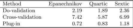
Table 1. Comparison of asymptotic variances among bandwidth selection methods: factor ΨK,• defined in Corollary 2.
Method Epanechnikov Quartic Sextic Do-validation 2.19 1.89 2.36 Cross-validation 7.42 5.87 6.99
Plug-in 0.72 0.83 1.18
factor ΨK,•for the Epanechnikov kernel, the quartic kernel and the sextic kernel. The last kernel has been used in our empirical studies. Plug-in rules achieve the same asymptotic limit as the MISE-optimal bandwidth under appropriate conditions. Thus, the value of ΨK,•for plug-in rules in Table 1 is identical to ΨK,M ISE. When comparing these constants
one has to take into account that the term S2 has to be added to get the value of the asymptotic variance. This makes the difference between Do-validation and plug-in rather small. Do-validation works under weaker conditions than required for plug-in rules. As in the discussion of Do-validation for density estimation this gives strong evidence for a good performance of Do-validation.
5. A discrete formulation in terms of occurrences and exposures
In this section we write the local linear estimator as a function of occurrences and exposures, see (1). Also we will always choose natural weightingW(s)≡ 1. Typically survival data are not provided as continuous data, in contrast to our continuous model. They are given as aggregated numbers. One reason data providers use this data format is to reduce data size. Another reason might be tradition and habit.
The mortality data that we will use are divided into discrete yearly numbers of oc-currences and exposures. This data only allow an approximation of the fully continuous filtered model as it is formulated in this paper. However, one can show that the approx-imation is sufficiently precise to provide a reasonable fit to the continuous model. We now describe a modification of the local linear estimator for discrete data. We suppose that the following aggregated values of occurrences and exposures are available: Or =
Pn i=1
RXr
Xr−1dNi(x) and Er=
Pn i=1
RXr
Xr−1Yi(x)dx forr= 1, . . . , m. Here, X1, . . . , Xm are
some time points. We allow that they are not equidistant. In particular, this may be the case if the data are transformed to another scale for statistical reasons as we will see in Section 7 below. With ∆r = Xr−Xr−1 we can define Yr = Er/∆r. This is the
aver-age number of individuals which are at risk in the interval [Xr−1, Xr) for r = 1, . . . , m
and with X0 = 0. The discrete versions of the estimators OLL(t) and ELL(t) can now
be defined as Od,LL(t) = Pmr=1(ad,2(t)−ad,1(t)(t−Xr∗))Kb(t−Xr∗)Or and Ed,LL(t) =
Pm
r=1(ad,2(t)−ad,1(t)(t−Xr∗))Kb(t−Xr∗)Er, wheread,j(t) =Pmr=1Kb(t−Xr∗)(t−Xr∗)jEr, j = 0,1,2, and Xr∗ = (Xr−1+Xr)/2, for r = 1, . . . , m. Finally the discrete version of
the local linear hazard estimator is given as the ratio αbb,d,LL(t) = EOd,LLd,LL((tt)). Withαe[b,d,LLr]
defined as the estimator after replacingOr byOr−1, the cross-validation bandwidth can
be defined as the minimizer ofPmr=1(αeb,d,LL(Xr∗))
2
Er−2Pmr=1αe [r]
b,d,LL(Xr∗)Or.
Ramlau-40 50 60 70 80 90 100 110
0.0
0.5
1.0
1.5
UK − Hazard estimate
age
DO CV 95% C.I.
100 102 104 106 108 110
0.4
0.8
1.2
1.6
UK − Hazard estimate
age
Zoom: old−age mortality
40 50 60 70 80 90 100 110
0
4000
8000
12000
Smoothed occurrences
age
100 102 104 106 108 110
0
200
600
1000
Smoothed occurrences
age
Zoom: old−age mortality
40 50 60 70 80 90 100 110
0e+00
2e+05
4e+05
Smoothed exposures
age
100 102 104 106 108 110
0
500
1500
2500
Smoothed exposures
age
[image:11.595.123.450.113.366.2]Zoom: old−age mortality
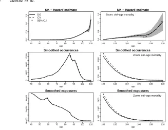
Fig. 1. Case study with mortality data. The top panels show the estimated local linear hazard with
95% confidence bands. The panels below display the two components of the hazard estimators
Od,LL(t)andEd,LL(t), defined in Section 5, for United Kingdom. The solid line is obtained using the Do-validation method and the dashed line with cross-validation.
Hansen weighting. Tutz and Pritscher (1996) suggested a discretized version but for the local constant estimator which is the simple Ramlau-Hansen estimator.
6. The local linear hazard estimator in practice
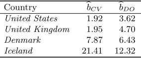
Table 2. Case study with mortality
data. Estimated bandwidth for each country using the cross-validation and the Do-validation methods.
Country bbCV bbDO
[image:12.595.247.389.168.227.2]United States 1.92 3.62 United Kingdom 1.95 4.70 Denmark 7.87 6.43 Iceland 21.41 12.32
Table 3. Old-age mortality data from Iceland. Original data given as occurrences and exposures
and the ratio between them.
Age 100 101 102 103 104 105 106 107 108 109
Occurrences 6 3 3 1 0 0 1 0 0 2
Exposure 11.50 6.83 2.50 1.33 0.50 0.50 0.17 0.00 1.00 0.33
Ratio 0.522 0.439 1.20 0.752 0.000 0.000 5.882 0 0.000 6.061
We now use the Iceland data to compare natural weights and Ramlau-Hansen weights in local linear smoothing, see the discussion at the end of Section 2. Table 3 gives the observed occurrences/exposures for individuals in Iceland at the ages from 100 to 109. The empirical estimator of the hazard at age 106 is extremely large. The reason is that one death was recorded during this period and that the exposure was only 0.17. This value comes from one 106 years old individual who died in March. The local linear estimators with natural weighting and Ramlau-Hansen weighting are shown in the left plots of Figure 2. We now modify the data and replace the value of exposure for age 106 by 0.005. This very low exposure value would have been reported if the individual would have died in early January instead of in March. The new modified data are shown in Table 4. The resulting new local linear estimators are given on the right hand side of Figure 2. We see that local linear smoothing with natural weights is rather robust. There are nearly no changes of the estimator. On the other hand local linear smoothing with Ramlau-Hansen weights shows drastic changes on the right tails. Note that these changes are caused by a minor change of the data. We argue that this instability also occurs if the number of cases at the boundary is slightly larger. We therefore recommend to use natural weighting instead of Ramlau-Hansen weighting. See also Nielsen and Tanggard (2001) and Nielsen et al. (2009) for more details about this issue.
7. Simulation studies
In this section we compare the finite sample performance of Do-validation bandwidths and cross-validation bandwidth estimates and show that Do-validation corrects some of the
Table 4. A modification in the old-age mortality data from Iceland. The original exposure at the age
of 106 has been replaced by the value 0.005 so that the ratio between occurrences and exposures increases dramatically at this age.
Age 100 101 102 103 104 105 106 107 108 109
Occurrences 6 3 3 1 0 0 1 0 0 2
Exposure 11.50 6.83 2.50 1.33 0.50 0.50 0.005 0.00 1.00 0.33
[image:12.595.123.515.260.305.2] [image:12.595.121.515.652.698.2]95 100 105 110
0.5
1.0
1.5
2.0
Exposure: 0.17
95 100 105 110
0
5
10
15
20
25
Exposure: 0.005
95 100 105 110
0.5
1.0
1.5
2.0
2.5
Exposure: 0.17
95 100 105 110
0.5
1.0
1.5
2.0
2.5
[image:13.595.190.419.127.279.2]Exposure: 0.005
Fig. 2. Exposure robustness analysis of two possible weightings for the local linear hazard estimator:
Ramlau-Hansen weighting and natural weighting. The left panels show the hazard estimates from the original old-age mortality data in Iceland (Table 3). The right panels show the hazard estimates obtained from the modified data in Table 4.
well known drawbacks of standard cross-validation such as (i) variability of the bandwidth selector, (ii) bias of the bandwidth selector, and (iii) probability of local minima when selecting the bandwidth, see for example Loader (1999) or Hurvich et al. (1998). We present two different sampling schemes to simulate data from five hazard functions in the next subsections. The first four hazard functions are: α1(t) =B(t,2,2),α2(t) =B(t,4,4),
α3(t) = 0.6[B(t,0.5,0.5) +B(t,7,7)],α4(t) = 0.6[B(t,0.5,0.5) +B(t,4,2) +B(t,2,4)]. Here
B(t, a, b) is the density att of a Beta distribution with parameters (a, b). These hazard functions have also been used in the simulations in Nielsen and Tanggard (2001). The fifth hazard function is the parametric model estimated by Spreeuw et al. (2013) using the mortality data described in the previous section. This hazard can be written as α5(t) = (1 +σ2)−1exp(a
0+a1t+a2t2)/R0texp(a0+a1s+a2s2)ds, whereθ= (a0, a1, a2, σ2)t is a four-dimensional parameter. Here we have considered the maximum likelihood estimates of the parameters calculated from the data corresponding to Iceland (see Spreeuw et al. (2013) for more details). A plot of the five hazard models is provided in the supplementary material. For each hazard datasets are simulated with and without left-truncation.
7.1. Case 1: Without left-truncation
The data are simulated in a discrete grid of time points on the time interval. For models 1 to 4 the time interval is (0,1) and the grid length δM = 1/(M + 1). For model 5 time
is age and it lies in the interval (40,110) with grid length δM = 70/(M + 1). The grid
points are denoted by{tr, r = 1, . . . , M}. Then for a sample ofn individuals, failures at
timetr, denoted asOr are generated from the binomial distribution Bi(Yr, αk(tr)δM), for r= 1, . . . , M. Here Yr denotes the size of the risk set at the beginning of the rth interval
Samples are generated with sample sizesn= 100,1000 and 10000 for models 1 to 4 and
n= 50000,75000 and 100000 for model 5 (this is comparable to the sample sizen=64630 of the mortality dataset). The number of Monte Carlo replications isR= 1000. The grid size has been chosen equal toM = 500. We have experimented with other choices of M and found that this choice is enough to provide stable results. The local linear hazard estimator has been calculated using the sextic kernel: K(x) = 3003/2048(1−x2)6I(−1< x <1). For each model and sample size we compare the performance of the two bandwidth estimates presented in Section 3: the Do-validated bandwidthbbDO and the cross-validated bandwidth
bbCV. As benchmarks we calculate two infeasible bandwidths: the ISE-optimal bandwidth
bbISE and the MISE-optimal bandwidthbbM ISE. The MISE is approximated by the average
of the ISE errors along the R simulated samples. The MISE-optimal bandwidth bbM ISE
is approximated by the bandwidth minimizing this average value. We consider a grid of 100 equispaced bandwidth values around the ISE-optimal bandwidth to compute these four bandwidths. The performance of the bandwidth estimates is analysed with respect to three performance measures, which we denote by m1, m2 and m3, see Table 5. For any bb=bbDO,bbCV,bbISE,bbM ISE, the measurem1(bb) denotes the (Monte Carlo estimate of the) MISE of the local linear hazard estimatorαbbb,K. The bandwidths are compared to the ISE-optimal bandwidth by the measurem2 which is defined as the average of the differences bb−bbISE. Thusm2is a Monte Carlo estimate of the bias ofbbwith respect to the ISE-optimal bandwidth. Finally we have calculatedm3which is the standard deviation of the differences bb−bbISE.
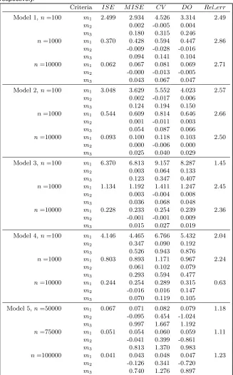
Table 5 shows the simulation results in the above scenarios. Another measure has been added evaluating the relative loss of using Do-validation respectively cross-validation to using the infeasible ISE-optimal bandwidth. The measure is defined as: Rel err =
{m1(bbCV)−m1(bbISE)}/{m1(bbDO)−m1(bbISE)}. Note that Rel err indicates when
Do-validation outperforms cross-Do-validation considering the criterionm1. This is the case when this value is above 1. We can see from Table 5, that Do-validation is better than cross-validation for all models and sample sizes. We also see that the improvement from using Do-validation is substantial with a relative error that is often above 2. There is only one out of twelve cases where the result of cross-validation is better than for Do-validation. An inspection of them2-values shows that cross-validation has a tendency to undersmooth while Do-validation is slightly oversmoothing. The absolute value of the bias terms were smaller for Do-validation in the first three models and they were smaller for cross-validation in the remaining two. Considering the criterionm3, we can see thatbbDO outperformsbbCV
in almost all cases.
7.2. Case 2: With left-truncation
When adding left truncationLionly individuals withLi≤Ziare entering the dataset in the
simulations andY(n)(t) is defined asPn
i=1I(Li ≤t≤Zi), withLi andZi as in Section 2. The left truncation times are simply generated by independent variables from the uniform distribution. Besides these changes, values of exposures and occurrences are generated in the same way as in the previous section. The performance of the bandwidth estimates are again analysed using the same criteriam1,m2and m3 described above. Also in this more complex model with left truncation Do-validation shows excellent performance properties. For all specifications of the model, Do-validation clearly outperforms cross-validation with
Table 5. Simulation results for datasets without left-truncation. Measure m1 in
columns 3–6 is the empirical MISE for each bandwidth estimate (multiplied by 100 for models 1 to 4 and by 1000 for model 5). The last column shows the relative error
Rel errthat compares Do-validation with standard cross-validation. Measuresm2
and m3 are the average and the standard deviation of the differencesbb−bbISE,
respectively.
Criteria I SE M I SE CV DO Rel err
Model 1,n=100 m1 2.499 2.934 4.526 3.314 2.49 m2 0.002 -0.005 0.004
m3 0.180 0.315 0.246
n=1000 m1 0.370 0.428 0.594 0.447 2.86 m2 -0.009 -0.028 -0.016
m3 0.094 0.141 0.104
n=10000 m1 0.062 0.067 0.081 0.069 2.71 m2 -0.000 -0.013 -0.005
m3 0.043 0.067 0.047
Model 2,n=100 m1 3.048 3.629 5.552 4.023 2.57 m2 0.002 -0.017 0.006
m3 0.124 0.194 0.150
n=1000 m1 0.544 0.609 0.814 0.646 2.66 m2 0.001 -0.011 0.003
m3 0.054 0.087 0.066
n=10000 m1 0.093 0.100 0.118 0.103 2.50 m2 0.000 -0.006 0.000
m3 0.025 0.040 0.029
Model 3,n=100 m1 6.370 6.813 9.157 8.287 1.45 m2 0.003 0.064 0.133
m3 0.123 0.347 0.407
n=1000 m1 1.134 1.192 1.411 1.247 2.45 m2 0.003 -0.004 0.008
m3 0.036 0.068 0.048
n=10000 m1 0.228 0.233 0.254 0.239 2.36 m2 -0.001 -0.001 0.009
m3 0.015 0.027 0.019
Model 4,n=100 m1 4.146 4.465 6.766 5.432 2.04 m2 0.347 0.090 0.192
m3 0.526 0.943 0.876
n=1000 m1 0.803 0.893 1.171 0.967 2.24 m2 0.061 0.102 0.079
m3 0.293 0.594 0.477
n=10000 m1 0.244 0.254 0.289 0.315 0.63 m2 -0.016 0.016 0.147
m3 0.070 0.119 0.105
Model 5,n=50000 m1 0.067 0.071 0.082 0.079 1.18 m2 -0.095 0.454 -1.024
m3 0.997 1.667 1.192
n=75000 m1 0.051 0.054 0.060 0.059 1.11 m2 -0.041 0.399 -0.861
m3 0.813 1.370 0.983
n=100000 m1 0.041 0.043 0.048 0.047 1.23 m2 -0.126 0.341 -0.720
[image:15.595.148.475.186.712.2]We have checked cross-validation and Do-validation for the number of local minima in their criterion functions. This has been done by evaluating the criterion on a fine grid of bandwidth values. We have calculated the percentage of times where the score in (4) for the kernel K (cross-validation) or for the one-sided kernels KL and KR (Do-validation) have
more than one minima on the considered grid of bandwidths. The small number of cases where the Do-validation criterion runs into having several local minima is an indicator for the stability of Do-validation compared to cross-validation. Our results for both models, with and without truncation, show that cross-validation presents multiple local minima in a percentage of cases ranging from 2.0 to 21.2, with a median of 9.8, while Do-validation provides percentages ranging from 0.0 to 2.4, with a median of 0.0. A table with the full summary is provided in Table 2 in the supplementary material of this paper.
8. Hazard estimation for transformed data
In this section we propose a two-step procedure for hazard estimation. First a parametric hazard functionλθ
i(t) =αθ(t)Yi(t) with θ∈Θ is fitted to the data. This parametric fit is
used to transform the data in such a way that the underlying hazard would become constant in case the parametric fit indeed would have been the correct underlying model. The para-metric fit is in other words used as a kind of prior knowledge to simplify the nonparapara-metric estimation problem. If the prior knowledge is of high quality and the parametric model has good approximation properties, then the resulting nonparametric problem is simplified in the second step. In the second step a local linear hazard estimator is applied to the trans-formed data. The resulting semiparametric estimator is an alternative to the original fully nonparametric estimator and it is expected to do a better job when the used parametric model is accurate enough.
If the parametric specificationαθwere true then after the time transformationx= Λθ(t)
with Λθ(t) =
Rt
0αθ(s)dsthe functional form of the hazard on the transformed scale would be simply equal to the standard exponential. That is, the hazard would be equal to one on the transformed scale.
For a givenθ∈Θ we putNeθ
i =Ni◦Λ−1θ andYeiθ=Yi◦Λ−1θ . This transformed process
follows Aalen’s multiplicative hazard model with transformed stochastic hazard eλθi(x) = gθ(x)Yi Λ−1θ (x)
,wheregθ(x) =α Λ−1θ (x)
/αθ Λ−1θ (x)
,αis the true hazard, andαθis
the assumed parametric value. We now carry out our nonparametric local linear smoothing technique on the transformed processesNeθ
i andYeiθand obtain an estimategbθofgθ on the
transformed time axis. These plots can also be used as a check of the parametric model, see Spreeuw et al. (2013). This is illustrated below by a data example. After back transforming to the original scale we get the semiparametric hazard: αbθ(t) =bgθ(Λθ(t))αθ(t).In practice θ is estimated. One could for example use the maximum likelihood estimator θbof θ, see Borgan (1984).
40 50 60 70 80 90 100 110
0.0
0.5
1.0
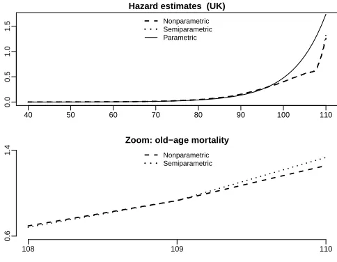
1.5
Hazard estimates (UK)
Nonparametric Semiparametric Parametric
Zoom: old−age mortality
108 109 110
0.6
1.4 Nonparametric
[image:17.595.185.427.130.318.2]Semiparametric
Fig. 3. Hazard estimators with Do-validated bandwidths in the case study for United Kingdom: the
parametric estimator, the semiparametric estimator withbbDO= 5.87; and the nonparametric
estima-tor withbbDO= 4.70. The bottom panel shows the maximum difference between the semiparametric and the nonparametric estimators at the highest age is about 8% .
(2013) implies that the underlying continuous data come from a counting process with inten-sity function λθ
i(t) = (1 +σ2)−1exp(a0+a1t+a2t2)( Rt
0exp(a0+a1s+a2s
2)ds)−1Y
i(t) = αθ(t)Yi(t), whereθ= (a0, a1, a2, σ2)tis a four-dimensional parameter.
The final semiparametric approach used in our application was first to calculate the parametric maximum likelihood estimators ofθfollowing Borgan (1984) and then to trans-form the time axis with the function Λbθ, where Λθis the integrated hazard function of the
underlying hazardαθ. Finally, a local linear hazard was estimated to the transformed data
and the resulting nonparametric estimator was backtransformed to the original axes. We have compared the resulting hazard estimators from the semiparametric approach with the fully nonparametric local linear estimator considered in Section 2 and the just discussed parametric specification. In general the three estimates are quite close except for the old-age mortality where relative differences up to 8% are found. Semiparametric test theory goes along the lines of many other semiparametric test procedures from survival analysis, see among many others Gandy and Jensen (2005), to evaluate the quality of the parametric transformation approach.
Acknowledgements
de Inform´atica y Redes de Comunicaciones (CSIRC), Universidad de Granada, for provid-ing the computprovid-ing resources. Support by Deutsche Forschungsgemeinschaft through the Research Training Group RTG 1953 is gratefully acknowledged. Research of the second author was prepared within the framework of a subsidy granted to the HSE by the Gov-ernment of the Russian Federation for the implementation of the Global Competitiveness Program. Finally we thank the Associate Editor and two anonymous reviewers for their constructive comments.
A. Details on the asymptotics and proof of Theorem 1
In this section we describe the assumptions made for the asymptotic theory, introduce additional notation, and provide the proof of the main result.
Assumptions
(A1) (i) For the expected exposure function γ(t) =n−1E[Y(n)]it holds that γ∈C
2([0, T]), that it is strictly positive for t ∈ [0, T], and that sups,t∈[0,T],|t−s|≤CKb|[Y
(n)(t)−
Y(n)(s)]/n−[γ(t)−γ(s)]| =o
P((nblogn)−1/2) and sups∈[0,T]
Y(n)(s)/n−γ(s)=
oP((logn)−1),where the constant CK is defined in (A2).
(ii) The weight W is a predictable process. There exists a function γ∗ ∈ C
2([0, T]), that is strictly positive fort∈[0, T], and that fulfills with the same constantCK as in
(i) that sups∈[0,T]|W(s)−γ∗(s)|=o
P((logn)−1) and sups,t∈[0,T],|t−s|≤CKb[W(t)−
W(s)]/−[γ∗(t)−γ∗(s)]|=oP((nblogn)−1/2).
(A2) The kernels K and Lj (j = 1, ..., J) are compactly supported (i.e., the support is
contained in [−CK, CK] for some constants CK > 0). The kernels are continuous
on IR\{0} and have one-sided derivatives that are H¨older continuous on IR− ={x:
x < 0} and IR+ = {x : x > 0}, that is there exist constants c and δ such that
|g(x)−g(y)| ≤c|x−y|δ forx, y <0orx, y >0withgequal toK′ orL′
j (j= 1, ..., J).
The left and right-sided derivatives differ at most on a finite set. The kernel K is symmetric.
(A3) It holds that α ∈ C2([0, T]), w ∈ C1([0, T]). The second derivative of α is H¨older continuous with exponentδ >0.
Assumptions (A1)–(A3) are rather weak. Assume for instance thatYi(t) = I(Li≤t < Zi)
for some i.i.d. tuples (Li, Zi) with joint continuously differentiable density. Then
Assump-tion (A1)(i) can be easily verified withγ(t) =P(Li ≤t < Zi). For the weightW(s)≡1
Assumption (A1)(ii) holds trivially. For Ramlau-Hansen weighting W(s) = {n/Y(n)(s)}
I(Y(n) >0) it follows from Assumption (1)(i). Assumption (A2) is a weak standard con-dition on kernels. Assumption (A3) differs from standard smoothness concon-ditions only by the mild additional assumption that the second derivative of the hazard function fulfils a H¨older condition.
We now state and prove some lemmas that we will use in the proof of Theorem 1. For simplicity we assume in the proof that the weight functionW is deterministic. If this is not the caseW can be treated in the same way as we will do it in the proof for the analysis of
Y(n)(t)/n. As in the expression above (2) forL=L
jwithj = 1, . . . , J andL=Kthe local
linear estimatorsαbb,Lare defined asαbb,L(t) =Pni=1 RT
defined as in (2). We also defineα∗
b,L(t) =
RT
0 L¯t,b(t−s)W(s)α(s)Y
(n)(s)ds.Thus we have
thatαbb,L(t)−α∗b,L(t) =
Pn i=1
RT
0 L¯t,b(t−s)W(s)dMi(s) = RT
0 L¯t,b(t−s)W(s)dM(s). To prove the main result in the paper we first state a uniform asymptotic expansion for the Integrated Squared Error (ISE). Similar expansions are well known for other kernel smoothing estimators but they require some additional work in the hazard case. As outlined before the statement of Theorem 1, the interval I∗
n = [a∗1n−1/5, a∗2n−1/5] is defined with constantsa∗
2> a∗1>0 that fulfill a∗1< C0,L< a2∗ forL=K andL=Lj withj= 1, ..., J.
Lemma 3. Under A1–A3, we get for the ISE, ∆L(b), with kernels L=K andL=Lj
(j= 1, . . . , J) that, uniformly for b∈I∗
n,∆L(b) =ML(b) +oP n−4/5
.
Proof. For brevity we write αb = αbb,L and α∗ = α∗b,L. We have that ∆L(b) =
n−1RT
0 [αb(t)−α ∗(t)]2
Y(n)(t)w(t)dt+ 2n−1RT
0 [αb(t)−α
∗(t)] [α∗(t)−α(t)]Y(n)(t)w(t)dt+
n−1RT 0 [α
∗(t)−α(t)]2
Y(n)(t)w(t)dt. Below we will apply a martingale central limit theo-rem. We cannot directly apply this theorem to ∆L(b) because the integrand in the definition
ofαb(t) is not predictable. More precisely, the integrand ofαb(t) contains values ofY(n)(s) withs > tin the termsaL
l,b(t) forl= 0,1,2. For this reason we use an approximationdb∗(t)
ofαb(t)−α∗(t) whereY(n)(s) is replaced byY(n)(t) +n{γ(s)−γ(t)}. We will show that
(logn)1/2n1/2b1/2bα(t)−α∗(t)−db∗(t)=oP(1), (9)
uniformly for 0 ≤ t ≤ T and b ∈ I∗
n, where db∗(t) =
Pn i=1
RT
0 L¯ +
t,b(t−s)W(s) dMi(s) =
RT
0 L¯ +
t,b(t−s)W(s)dM(s), ¯L
+
t,b(u) =
a+2,b(t)−a+1,b(t)u
a+0,b(t)a+2,b(t)−{a1+,b(t)}2Lb(u), Lb(u) = b
−1L(b−1u) and
a+l,b(t) = R0TLb(t−s)(t−s)lW(s)
Y(n)(t) +n{γ(s)−γ(t)}ds for j = 1, . . . , J and l = 0,1,2. Note that the integrand in the definition ofdb∗(t) is predictable. Expansion (9) follows directly from Assumption (A1). We now apply (9), Assumption (A1) and supt∈[0,T]
bd∗(t)
=
OP((logn)1/2(nb)−1/2) and supt∈[0,T]|α∗(t)−α(t)|=OP((nb)−1/2). This gives that
∆L(b) =
Z T
0 b
d∗(t)2γ(t)w(t)dt+ 2 Z T
0 b
d∗(t) [α∗(t)−α(t)]γ(t)w(t)dt
+ Z T
0
[α∗(t)−α(t)]2γ(t)w(t)dt+oP(n−4/5)
= SL,1(b) +SL,2(b) +TL,1(b) +TL,2(b) +oP(n−4/5),
uniformly forb∈I∗
n, whereSL,1(b) = RT
0 H¯L,b(u, v)dM(u)dM(v)− RT
0 H¯L,b(u, u)α(u)γ(u)
du,SL,2(b) = 2R0TδL,b(u)dM(u),TL,1(b) =R0TH¯L,b(u, u)α(u)γ(u)du,TL,2(b) =R0T[α∗(u)
−α(u)]2γ(u)w(u)du, ¯H
L,b(u, v) =R0TL¯+t,b(t−u) ¯L+t,b(t−v)W(u)W(v)γ(t)w(t)dt,δL,b(u) =
RT
0 L¯ +
t,b(t−u)W(u) [α∗(t)−α(t)]γ(t)w(t)dt.
We now argue that uniformly for b∈ I∗
n it holds thatSL,1(b) and SL,2(b) are of order
oP n−4/5, and thatTL,1(b) = (nb)−1R( ¯L∗)R0Tα(t)w(t)dt+oP n−4/5,TL,2(b) =b4µ22( ¯L∗) RT
0
α′′(t)
2 2
γ(t)w(t)dt+oP n−4/5. We will show the first statement. The second claim
smoothing theory arguments using that uniformly forb∈I∗
n,CLb≤t≤T−CLb it holds
thatR( ¯L+t) =R( ¯L∗) +o(1) andµ2( ¯L+t) =µ2( ¯L∗) +o(1).
For the proof of SL,1(b) = oP n−4/5, uniformly for b ∈ In∗, we consider the process x→ZT,n(x), with
Zt,n(x) =n4/5
Z t
0 Z t
0 ¯
HL,xn−1/5(u, v)dM(u)dM(v)−n4/5
Z t
0 ¯
HL,xn−1/5(u, u)α(u)γ(u)du,
withx∈[a∗
1, a∗2]. Note thatZT,n(x) =n4/5SL,1(xn−1/5). Thus for forSL,1(b) =oP n−4/5
we have to show that
sup
x∈[a∗
1,a∗2]
|ZT,n(x)| = oP(1). (10)
We first show pointwise convergence
ZT,n(x) = oP(1) (11)
for x ∈ [a∗
1, a∗2]. Now, for x ∈ [a∗1, a∗2] fixed, we get that t → Zt,n(x) is a martingale.
This follows from the representation: Zt,n(x) =
Rt
0Rn(w, x) dM(w) with Rn(w, x) =
n4/5Rw
0 2 ¯HL,b(u, w)I[u 6= w]γ(u) dM(u)−H¯L,b(w, w) and the fact that Rn(t, x) is pre-dictable with respect to the filtration (Ft)t≥0. For the proof of (11) we will apply a mar-tingale central limit theorem. We state a central limit theorem instead of a simpler law of large numbers because we will make use of the central limit theorem again below. Suppose that for someσ2≥0 and a martingaleV
t,n=
Rt
0Wn(w)dM(w) with an (Ft)t≥0predictable processWn(t) we have that:
Z T
0
Wn2(t)Y(n)(t)α(t)dt=σ2+oP(1), (12)
Z T
0
Wn2(t)I[Wn2(t)> ε]Y(n)(t)α(t)dt=oP(1) for allε >0. (13)
Then it holds that
VT,n=
Z T
0
Wn(w)dM(w)→N(0, σ2), in distribution. (14)
For a discussion of this central limit theorem, see e.g. Ramlau-Hansen (1983). In the proof of (11) we apply this result withσ2= 0 andW
n(t) =Rn(t, x). Then (12) implies (13) and
for (11) we have to show thatR0TR2
n(t, x)Y(n)(t)α(t)dt=oP(1) for allx∈[a∗1, a∗2]. Because of (A1) this claim follows fromnR0TR2
n(t, x)dt=oP(1). This immediately follows fromn
E[R0TRn(t, x)2dt] =o(1). This concludes the proof of (11).
For the proof of (10) we have to show that the processx→ZT,n(x) is tight. For this
purpose we apply the tightness criterion (12.51) in Billingsley (1968). For (10) it suffices to show that E[{ZT,n(x1)−ZT,n(x2)}2] ≤ C(x1−x2)2 for some constant C and for all
For the asymptotic discussion of the cross-validation selectorbbL
CV note that minimizing
b
QL(b) is equivalent to the minimization of
b
∆L(b) =QbL(b) +n−1
Z
α(t)2w(t)Y(n)(t)dt+ 2n−1
Z
α(t)w(t)dM(t).
The two last terms in ∆bL(b) do not depend on the bandwidth b. Thus, the minimizer of
b
∆L(b) is equal to the CV-bandwidthbbLCV. Note also that it holds that
b
QL(b) =n−1
(Z T
0
[αbb,L(s)]2Y(n)(s)w(s)ds−2
Z T
0 b
α−b,L(s)w(s)dN(s) )
,
whereαb−b,L(t) =R0TL¯t,b(t−s)W(s)I[s6=t]dN(s).
The next lemma states consistency of cross-validation.
Lemma 4. Under A1–A3, we get for L=K andL=Lj (j = 1, ..., J) that D1,L(b) =
∆L(b)−∆bL(b) = oP n−4/5, uniformly for b ∈ In∗. In particular, we have thatbbLCV = bL
M ISE+oP n−1/5.
Proof. For brevity we write, as in the proof of Lemma 3, αb =αbb,L, αb− =αb−b,L and
α∗=α∗
b,L. By simple calculations one gets that
nD1,L(b) = 2
Z T
0
[αb−(s)−α(s)]w(s)dM(s) + 2 Z T
0
[αb−(s)− b
α(s)]w(s)Y(n)(s)α(s)ds
= 2n−1
Z T
0
[αb−(s)−α(s)]w(s)dM(s)
= 2 Z T
0
[αb−(s)−α∗(s)]w(s)dM(s) + 2 Z T
0
[α∗(s)−α(s)]w(s)dM(s)
= nU1,L(b) +nU2,L(b).
We will show that
U1,L(b) = U1∗,L(b) +oP(n−4/5) (15)
uniformly forb∈I∗
n, whereU1∗,L(b) = 2n−1
RT
0 db
−(s)w(s)dM(s) anddb−(t) =Pn i=1
RT
0 L¯ +
t,b(t− s)I(s6=t)W(s)dMi(s) with ¯L+t,b defined as in the proof of Lemma 3.
With similar arguments as in the proof of Lemma 3 one can show that both terms,
U∗
1,L(b) andU2,L(b) are of orderoP(n−4/5). This givesD1,L(b) =oP(n−4/5). Using similar
arguments as in the proof of Lemma 3 one can show that the convergence is uniform. This implies the statement of Lemma 4. It remains to show (15).
For the proof of (15) we apply Lemma A1 in Mammen and Nielsen (2007). For this pur-pose we write: U1,L(b)−U1∗,L(b) =
Pn i=1
RT
0 hi(s)dMi(s) withhi(s) =n −1P
j6=i
RT
0 ( ¯Ls,b− ¯
L+s,b)(s−t)dMj(t). According to Lemma A1 in Mammen and Nielsen (2007) it holds that
E(U1,L(b)−U1∗,L(b))2≤ n
X
i=1
ρ2i +n n
X
i=1
whereρ2
i =E[
RT
0 h2i(s)Yi(s)α(s)ds] andδ2i ≡E[
RT
0
n−1RT
0 ( ¯Ls,b−L¯ +
s,b)(s−t)dMj(t)
2
Yi(s)α(s)ds] withj6=i. We now use that because of Assumption (A1) for a constantC >0
we have that|( ¯Ls,b−L¯+s,b)(s−t)| ≤Cn−1n−2/5(logn)−1/2n1/5=Cn−6/5(logn)−1/2. This
implies the following bound forδ2
i with some constantsC1, C2, ... >0:
δi2 ≤ C1n−2n−12/5(logn)−1
×E
"Z T
0 Z T
0 Z T
0
I(|t−s| ≤C2n−1/5)I(|u−s| ≤C2n−1/5)dMj(t)dMj(u)ds
#
≤ C3n−22/5(logn)−1
Z T
0 Z T
0
I(|t−s| ≤C2n−1/5)dt ds≤C4n−23/5(logn)−1.
By using similar bounds one gets that ρ2
i ≤ C5n−18/5(logn)−1. Thus, we have that
E(U1,L(b)−U1∗,L(b))2 ≤ C6n−13/5(logn)−1.We now argue that for two bandwidths b1,
b2 with |b1 −b2| ≤ n−3/5(logn)−1/2 it holds that |[U1,L(b1)−U1∗,L(b1)]−[U1,L(b2)−
U∗
1,L(b2)]| ≤C7n−2/5(logn)−1/2|b1−b2|n1/5≤C7n−4/5(logn)−1, where again Assumption (A1) has been used. The last inequality implies that it suffices to show supb∈I∗∗
n |U1,L(b)−
U∗
1,L(b)| = oP(n−4/5), where In∗∗ is a finite subset of In∗ with less than C8n2/5(logn) ele-ments. Here,I∗∗
n can be chosen as a grid of points that is contained inIn∗and where
neigh-bored points have a distance less than or equal ton−3/5(logn)−1. Now forδ >0 it holds that Psupb∈In∗∗|U1,L(b)−U1∗,L(b)|> δn−4/5
≤Pb∈I∗∗n P |U1,L(b)−U
∗
1,L(b)|> δn−4/5
≤Pb∈I∗∗n E
U1,L(b)−U1∗,L(b)
2
δ−2n8/5 ≤C
8n2/5 (logn)C6n−13/5(logn)−1δ−2n8/5 =C9
δ−2n−3/5. Because this upper bound converges to 0 we get that (15) holds. This concludes the proof of the lemma.
The next lemmas enable us to develop linear expansions of bbL
ISE. For functions G
depending on the bandwidthbwe denote byG′andG′′the first or second derivative of this function w.r.t.b, respectively.
Lemma 5. Under A1–A3, we get for L = K andL =Lj (j = 1, ..., J) that ∆′′L(b) =
M′′
L(b) +oP n−2/5 andD′′1,L(b) =oP n−2/5uniformly forb∈In∗.
Proof. This lemma can be shown with similar arguments as used in the proof of Lemma
4. Note first that the derivative of a kernelRb(u) =b−1R(b−1u) w.r.t. to the bandwidth bis equal to b−2R∗(b−1u) =b−1R∗
b(u) with R∗(u) =−R(u)−uR′(u) and that the second
derivative is equal tob−2R∗∗
b (u) withR∗∗(u) = 2R(u) + 4uR′(u) +u2R′′(u). Thus the first
and the second derivative behave like the product of a kernel and the factor b−1 or b−2, respectively. By looking at the derivatives ofa∗
l,b(t) anda∗l,b(t) withl = 0,1,2 one can see
that the same holds true for the kernels ¯Lt,band ¯L+t,b. Using these facts one can easily treat D′′
1,L(b) as in the proof of Lemma 4. One writes D′′1,L(b) as the sum of two expressions
and one shows that the integrand in the first expression can be replaced by a predictable integrand, with an error that is now of the order oP(n−2/5), uniformly over all b. The
order of the error term is now by a factorn2/5larger because of the just outlined argument. Afterwards one argues again as in the proof of Lemma 3 that the modified first term and the second term are of orderoP(n−2/5), uniformly over allb, where the error rate is again
For the expansion of ∆′′
L(b) one replacesαb(t)−α∗(t) and its derivatives bydb∗(t) and its
derivatives. Using brute force bounds as in the proof of Lemma 3 one gets that ∆′′
L(b) = S′′
L,1(b) +SL,′′2(b) +TL,′′1(b) +TL,′′2(b) +oP(n−2/5), whereSL,1(b),SL,2(b),TL,1(b) andTL,2(b) are defined as in Lemma 3.
One now shows thatS′′
L,1(b) =oP n−2/5
,S′′
L,2(b) =oP n−2/5
,T′′
L,1(b) = 2n−1b−3R( ¯L∗) RT
0 α(t)w(t)dt+oP n
−2/5, T′′
L,2(b) = 3b2µ22( ¯L∗) RT
0 α
′′(t)2γ(t)w(t)dt+o
P n−4/5
. The proof of the first two claims is similar to the proof of (10). Furthermore, the last two state-ments follow by standard kernel smoothing theory. Note thatM′′
L(b) = 3b2µ22( ¯L∗) RT
0 α ′′(t)2
γ(t)w(t)dt+ 2n−1b−3R( ¯L∗)RT
0 α(t)w(t)dt. This concludes the proof of Lemma 5.
We now state expansions of ∆′
L(bLM ISE) andDL,′ 1(bLM ISE).
Lemma 6. Under A1-A3, we get for L =K and L =Lj (j = 1, ..., J) that with b =
bL M ISE
∆′
L(b) = −n−2b−2
Z
HL(b−1(u−v))w(u)γ(u)−1 dM(u)dM(v)
+2n−1bµ2( ¯L∗) Z
α′′(u)w(u)dM(u) +oP
n−7/10,
D′L,1(b) = −n−2b−2 Z
GL(b−1(u−v))w(u)γ(u)−1 dM(u)dM(v)
+2n−1bµ2( ¯L∗) Z
α′′(u)w(u)dM(u) +oP
n−7/10,
whereL¯∗
b(u) =b−1L∗(b−1u),L¯∗∗b (u) =b−1L∗∗(b−1u),GL(w) =I[w6= 0]( ¯L∗∗(w)−L¯∗∗(−w))
andHL(w) =I[w6= 0]RL¯∗(u)( ¯L∗∗(w+u)−L¯∗∗(−w+u))duwithL¯∗(u) = µµ22((LL)−()−µµ11((LL)))u2L(u)
andL¯∗∗(u) =−µ2(L)−µ1(L)u
µ2(L)−(µ1(L))2(L(u) +uL
′(u)) + µ1(L)u
µ2(L)−(µ1(L))2L(u). In particular, it holds
that∆′
L(b) =OP n−7/10 andD′L,1(b) =OP n−7/10.
Proof. We treat ∆′
L(b) andD′L,1(b) in two steps. In a first step one can use the results in Mammen and Nielsen (2007) to show that replacing the kernels ¯Lt,b(u) and∂bL¯t,b(u) by
the kernels ¯L+t,b(u) or ∂bL¯+t,b(u), respectively, leads to an error of order oP n−7/10
. The arguments are similar to the proof of Lemma 4. But the argumentation is now simpler because we expand the functions ∆′
L(b) and DL,′ 1(b) for one value of b and not uniformly for a set of values ofb. In a next step the kernels ¯Lt,b(u) and∂bL¯t,b(u) are replaced by the
kernels (W(t)γ(t))−1L¯∗
b(u) or (W(t)γ(t)b)−1 L¯∗∗b (u), respectively. This gives an additional
error term of order oP n−7/10. This can be proved by the calculation of the first two
moments of the approximations of ∆′L(b) and D′L,1(b). Note that the calculation of the fist two moments is simplified by the first step because some non-predictable integrands have been replaced by predictable functions. A check of the last approximation shows the statement of the lemma.
Lemma 7. Under A1-A3, we get for L = K and L = Lj (j = 1, ..., J) that with
b = bL
M ISE the following two expansions hold: bbLISE = b+C
−1
1,Ln−8/5b−2
R
HL(b−1(u− v))w(u)γ(u)−1 dM(u)dM(v)−2n−3/5C−1
1,Lbµ2( ¯L∗) R
α′′(u)w(u)dM(u) +o
P n−3/10
and bbL
CV =b+C
−1
1,Ln−8/5b−2
R
[HL−GL](b−1(u−v))wγ((uu)) dM(u)dM(v) +oP n−3/10
, where
C1,L= 5R( ¯L∗)2/5µ62/5( ¯L∗) nRT
0 α(t)w(t)dt
o2/5nRT 0 α