Perfect periodic scheduling for binary tree routing in wireless networks

City, University of London Institutional Repository

Citation:

This is the accepted version of the paper.

This version of the publication may differ from the final published

version.

Permanent repository link:

Link to published version:

Copyright and reuse: City Research Online aims to make research

outputs of City, University of London available to a wider audience.

Copyright and Moral Rights remain with the author(s) and/or copyright

holders. URLs from City Research Online may be freely distributed and

linked to.

City Research Online: http://openaccess.city.ac.uk/ [email protected]

Perfect periodic scheduling for binary tree routing in

Wireless Networks

Eun-Seok Kima, Celia A. Glass†b

a_{Department of International Management and Innovation, Middlesex University}

Business School, London NW4 4BT, United Kingdom.

b_{Cass Business School, City University London, 106 Bunhill Row, London EC1Y 8TZ,}

United Kingdom.

Abstract

In this article we tackle the problem of co-ordinating transmission of data across a Wireless Mesh Network. The single task nature of mesh nodes im-poses simultaneous activation of adjacent nodes during transmission. This makes the co-ordinated scheduling of local mesh node traffic with forwarded traffic across the access network to the Internet via the Gateway notoriously difficult. Moreover, with packet data the nature of the co-ordinated trans-mission schedule has a big impact upon both the data throughput and energy consumption. Perfect Periodic Scheduling, in which each demand is itself ser-viced periodically, provides a robust solution. In this paper we explore the properties of Perfect Periodic Schedules with modulo arithmetic using the Chinese Remainder Theorem. We provide a polynomial time, optimisation algorithm, when the access network routing tree has a chain or binary tree structure. Results demonstrate that energy savings and high throughput can be achieved simultaneously. The methodology is generalisable.

Keywords:

Scheduling, OR in Telecommunications, Mobile and Ad hoc NETworks (MANETs), Combinatorial Optimization, Chinese Remainder Theorem

1. Introduction

The emerging technology of Wireless Mesh Networks (WMN) [1] provides a promising paradigm for the flexible and low-cost provision of global

net communication. Mesh routers facilitate multi-hop wireless transmission to relay data over extended distances without need for the cost, delay and disruption of installing cabled access points. Packet scheduling facilitates improved throughput, fairness between clients, reduced delays and energy conservation [2]. However, specialized scheduling methodology is required to exploit these features.

Mesh routers are typically mounted on the sides of buildings and oper-ate in two ways: firstly they service the clients who connect directly to a mesh router to gain broadband access; secondly they act as a relay to other mesh routers in forwarding content to a particular mesh router that acts as the gateway to wired infrastructure. Within each local star network the mesh router can communicate with at most one client at a time. The packet nature of transmission imposes a discrete, unit time, nature on transmis-sion schedules. Moreover, schedules which are periodic for each client are highly desirable because they provide clients with predefined transmission times between which they can conserve resources and avoid contention. The regularity of transmission reduces jitter and thus improves Quality of Ser-vice. In addition, the issue of fairness between clients can be enforced by imposing Perfect Periodic Schedule (PPS), in which clients each have peri-odic sub-schedules of appropriate relative periperi-odicity. Across a mesh network mesh routers may therefore impose local scheduling on their own clients but then need to interweave global scheduling on forwarding traffic to another mesh router. Since mesh routers are unable to multi-task, the problem of coordinating transmission across the entire routing network in the WMN is considerable. Improvement in throughput is captured by the Minimum Frame Length Schedule Problem (MFLSP) which seeks to find a schedule of minimum total duration which may then be repeated. In this article we there-fore focus on MFLSP using centrally co-ordinated periodicities to schedule packets across the network.

Several studies have been undertaken on problems of local access. Local traffic is serviced by a mesh router, and forms a local star network, each in a periodic fashion within a perfect periodic (sub)schedule. Bar-Noy et al.

a feasible perfect periodic schedule to satisfy the particular combination of requested periodicities, heuristics are used to allocated close values, according to specific criteria. Bar-Noy et al. [5] consider two objective measures of maximum and weighted average ratios between the allocated and requested periodicities. They present a few efficient heuristic algorithms to develop a perfect periodic schedule using a methodology, called tree scheduling, since it is based on hierarchical round-robin where the hierarchy is a form of tree. Bar-Noy et al. [6] develop tree based approximation algorithms for perfect periodic schedule with the objective of minimizing weighted average ratios between the allocated periodicity and requested periodicity. Brakerski et al.

[7] study the question of dispatching in a perfect periodic schedule, namely how to find the next item to schedule, given the past schedule. There are few other papers which consider PPS for telecommunications, namely [8, 9, 10, 7], but none applied to WMNs.

Some studies have been undertaken on problems of data transmission across a mesh network to carry the data from individual mesh nodes to the Internet Gateway. Different interference models have been proposed in the wireless scheduling literature. Notably, the graph interference model [11, 12, 13, 14, 15, 16, 17], where nodes interfere with other nodes in a predefined neighborhood within the network a conflict graph. If the inter-ference is restricted to the 1-hop neighborhood, then the scheduling problem reduces to the Chromatic Number Problem. More recently the physical in-terference model has been proposed [18, 19, 20, 21, 22, 23, 24, 25, 26, 2] where signal power attenuation is taken explicitly into account via the Sig-nal to Interference plus Noise Ratio (SINR) constraint that represents the actual physical interference in the wireless network. In the WMN context, interference related to broadcast noise is less of a feature. The main char-acteristic of the technology is blocking of transmission on adjacent links due to the single-task nature of mesh nodes. The problem thus resembles 1-hop edge colouring. However, the strongest feature in our context is the periodic nature of transmission through a link.

co-ordinating local schedules is to control their relative start times. How-ever, this is rarely sufficient even with sparse local schedules. Allen et al.

[27] develop an optimization scheduling algorithm which in addition equi-tably reduces the service time to local clients. Their algorithm works well for 25-node routing networks. However, by the nature of the problem, a large reduction in throughput was required to achieve a feasible schedule. Their computational work thus highlights the necessity of co-ordinating the peri-odicities of the local schedules if service levels are to be maintained. When transmission is co-ordinated in practice this necessity is satisfied with the standard mode of a Common Cycle.

We tackle the problem of scheduling both local and global data transmis-sions in a mesh network in perfectly periodic fashion. In a perfect periodic schedule, each transmission is undertaken at a regular, though not necessarily common, time interval.

ef-ficiency gains of over 35% is normal, and 100% is reached for some relatively small networks.

2. Background

The routing of messages through a Wireless Mesh Network is done in practice within a predetermined routing tree subnetwork whose root is the single gateway to the Internet. The packet nature of data transmission results in transmissions of homogeneous size. Data all originate at local clients and in the absence of further information we assume identical demand from each client in the network.

In practice, transmission into and out of the gateway are generally per-formed separately. We focus upon flow into the gateway, as outflow transmis-sion can be treated in an identical manner. In this context a mesh node may have several incoming links within the routing tree, but only a single out-going link. It is simplest to consider the case of homogeneous link capacity, which we will calibrate to be one unit of data per time unit.

Now recall that any two links adjacent to a star-node cannot be active simultaneously. Thus, at a mesh node a schedule consists of an assignment of each time slot to at most one of the adjacent links: to a local client; to one of the incoming access links; or else the single outgoing access link. The im-perative of improved throughput is captured by the Minimum Frame Length Schedule Problem (MFLSP) which seeks to find a schedule of minimum total duration. In this context, we wish to find a periodic schedule, of minimum length, in which all data make a single hop along the routing tree and each link being itself scheduled periodically. The problem may be formulated as follows.

Notations:

G index for the Gateway Mesh node

j index for a non-Gateway Mesh node

n number of Mesh nodes, other than the Gateway

lj the link in the routing tree out of Mesh node j

wj total amount of data flow through link j, i.e. the amount of data

output by node j

LG the set of links in the access network ending at the the Gateway Mesh

Lj the set of links in the access network ending or beginning at Mesh

node j

Yj the set of links from local clients into Mesh node j

yj =|Yj|, the number of local clients of Mesh nodej

τj first time slot in which link lj is activated

τ the list of first time-slots τj

qj periodicity of data transmission for the out-flow from Mesh node j,

along link lj

q the list of periodicities qj

S =S(τ , q) the perfect periodic schedule defined byτ and q

T =T(τ , q) orT(S), the length of a complete cycle of the perfect periodic schedule S(τ , q).

We say that a solutionS is dominated by another solution S′ if T(S′)≤

T(S). Observe that the input data consists of the network links, the lj’s,

and the local data captured by the yj values. Since there is conservation of

data-flow at each Mesh node, the total amount of in-flow has to be the same as the total amount of out-flow at each Mesh node. Thus, the demand for data flow along links in the network, wj, is fully determined by the amount

of local data entering the network at Mesh nodes, yj for j = 1, . . . , n, in the

routing tree. Numbering star-nodes to respect the direction of flow along the routing tree, the wj values may thus be determined recursively by the

formula:

wj = yj +

∑

l_j′∈Lj, j′̸=j

wj′.

Problem: For a given routing tree with a single Gateway node, and n

additional nodes with yj clients at nodej, forj = 1, . . . , n, find time-slotsτj

and periodicities qj satisfying the following constraints:

τj′ + (k−1)qj′ for k ∈N and j′ ∈ Lj are pairwise distinct for allj, (1)

and _∑

j′∈Lj

1

qj′

< 1 for all j, (2)

and _∑

j′∈LG

1

qj′

for which the overall periodicity T(q) of the corresponding schedule satisfies

T is a multiple of lcm(q1, . . . , qn), (4)

T ≥ wjqj for all j, (5)

T



1− ∑

j′∈Lj

1

qj′



 _≥ yj for all j, (6)

and

τj, qj ∈N, for all j. (7)

The objective is to minimize the schedule cycle length T =T(τ , q).

Constraint (1) prohibits simultaneous transmission on access links ad-jacent to the same node. Constraints (2) and (6) respectively ensure that at each mesh node there is some gap, and that the number of gaps in the complete schedule is sufficient to accommodate all of the local traffic. The capacity restriction at the Gateway node is captured in constraint (3). Con-straint (5) ensures that all of the datawj at each nodej is transmitted within

the schedule cycle. While constraint (4) ensures that the periodicity of each sub-schedule is accommodated within the whole schedule.

The following useful result follows directly from the Chinese Remainder Theorem (CRT) [28, Theorem 3.12].

Lemma 1. A solution τj and qj for j = 1, . . . , n satisfies condition (1) if

and only if

τj′ ̸≡τj′′ modgcd(qj′, qj′′) for j′ ̸=j′′ and j′, j′′ ∈ Lj for all j. (8)

Corollary 1. A set of periodicities qj for j = 1, . . . , n cannot accommodate

a feasible schedule τj for j = 1, . . . , n (satisfying condition (1)) if there is a

pair whose periodicities, qj andqj′ are pairwise coprime, i.e. gcd(qj, qj′) = 1.

For two positive integers, aand b, let R(a, b) denote the remainder func-tion ofa and b, that is,R(a, b) = a−b⌊a/b⌋, anda|b denotes thata divides

3. Chain Network

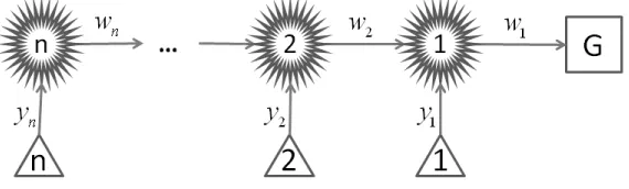
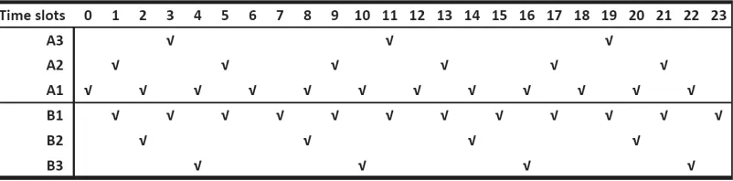
In this section, we study a chain network where each node has at most one adjacent node from which it receives data. Observe that since local clients each require only one data unit to be transfered in each cycle, they can be fitted into an available time slot without violating the perfect periodic nature of the schedule. It is therefore convenient to have a simple diagrammatic representation of the multiple local clients of a node. We use a triangle node for this purpose, and index the nodes by depth from the gateway, as depicted in Figure 1.

Figure 1: A network with the chain structure.

Lemma 2. A chain network has an optimal PPS with q1 = 2 or 3.

Proof. Suppose that the Lemma does not hold. Then there exist an optimal solution withq₁′ ≥4 and periodicityT′,say, for whichT′ ≥4w1 by condition

(5). We now construct a new solution by letting qj = 3 for j = 1, . . . , n, and

τ2h−1 = 0 for h= 1, . . . ,⌈n/2⌉ and τ2h = 1 for h= 1, . . . ,⌊n/2⌋.

Conditions (1) and (2) are trivially satisfied forj =nsinceLn ={ln}has

only one element. For j = 1, . . . , n−1, Lj = {lj, lj+1} and gcd(qj, qj+1) =

3. Thus, for j ≤ n −1, condition (1) is satisfied by Lemma 1 since τj ̸≡

τj+1 mod 3, and condition (2) is satisfied since

∑

j′∈Lj

1

qj′

= 1

qj

+ 1

qj+1

= 1 3 +

1 3 < 1.

Condition (3) is trivially satisfied since G has only one element. Moreover,

T = 3w1 satisfies condition (4) since qj = 3 for allj, and condition (5) since

T = 3w1 =w1qj ≥wjqj for all j. Moreover, condition (6) is satisfied since

T



1− ∑

j′∈Lj

1

qj′



 > 3yj

(

1− 1

qj −

1

qj+1

)

= 3yj

(

1− 1 3−

1 3

)

and T = 3w1 ≥ 3wj >3yj for all j. Therefore, the new solution is feasible

and has T = 3w1 < T′, providing the required contradiction.

Theorem 1. For a chain network with two or more nodes and y1 ≤w2, an

optimal PPS is provided by

q = (q1, q2, . . . , qn) =

{

(2,4,4, . . . ,4) if y1 ≥w2/3

(3,3,3, . . . ,3) if y1 < w2/3 τ = (τ1, τ2, . . . , τn) = (0,1,0,1, . . . ,0,1),

with

T =

{

4w2 if 3w1 ≥4w2

3w1 if 3w1 <4w2

Proof. By Lemma 2, there are two cases to consider: q1 = 2 and q1 = 3.

Suppose that q1 = 2. Due to the local transmission to the node 1, we

have that q2 ≥ 3. Since q1 and q2 cannot be coprime, q2 ≥ 4 and hence T ≥4w2 by condition (5). A feasible solution withT = 4w2 can be obtained

by setting q1 = 2 and qj = 4 for j = 2, . . . , n, and τ2h−1 = 0 for h =

1, . . . ,⌈n/2⌉ and τ2h = 1 for h = 1, . . . ,⌊n/2⌋. Then, τj and τj+1 for j =

1, . . . , n −1 satisfy condition (1) by Lemma 1 since Lj = {lj, lj+1} and τj ̸≡τj+1 modgcd(qj, qj+1). Condition (2) is satisfied because

∑

j′∈Lj

1

qj′

= 1

qj

+ 1

qj+1 ≤

1 2 +

1

4 < 1 for all j.

Condition (3) is trivially satisfied sinceGhas only one element. Condition (4) is satisfied becauseT = 4w2 andlcm(q1, . . . , qn) = 4. Since 2w2 ≥w2+y1 = w1, we have that T = 4w2 ≥ 2w1 ≥ w1q1 and T = 4w2 ≥ 4wj = wjqj for

j = 2, . . . , n, satisfying condition (5). Moreover, condition (6) is satisfied since T = 4w2 ≥4yj and

T



1− ∑

j′∈Lj

1

qj′



 _≥ 4yj

(

1− 1

qj

− 1

qj+1

)

≥ 4yj

(

1−1 2 −

1 4

)

= yj for all j.

Therefore, the solution is feasible and has T = 4w2.

We now suppose thatq1 = 3. Then,T ≥3w1 by condition (5). A feasible

τ2h−1 = 0 forh = 1, . . . ,⌈n/2⌉ and τ2h = 1 for h= 1, . . . ,⌊n/2⌋. τj and τj+1

for j = 1, . . . , n−1 satisfy condition (1) by Lemma 1 since Lj ={lj, lj+1}

and τj ̸≡τj+1 modgcd(qj, qj+1). Condition (2) is satisfied because

∑

j′∈Lj

1

qj′

= 1

qj

+ 1

qj+1

= 1 3+

1

3 < 1 for all j.

Condition (3) is trivially satisfied sinceGhas only one element. Observe that

T = 3w1satisfies conditions (4) - (6) as follows: condition (4) is satisfied since qj = 3 for all j and condition (5) is satisfied since T = 3w1 = w1qj ≥ wjqj

for all j. Moreover, condition (6) is satisfied sinceT = 3w1 ≥3wj >3yj and

T



1− ∑

j′∈Lj

1

qj′



 > 3yj

(

1− 1

qj −

1

qj+1

)

= 3yj

(

1− 1 3−

1 3

)

= yj for all j.

Therefore, the new solution is feasible and has T = 3w1. Consequently, if

y1 ≤ w2, then there exits an optimal solution having T = min{3w1, 4w2}.

Observe that nodes at depth 3 onward have no explicit effect on the T. However, reducing the chain to depth 1 reduces T to 2w1.

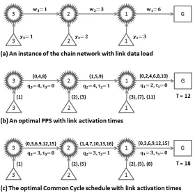
Example 1. Consider a chain network of depth 3 with input data y1 = 3, y2 = 2 and y3 = 1 as shown Figure 2 (a). By Theorem 1, an optimal

PPS is provided by q = (q1, q2, q3) = (2,4,4), τ = (τ1, τ2, τ3) = (0,1,0) and T = min{3w1,4w2} = 12. The corresponding full set of time slots in which

links are activated within each full cycle is indicated in Figure 2 (b). Each local client’s link is activated once in every full cycle of length 12.

Now consider how a standard routing protocol using a Common Cycle of periodicity qC _{would schedule data transfer. It requires q}C _{≥ 3, to satisfy}

condition (2) since node 2 has three links. SinceTC ≥_qC_w

1,qC = 3 provides

the optimal Common Cycle schedule. Thus, for Example 1, TC = 3∗6 = 18 compared withT∗ = 12 andTC_/T∗ _{= 3/2. More generally, when 3w}

1 ≥4w2,

from Theorem 1,

TC

T∗ =

3w1

4w2

= 3(2w2−(w2−y1)) 4w2

= 3 2−

3

Figure 2: The chain network and its schedules for Example 1.

Theorem 2. For a chain network, perfect periodic schedule accommodates up to 50% more capacity than the standard Common Cycle approach.

4. Binary tree network with a single link to the Gateway

When a routing tree has multiple Mesh nodes adjacent to the Gateway, the PPS problem is NP-hard [4]. We study the special case of a routing tree in which each mesh node has at most two incoming access links, namely a

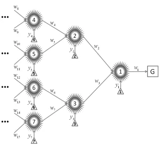
binary treenetwork. For ease of analysis, we first study the case with only one Mesh node adjacent to the Gateway, defined as half binary tree network. We then extend this result to the case where there are two Mesh nodes adjacent to the Gateway in the next section.

Figure 3: The structure of a half binary tree.

transmission requirement, eg. w2 ≥ w3. In addition, we may refer to the two incoming links at node j as j1 and j2 where wj1 ≥ wj2 by convention.

We assume throughout that the input data flow rates is not too large at any single node. More precisely, yj ≤wj2 for all j.

Our approach is to identify a limited number of possible dominant so-lutions for half of a binary (sub)tree before proceeding to consider optimal solutions for whole binary tree. It is sufficient to consider three classes of feasible schedules, one for each values of q1, namely S2 for q1 = 2, S3 for q1 = 3 and Sa for q1 =a and a ≥4.

4.1. Case of base periodicity 2

Lemma 3. For any two integers a and b, the schedule S2(a, b) where a≥2

q1 = 2, τ1 = 0, q2 = 2a, τ2 = 1, q3 = 2ab, τ3 = 3,

qj1 = qj, τj1 = R(τj + 1,2a) for j = 2, . . . , n,

qj2 = qj, τj2 = R(τj + 3,2a) for j = 2, . . . , n,

is feasible with T ≥max{2aw2,2abw3} and 2ab|T.

Proof. Observe that τ1 ̸≡ τ2 mod gcd(q1, q2), τ2 ̸≡ τ3 mod gcd(q2, q3)

and τ3 ̸≡ τ1 mod gcd(q3, q1). Moreover, τj′ ̸≡ τj′′ mod gcd(qj′, qj′′) forj′ ̸=

j′′ and j′, j′′∈ Lj for j = 2, . . . , nby construction. Therefore, τj, τj1 and τj2

satisfy condition (1) by Lemma 1 for all j. Moreover, for allj

∑

j′∈Lj

1

qj′

= 1

qj

+ 1

qj1

+ 1

qj2

≤ 1

2 + 1 2a +

1 2ab ≤

1 2+

1 4+

1 6 < 1, ensuring that condition (2) is satisfied. Condition (3) is trivially satisfied since G has only one element. Thus, S2(a, b) is feasible. Conditions (4) and

(5) mean that 2ab|T and T ≥max{2w1,2aw2,2abw3}= max{2aw2,2abw3}

by Appendix A. Then, condition (6) is satisfied since

T

(

1− ∑

j′∈L1

1

qj′

)

≥2abw3

(

1− 1 2 −

1 2a −

1 2ab

)

= ((a−1)b−1)w3 ≥ y1

and

T



1− ∑

j′∈Lj

1

qj′



 _≥ 2aw2

(

1− 1 2a −

1 2a −

1 2a

)

= (2a−3)w2 ≥ yj forj = 2, . . . , n.

Lemma 4. For a half binary tree structure with canonical indexing, ifq1 = 2

and q2 = 4in a PPS, then q3 must be a multiple of4 in any feasible solution.

Proof. Suppose otherwise, then there is a feasible PPS solution withq1 = 2, q2 = 4 and q3 is of the form 4a+ 2, sinceq3 is a multiple of 2 by Corollary 1.

Thus, gcd(q1, q2) = gcd(q2, q3) = gcd(q3, q1) = 2, and hence τ1 ̸≡ τ2 mod 2,

τ2 ̸≡τ3 mod 2 and τ3 ̸≡τ1 mod 2. This implies that the values τ1, τ2 and τ3

Lemma 5. For a network containing a half binary subtree with q1 = 2, there

exists an optimal PPS having one of following forms with the corresponding constraints on the value of T:

S2(2, a) for a≥2, with T ≥4amax

{⌈_w

2 a

⌉

, w3

}

and 4a|T,

or

S2(a,1) for a ≥3, with T ≥2aw2 and 2a|T.

Proof. Take a feasible PPS for a half binary tree with q1 = 2 and the

corresponding T. Both q2 and q3 have to be a multiple of 2 since q1, q2 and q3 cannot be pairwise coprime by Corollary 1. Due to transmissions of the

link 3, ie. w3 > 0, we have that q2 ≥ 4. We consider the cases q2 = 4 and q2 = 2a fora ≥3, separately.

Suppose that q2 = 4. Note that q3 must be a multiple of 4, q3 = 4b

say, by Lemma 4, and b ≥ 2 to allow time for the local transmissions of the node 1, y1. Conditions (4) and (5) imply that T is a multiple of 4b and

that T ≥ max{2w1,4w2,4bw3} = max{4w2,4bw3} by Appendix A. Thus, T ≥4bmax{⌈w2/b⌉, w3} and 4b|T. Observe that both these conditions are

precisely the constraints on the value of T in S2(2, b) from Lemma 3.

Now suppose that q2 = 2a and a ≥ 3. Since 3w2 ≥ w1 and a ≥ 3,

conditions (4) and (5) imply that T ≥ max{2w1,2aw2} = 2aw2 and 2a|T.

Observe that this condition is precisely the constraints on the value of T in

S2(a,1) from Lemma 3.

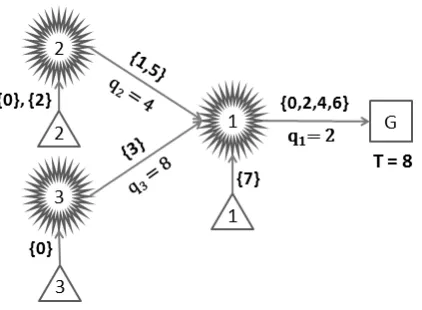
Example 2. Consider a half binary tree network of depth 2 with input data

y1 = 1, y2 = 2 and y3 = 1. Then, w1 = 4, w2 = 2 and w3 = 1. By Lemma

5, an optimal PPS with q1 = 2 is provided by q = (q1, q2, q3) = (2,4,8), τ =

(τ1, τ2, τ3) = (0,1,3) and T = 8 max{⌈w2/2⌉, w3} = 8. The corresponding

full set of time slots in which links are activated within each full cycle is indicated in Figure 4. Each local client’s link is activated once in every full cycle of length 8.

4.2. Case of base periodicity 3

Lemma 6. For a network containing a half binary subtree with q1 = 3,

Figure 4: An optimal PPS with q1 = 2 for Example 2, specified by its link activation times.

constraints on the value of T: S3(a) for a≥2 with q2r = 3 for r= 0, . . . ,⌊log₂n⌋,

qj = 3a for all other j’s,

τ1 = 0,

τj1 = R(τj+ 1,3) for all j,

τj2 = R(τj+ 2,3) for all j,

which has

T ≥3amax

{⌈_w

1 a

⌉

,wb

}

and 3a|T, where wb= max{w2r₊₁ :r= 1, . . . ,⌊log₂n⌋}.

Proof. We first show thatS3(a) fora≥2 is feasible, withT ≥3amax{⌈w1/a⌉,wb}

and 3a|T, where wb= max{w2r₊₁ :r= 1, . . . ,⌊log₂n⌋}. Observe thatτ_j,τ_j 1

and τj2 satisfy condition (1) by Lemma 1 for all j. Condition (2) is satisfied

since a ≥2 and

∑

j′∈Lj

1

qj′

= 1

qj

+ 1

qj1

+ 1

qj2

≤ 1

3+ 1 3+

1

3a < 1 for all j.

Condition (3) is trivially satisfied sinceGhas only one element. Thus,S3(a) is

feasible. Observe that wb= max{w2r₊₁ : 0≤r≤ ⌊log₂n⌋}= max_j∈J\J 1{wj},

whereJ ={1, . . . , n}andJ1 ={2r : 0≤r ≤ ⌊log2n⌋}, because a star-nodej

1 : 0 ≤ r ≤ ⌊log₂n⌋}. Thus, condition (5) imposes that T ≥ max{wjqj} =

max{3 maxj∈J1{wj},3amaxj∈J\J1{wj}

}

= max{3w1,3awb}. Condition (4)

imposes that T is divisible by 3a and strengthens the bound on T to T ≥

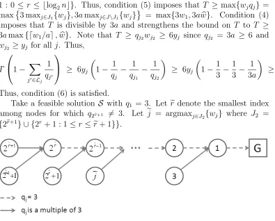
3amax{⌈w1/a⌉,wb}. Note that T ≥ qj2wj2 ≥ 6yj since qj2 = 3a ≥ 6 and

wj2 ≥yj for all j. Thus,

T



1− ∑

j′∈Lj

1

qj′



 _≥ 6yj

(

1− 1

qj −

1

qj1

− 1

qj2

)

≥ 6yj

(

1− 1 3 −

1 3 −

1 3a

)

≥ yj for all j.

Thus, condition (6) is satisfied.

Take a feasible solution S with q1 = 3. Let redenote the smallest index

among nodes for which q₂er+1 ̸= 3. Let ej = argmax_j∈J

2{wj} where J2 = {2er+1_{} ∪ {2}r_{+ 1 : 1≤r ≤er+ 1}}.}

Figure 5: Illustration ofJ2 subnetwork part of a feasible solution withq1= 3.

Since qj = 3 for j ∈ {2r : 0≤r≤re}, we have that qj for j ∈J2 are each

multiples of 3 by Corollary 1. Since qj >3 forj ∈J2 to accommodate local

transmission at star-node 2r _{for r = 0, . . . ,er, we have that q}

ej is of the form

3a for some integera and a≥2. Thus, T(S) is constrained by condition (4) to have 3a|T(S) and by condition (5) to have T(S) ≥ max{3w1,3awe_j} =

3amax{⌈w1/a⌉, we_j}. Sincew2er₊₁ ≥w₂j₊₁forj ≥er+2, from the definition of

ej, we have thatw_ej ≥max{w2r₊₁ : 0≤r≤ ⌊log₂n⌋}=wb. Therefore,T(S)≥

3amax{⌈w1/a⌉, wej} ≥ 3amax{⌈w1/a⌉,wb} = T(S3(a)), which implies that

there exists an optimal PPS with the form of S3(a).

4.3. Optimal solutions a for half-binary tree

Theorem 3. For a half binary tree, there is an optimal PPS of one of the following forms:

S2(2,2) with T = 8 max{⌈w2/2⌉, w3},

S2(3,1) with T = 6w2,

S3(2) with T = 6⌈w1/2⌉,

and if there exists an integer a such that a|w2 and 3≤a < w2/w3,

S2(2, a) with T = 4w2,

and if there exists an integer a such that a|w1 and 3≤a < w1/wb,

S3(a) with T = 3w1

where wb= max{w2r₊₁ :r= 1, . . . ,⌊log₂n⌋}.

Proof. There are three cases to consider: q1 = 2, q1 = 3 and q1 ≥4.

When q1 = 2, by Lemma 5, it is sufficient to consider only schedules

S2(2, a) for a≥2 withT = 4amax{⌈w2/a⌉, w3} and S2(a,1) fora ≥3 with T = 2aw2. By Appendix B for T /4, T is mimimized to

{

4w2 if there exists an integer a such that a|w2 and 3≤a < w2/w3,

8 max{⌈w2/2⌉, w3} otherwise,

by S2(2, a) and S2(2,2), respectively. Moreover, S2(a,1) for a ≥ 3 achieves

the smallest T value by settinga= 3 to give T = 6w2.

When q1 = 3, by Lemma 6, it is sufficient to consider schedules of the

form S3(a) for a ≥ 2 with T = 3amax{⌈w1/a⌉,wb}. Note that w1 ≥ 2wb

since w1 ≥ w2r−1 = w₂r₊₁ +w₂r +y₂r−1 > w₂r₊₁ +w₂r ≥ 2w₂r₊₁, because

w2r ≥ w₂r₊₁ for r = 1, . . . ,⌊log₂n⌋. Thus, Appendix B may be applied to

T /3 to give the smallest value of T

{

3w1 if there exists an integer a such that a|w1 and 3≤a < w1/wb, 6⌈w1/2⌉ otherwise,

from S3(a) and S3(2) respectively.

Now consider a feasible solution with q1 ≥ 4, from condition (5), T ≥ q1w1 ≥ 4w1 ≥ 3(w1 + 1)≥ 6⌈w1/2⌉ since w1 ≥ 3. Thus, any solution with q1 ≥4 is dominated by the solution S3(2).

Lemma 7. For a network containing a half binary subtree with q1 =a≥4,

there exists an optimal PPS, Sa, having the following form

qj = a for j = 1, . . . , n,

τ1 = 0,

τj1 = R(τj+ 1, a) for all j,

τj2 = R(τj+ 2, a) for all j,

with periodicity T constrained by the two conditions

T ≥w1a and a|T.

Proof. We first show that the solutions Sa for a ≥ 4 is feasible. Observe

that τj, τj1 and τj2 satisfy condition (1) by Lemma 1 for all j. Condition

(2) is satisfied since

∑

j′∈Lj

1

qj′ ≤

1

qj

+ 1

qj1

+ 1

qj2

≤ 1

4 + 1 4 +

1

4 < 1 for for all j.

Condition (3) is trivially satisfied sinceGhas only one element. Observe that

a|T and T ≥w1a are precisely conditions (4) and (5). Moreover, condition

(6) is satisfied since

T



1− ∑

j′∈Lj

1

qj′



 _≥ 4w1

(

1− 1 4−

1 4 −

1 4

)

= w1 ≥ yj for for all j.

Take a feasible PPS withq1 =a and a≥4. Then, by conditions (4) and

(5), a|T and T ≥ w1a. Observe that both these conditions are precisely

the constraints on the value of T inSa.

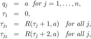
5. Binary routing tree network: properties of an optimal schedule

We now extend the results for the half binary tree to the whole binary tree. Figure 7 depicts the structure of the whole binary tree which can be decomposed into two half binary trees. We index the two half binary trees independently using canonical indexing, and assume without loss of generality that wA1 ≥wB1. We assume throughout that the input data flow

k = A, B and all non-peripheral nodes j (j2 being undefined for peripheral

nodes). Let nA and nB denote the numbers of star-nodes in the left-hand

side half binary tree and the right-hand side half binary tree, respectively, where n = nA+nB. We define a composite function ◦ for combining two

feasible schedules, one for each of the two for two half binary trees, into a single schedule for the whole binary tree. The composite periodicity vector

q = q

A ◦qB leaves the periodicities unchanged, while τ = τA ◦τB retain

the relative start time within each subschedule but shift the timing for one tree by one time-unit to avoid overlap at the gateway. Thus, τAj ← τAj for

j = 1, . . . , nA and τBj ← R(τBj + 1, qBj) for j = 1, . . . , nB. Observe that

feasibility of the composite tree SA◦ SB is inherited from feasibility of SA

and SB independently and conditions (1) and (3) at the gateway. Condition

(1) holds by Corollary 1 because |τA1 −τB1 | = 1 and gcd(qA1, qB1) ≥ 2.

Condition (3) holds because qA1 ≥2, qB1 ≥ 2 and yG = 0. Moreover, there

are no additional constraints on T other than those imposed by subtrees SA

andSB, since (4) - (6) are edge conditions and the single condition associated

with the new gateway node, condition (6), is automatically satisfied since it is assumed to have no direct input, yG= 0.

We find an optimal solution for the whole binary tree by coordinating limited number of feasible solutions for the half binary tree.

Figure 6: The structure of a binary tree.

Proof. Suppose that there exists an optimal schedule S withqA1 ≥4. From

condition (5), the solution hasT(S) ≥ 4wA1 ≥ 3(wA1+1) becausewA1 ≥3.

Note that S3(2)◦ S3(2) has 6|T and T ≥ max{3wA1,3wB1,6wA3,6wB3} =

3wA1 because wB1 ≤ wA1, 2wA3 < wA2 +wA3 +yA1 = wA1, and 2wB3 < wB2+wB3+yB1 =wB1. Thus, T(S3(2)◦ S3(2)) = 6⌈wA1/2⌉ ≤ 3(wA1 + 1).

Therefore, S is dominated by S3(2)◦ S3(2), providing the required

contra-diction.

Lemma 9. For any instance of the whole binary tree network, there exists an optimal solution with qA1 ≤3 and qB1 ≤4.

Proof. Take an optimal schedule S =SA◦ SB. Without loss of generality,

we assume that τA1 = 0. From Lemma 8 qA1 = 2 or 3. Now suppose that

the Lemma does not hold, and thus qB1 ≥5, and henceqB1 ≥6 by Corollary

1 applied to the gateway node. Let a = qA1 and b = qB1. Construct new

solution S′ =SA◦ SB′ by setting

q′_Aj = qAj for j = 1, . . . , nA,

q_B′ ₁ = a,

q_Bj′ = b forj = 2, . . . , nB,

τ_Aj′ = τAj for j = 1, . . . , nA,

τ_B′₁ = 1, τ_B′₂ = 0, τ_B′₃ = 2, τ_Bj′

1 = R(τ

′

Bj + 1, b) forj = 2, . . . , nB,

τ_Bj′ ₂ = R(τ_Bj′ + 2, b) forj = 2, . . . , nB.

Observe that τ_Bj′ , τ_Bj′

1 and τ

′

Bj2 satisfy condition (1) by Lemma 1 for j =

1, . . . nB. Condition (2) is satisfied because

∑

j′∈LBj

1

qj′

= 1

qBj

+ 1

qBj1

+ 1

qBj2

≤ 1

a+

1

b+

1

b ≤

1 2+

1 6+

1 6 =

5

6 < 1 forj = 1, . . . , nB. Condition (3) holds because q′_A1 ≥ 2, q_B′ ₁ ≥ 2 and yG = 0. Thus, S′ is

T(S). Condition (4) is satisfied because T(S) is divisible by both qA1 = a

and qB1 =b. Condition (5) is satisfied because

max{wAjqAj′ , wBjqBj′ } = max{wA1q′A1, max

j∈{2,...,nA}

{wAjqAj′ }, wB1q′B1, max

j∈{2,...,nB}

{wBjqBj′ }}

= max{wA1a, max

j∈{2,...,nA}

{wAjqAj′ }, wB1a, max

j∈{2,...,nB}

{bwBj}}

≤ max{wA1a, max

j∈{2,...,nA}

{wAjqAj}, wB1b}

= max{wA1qA1, max

j∈{2,...,nA}

{wAjqAj}, wB1qB1}

≤ T(S).

Note that q_B′ ₁ ≥ 2 and q_Bj′ ≥ 6 for j = 2, . . . , nB. Moreover, since T(S) ≥

q_Bj′ wBj =bwBj ≥bwBj2 ≥6yBj forj = 1, . . . , nB,

T(S)



1− ∑

j′∈LBj

1

qj′



 _≥ 6yBj

(

1− 5 6

)

≥ yBj,

and thus, condition (6) is satisfied.

From Lemmas 8 and 9, it is sufficient to consider only solutions with

qA1 = 2,3 andqB1 = 2,3,4. Moreover, since qA1 and qB1 cannot be co-prime

from Corollary 1, when qA1 = 2 the value of qB1 is 2 or 4, and when qA1 = 3 qB1 is 3. We now consider each of these three cases in turn.

Lemma 10. Any feasible PPS for a whole binary tree with qA1 = 3 is

domi-nated by a solutionS3(a)◦S3(a)withT = 3amax{⌈wA1/a⌉,wb}for some

in-teger a≥2, where wb= max{wk(2r₊₁₎ :r= 1, . . . ,⌊log₂n_k⌋ and k =A, B

}

.

Proof. Take a feasible schedule SA ◦ SB with qA1 = 3. As observed

above, qB1 = 3 from Corollary 1. Thus, by Lemma 6, SA and SB are

dom-inated by S3(aA) and S3(aB), respectively, where 3aA | T, 3aB | T, T ≥

3aAmax{⌈wA1/aA⌉,wbA} and T ≥ 3aBmax{⌈wB1/aB⌉,wbB} where wbA and

b

wB are defined in Lemma 6. The rest of the proof follows by setting a=aA

if wbA≥wbB anda =aB ifwbA <wbB, sincewA1 ≥wB1 and wb= max{wbA,wbB}

as defined above.

Lemma 11. Any feasible PPS for a whole binary tree with qA1 = qB1 = 2

is dominated by one of the following solutions S2(2, a)◦ S2(2, a) for some

integer a ≥2 with

T = 4amax

{⌈_w

A2 a

⌉

, wA3,

⌈_w

B2 a

⌉

, wB3

}

S2(2,2)◦ S2(3,1) with

T = 24 max

{⌈_w A2 6 ⌉ , ⌈_w A3 3 ⌉ , ⌈_w B2 4 ⌉} ,

S2(2, a)◦ S2(a,1)and a≥3 with T = 4amax{

⌈_w

A2 a

⌉

, wA3,

⌈_w

B2

2

⌉

},

S2(3,1)◦ S2(2,2) with

T = 24 max

{⌈_w A2 4 ⌉ , ⌈_w B2 6 ⌉ , ⌈_w B3 3 ⌉} ,

S2(a,1)◦ S2(2, a) and a≥3 with T = 4amax{

⌈_w A2 2 ⌉ , ⌈_w B2 a ⌉

, wB3},

S2(3,1)◦ S2(3,1) with

T = 6 max{wA2, wB2}.

Proof. From the result for a network containing a half binary subtree in Lemma 5, it is sufficient to consider all combinations of SA = S2(2, a) for a≥2 orSA=S2(a,1) fora≥3 and SB =S2(2, b) for b≥2 orSB =S2(b,1)

for b ≥3. We consider these cases separately.

Case 1: SA=S2(2, a) fora≥2 and SB =S2(2, b) for b≥2.

By Lemma 5, we have that 4a|T, 4b|T andT ≥4 max{amax{⌈wA2/a⌉, wA3}, bmax{⌈wB2/b⌉, wB3}}.

Thus, an optimal T value is of the form

T ≥4a′max

{⌈_w

A2 a′

⌉

, wA3,

⌈_w

B2 a′

⌉

, wB3

}

,

by setting a′ =a if wA2 > wB2 and a′ =b if wA2 ≤wB2.

Case 2: SA=S2(2, a) fora≥2 and SB =S2(b,1) for b≥3.

We first consider the subcase when a = 2 and b = 3. In this subcase, by Lemma 5, we have that 24|T and T ≥max{4wA2,8wA3,6wB2}. Thus,

T = 24 max

We now consider the subcase when a = 2 and b ≥ 4. By Lemma 5, we have that 8|T, 2b|T and

T ≥ max{4wA2,8wA3,2bwB2}

≥ max{4wA2,8wA3,4wB2,8wB3}

= 8 max

{⌈_w

A2

2

⌉

, wA3,

⌈_w

B2

2

⌉

, wB3

}

= T(S2(2,2)◦ S2(2,2)),

implying that in this subcase, any solution can be dominated by a solution

S2(2,2)◦ S2(2,2).

Finally, we consider the subcase whena≥3 andb≥3. Then, by Lemma 5, we have that 4a|T, 2b|T and T ≥ max{4wA2,4awA3,2bwB2}. Thus, an

optimal T value is of the form

T = 4a′max{

⌈_w

A2 a′

⌉

, wA3,

⌈_w

B2

2

⌉

},

by setting a′ =a if 4wA3 >2wB3 and a′ =b if 4wA3 ≤2wB3.

Case 3: SA=S2(a,1) for a≥3 and SB =S2(2, b) for b≥2

This case is similar to Case 2 but with the roles ofa and breversed. Ifa = 3 and b = 2,

T = 24 max

{⌈_w

A2

4

⌉

,

⌈_w

A3

6

⌉

,

⌈_w

B2

3

⌉}

.

If a≥3 and b≥3, then

T = 4a′max{

⌈_w

A2

2

⌉

,

⌈_w

B2 a′

⌉

, wB3},

where a′ =a if 2wA2 >4wB3 and a′ =b if 2wA2 ≤4wB3.

Case 4: SA=S2(a,1) for a≥3 and SB =S2(b,1) for b≥3.

by Lemma 5, we have that 2a|T, 2b|T and

T ≥max{2awA2,2bwB2} ≥6 max{wA2, wB2}=T(S2(3,1)◦ S2(3,1)).

Thus, the solution is dominated by a solution S2(3,1)◦ S2(3,1).

Lemma 12. Any feasible PPS for a whole binary tree with qA1 = 2 and qB1 = 4, which is not dominated by a solution with qA1 = qB1 = 2, is

S2(2, a)◦ S4 for some integer a≥3 with T = 4amax

{⌈_w

A2 a

⌉

, wA3,

⌈_w

B1 a

⌉}

,

S2(3,1)◦ S4 with

T = 12 max

{⌈_w A2 2 ⌉ , ⌈_w B1 3 ⌉} ,

Proof. Note that any feasible PPS SA◦ SB with qB1 = 4 is dominated by

a solution with SB =S4 by Lemma 7. SinceqA1 = 2, by Lemma 5 there are

two cases to consider: SA=S2(2, a) fora≥2, and SA=S2(a,1) for a≥3.

Case 1: S2(2, a)◦ S4 for a≥2

By Lemmas 5 and 7, we have that 4a|T and T ≥max{4wA2,4awA3,4wB1}.

If a= 2, then

T = max{4wA2,8wA3,4wB1}

= 8 max

{⌈_w

A2

2

⌉

, wA3,

⌈_w B1 2 ⌉} ≥ max {⌈_w A2 2 ⌉

, wA3,

⌈_w

B2

2

⌉

, wB3

}

= T(S2(2,2)◦ S2(2,2)),

implying that the solution is dominated by S2(2,2)◦ S2(2,2). Ifa ≥3, then T = 4amax

{⌈_w

A2 a

⌉

, wA3,

⌈_w

B1 a

⌉}

.

Case 2: S2(a,1)◦ S4 for a≥3

By Lemmas 5 and 7, conditions onT are 4|T, 2a|T andT ≥max{2awA2,4wB1}.

Thus, when a = 3,

T = 12 max

{⌈_w A2 2 ⌉ , ⌈_w B1 3 ⌉} .

Now take a ≥ 4 and compare S2(a,1)◦ S4 and its time frame T with the

alternative schedule S2(2, a)◦ S4. The alternative schedule is feasible with q_A′ ₂ = 4 < 2a = qA2, q′Aj =qAj = 2a or 4, for all other values of j, and thus

4|T′, 2a|T′ andq′_Aj ≤qAj for all values ofj.Hence,T′ ≤T and S2(a,1)◦ S4

6. Binary routing tree network: optimal algorithm

In the previous section we classified the forms which we need to consider for an optimal PPS for a binary tree in Lemmas 10 to 12. Several of these forms are parameterised by the variable aand it is therefore useful to reduce the range of potential values ofa, which we now do in the following Lemma. Algorithm OptPPS and Theorem 4 then draws these results together. The efficiency of the optimisation algorithm OptPPS is considered at the end of the section, along with its effectiveness relative to the standard round robin, Common Cycle, schedule.

Lemma 13. For a binary tree network, PPS of the following formsS2(2, a)◦

S2(a,1), and S2(2, a)◦ S2(2, a), S2(2, a)◦ S4, and S2(a,1)◦ S2(2, a), may be

optimal only for values of a less than 8, 8, 8, and 5, respectively.

Proof. Observe that we may restrict attention to the case T < 3(wA1 + 1)

since S3(2) ◦ S3(2) has T = 6⌈wA1/2⌉ ≤ 3 (wA1+ 1). In addition, it is

sufficient to consider a solution withqA1 = 2 only ifwA2 <9wA3. To see this

take an instance with wA2 ≥9wA3 and a PPS solution with qA1 = 2. Then, qA2 ≥ 4 by Lemma 4, and hence, by condition (5) and the assumption that yA1 ≤wA3,

T ≥4wA2 ≥3wA2+ 9wA3 ≥3wA2 + 3 (wA3+yA1+ 1)≥3 (wA1+ 1),

providing the required contradiction.

Consider a solution with one of the following forms, S2(2, a)◦ S2(a,1),

S2(2, a)◦ S2(2, a) and S2(2, a)◦ S4. In order for one of these solutions to be

optimal, it must hold that 4awA3 ≤T <3(wA1+ 1), since qA3 = 4a. Thus, a < 3(wA1+ 1)

4wA3

= 3(wA2+wA3+yA1+ 1) 4wA3

≤ 3(wA2+ 3wA3)

4wA3

<9,

since we are restricting attention to instances for which wA2 < 9wA3. Now

consider a solution in the form of S2(a,1)◦ S2(2, a). It has qA2 = 2a and

therefore 2awA2 < T ≤3(wA1+ 1). Hence, a < 3(wA1+ 1)

2wA2

= 3(wA2+wA3+yA1 + 1)

2wA2 ≤

3(4wA2)

2wA2 ≤

6,

Algorithm OptPPS

Find the minimum T value amongst the following forms, and output in ad-dition a corresponding schedule:

S3(2)◦ S3(2) with T = 6⌈wA1/2⌉;

S3(a)◦ S3(a) with T = 3wA1 for 3≤a, a|wA1, and a < wA1/wb

where wb= max{wk(2r₊₁₎ :r= 1, . . . ,⌊log₂n_k⌋ and k=A, B

}

;

S2(2,2)◦ S2(2,2) with T = 8 max{⌈wA2/2⌉, wA3,⌈wB2/2⌉, wB3};

S2(2,2)◦ S2(3,1) with T = 24 max{⌈wA2/6⌉,⌈wA3/3⌉,⌈wB2/4⌉};

S2(2, a)◦ S2(a,1) with T = 4amax{⌈wA2/a⌉, wA3,⌈wB2/2⌉}for 3≤a≤8;

S2(3,1)◦ S2(2,2) with T = 24 max{⌈wA2/4⌉,⌈wB2/6⌉,⌈wB3/3⌉};

S2(a,1)◦ S2(2, a) with T = 4amax{⌈wA2/2⌉,⌈wB2/a⌉, wB3} for 3≤a ≤5;

S2(3,1)◦ S2(3,1) with T = 6 max{wA2, wB2};

S2(2, a)◦ S2(2, a) with T = 4 max{wA2, wB2} for 3≤a≤8, a| max{wA2, wB2}, and a <max{wA2, wB2}/max{wA3, wB3};

S2(2, a)◦ S4 with T = 4amax{⌈wA2/a⌉, wA3,⌈wB1/a⌉} for 3≤a≤8;

S2(3,1)◦ S4 with T = 12 max{⌈wA2/2⌉,⌈wB1/3⌉}.

Theorem 4. For a whole binary tree, Algorithm OptPPS provides an opti-mal perfect periodic schedule.

Proof. We have established in the previous section that only solutions with

qA1 = qB1 = 3 and qA1 = 2 with qB1 = 2 or 4, described in Lemmas 10, 11

and 12 need be considered.

When qA1 = qB1 = 3 potential optimal solutions are of the form S3(a)◦

S3(a) with periodicity T = 3amax{⌈wA1/a⌉,wb} from Lemma 10. Now

wA1 ≥ 2w,b since wA1 ≥ wB1 and wk1 ≥ wk2r−1 = w_k2r₊₁+w_k2r +y_k2r−1 >

wk2r₊₁+w_k2r ≥2w_k2r₊₁becausew_k2r ≥w_k2r₊₁from the indexing convention,

for r = 1, . . . ,⌊log₂nk⌋ and k = A, B. Hence, ⌈wA1/2⌉ ≥ wb and from the

result in Appendix B applied to T /3, for a≥2

T =

{

3wA1 if there exists an integer a such thata|wA1 and 3≤a < wA1/wb,

6⌈wA1/2⌉ otherwise,

The solutionS2(2, a)◦ S2(2, a) for a≥2 has

T =

  

4 max{wA2, wB2} if there exists an integer a such that a| max{wA2, wB2}

and 3≤a <max{wA2, wB2}/max{wA3, wB3},

8 max{⌈wA2/2⌉, wA3,⌈wB2/2⌉, wB3} otherwise,

from Lemma 11 and Appendix B. The list of solutions from Lemmas 11 combined with the upper limit on the value of a is given in Lemma 13, thus give rise to the third to the ninth solution forms. The last two forms arise from Lemma 12, with additional restrictions on the range of a imposed by Lemma 13.

Observe that the eleven expressions considered by Algorithm OptPPS as having potentially minimum values for the time frame, T, are each closed form, and that only the second expression may need evaluating more than 8 times. It is sufficient to consider the second expression only for values of

a no greater than √wA1. The second and ninth expressions involve prime

factorisation of an integer no greater than wA1. While factorisation is N P

-hard in general, it can be performed quickly for any integer up to 40 digits long [29]. Since wA1 represents the total number of peripheral clients in the

network, an optimal PPS for a full binary tree network can, in practice, be found in polynomial time.

Observe that if the value ofwA1were to be too large for prime factorisation

by the available software, then a potential optimal solution S3(a) ◦ S3(a)

with value T = 3wA1 might be missed. However, the solution found by the

algorithm would nonetheless be a (1 + 1/wA1) approximation, by comparison

with the value T = 6⌈wA1/2⌉ forS3(2)◦ S3(2).

Having established the efficiency of our optimal algorithm, we now turn our attention to its effectiveness. The standard approach to perfect periodic scheduling is a Common Cycle, or round robin, schedule and we therefore use this as the benchmark.

Lemma 14. For a whole binary tree, an optimal solution with a common periodicity is S4◦ S4 with periodicity qC = 4 and value TC = 4wA1.

Proof. Since mesh nodes have three access links and one local link, from condition (2), qC ≥ _{4. Thus, from condition (5), T} ≥ _q

A1wA1 = qCwA1 ≥

4wA1. Now the schedule with qC = 4 is S4◦ S4 and it has value T = 4wA1

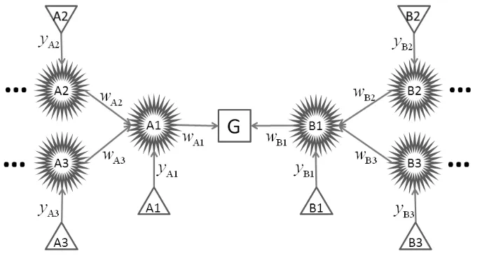
Example 3. Consider a binary tree network of depth 2 with yA1 = 3 yA2 = 6, yA3 = 3, yB1 = 1 yB2 = 3 and yB3 = 1. Then, wA1 = 12 wA2 = 6, wA3 = 3, wB1 = 5 wB2 = 3 and wB3 = 1, and hence TC =

4wA1 = 48 by Lemma 14, while an optimal PPS S2(2,2)◦ S2(3,1) has value T = 24 max{⌈wA2/6⌉,⌈wA3/3⌉,⌈wB2/4⌉} = 24 from algorithm OptPSS,

as shown in Appendix C. Thus, our algorithm doubles the effective capac-ity of the network for this instance of the problem. It can do no better since T∗ ≥ qA1wA1 ≥ 2wA1 and the optimal Common Cycle schedule has T = TC = 4wA1 by Lemma 14, verifying the Theorem below. An optimal

schedule of the above form is presented in Figure 8 for completeness.

Figure 7: An optimal PPS and an optimal Common Cycle schedule for Example 3.

Theorem 5. For any binary tree the application of the optimal PPS algo-rithm provides up to 100% additional capacity over the optimal Common Cycle schedule, i.e.,

TC

Figure 8: The structure of an optimal PPS for Example 3.

7. Computational study

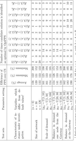
A set of experiments was carried out to explore the behaviour of our algorithm OptPPS. A benchmark dataset of instances was devised to take account of various characteristics: size of the network, using depth of 2, 4 and 6 links from the Gateway node; scale of demand, with maximum user demand up to 10, 50, and 100; and the distribution of demand both within and between the two sides of the binary tree as described below. Local demand is generated randomly from a uniform distribution for each node in the network (other than the Gateway) for 20 instances. The benchmark test suite is included as a supplement to the electronic version of this article. The results of applying OptPPS to the benchmart test suite are reported for each of the data sets in Table 1.

The first section of Table 1 provides the values given in the form of ca-pacity gain compared to default alternative of a, in fact the best, Common Cycle (CS). The second section shows the total number of times a candidate solution achieves the optimal value within each set, and is generally greater than 20 due to multiple optima. The 100% capacity gain of OptPPS over CS, postulated in Theorem 5, is achieved for some of the small instances. However, the maximum value and the spread in capacity gain within a data set reduces as the size of the network increases, with the gain narrowing to within 1% of 33% consistently for networks extending 6 links from the Gateway.

T able 1: The results of the p erformance of OptPPS. T est sets P arameter setting Efficiency of Num b er of times candidate solution is iden tified PPS o v er CS as optimal b y OptPPS Characteristic of in-stance under in v esti-gation V ariables whic h differ from de-fault v alues † Average (%) Minimum (%) Maximum (%) S 3 (2) ◦S 3 (2) S 3 ( a ) ◦S 3 ( a ) S 2 (2 , 2) ◦S 2 (2 , 2) S 2 (2 , 2) ◦S 2 (3 , 1) S 2 (2 ,a ) ◦S 2 ( a, 1) S 2 (3 , 1) ◦S 2 (2 , 2) S 2 ( a, 1) ◦S 2 (2 ,a ) S 2 (3 , 1) ◦S 2 (3 , 1) S 2 (2 ,a ) ◦S 2 (2 ,a ) S 2 (2 ,a ) ◦S 4 S 2 (3 , 1) ◦S 4 Size of net w ork ( n = 6) 156 122 200 3 1 9 2 2 3 4 7 1 2 3 n = 30 139 131 152 6 0 8 4 0 2 1 5 0 0 2 n = 126 133 133 133 20 0 0 0 0 0 0 2 0 0 0 Scale of demand ( yk j ∼ U[1 , 10]) 161 125 190 1 0 14 4 1 2 4 6 0 1 3

ykj

∼ U[1 , 50] 161 133 194 1 0 9 2 0 3 2 9 0 0 3

ykj

∼ U[1 , 100] 154 131 195 4 1 9 5 2 2 3 5 1 1 3 Balance in demand one no de from the Gatew a y ( yk 2 ∼ U[1 , 10]) 154 126 175 1 0 13 3 2 1 0 5 0 1 0

yk2

∼ U[20 , 30] 141 133 153 7 3 14 0 0 0 0 0 5 0 0

yk2

∼ U[40 , 50] 134 131 139 9 9 5 0 0 0 0 0 0 1 0 Balance in demand at the Gatew a y ( yAj ∼ U[1 , 10]) 162 127 200 4 0 11 1 0 0 2 6 0 0 1 yAj ∼ U[20 , 30] 183 166 195 0 0 2 1 0 4 10 18 0 0 10 yAj ∼ U[40 , 50] 190 176 200 0 0 0 0 0 3 11 20 0 0 11 † Default parameter v alues are: n = 6,

ykj