1 1
Insights into information contained in multiplicative scatter correction parameters and the 2
potential for estimating particle size from these parameters 3
Yi-Chieh Chen and Suresh N. Thennadil* 4
Department of Chemical and Process Engineering, 5
University of Strathclyde, Glasgow, United Kingdom 6
7
*Corresponding Author: 8
Address: 9
75 Montrose Street, 10
James Weir Building, 11
Chemical and Process Engineering, 12
University of Strathclyde, 13
Glasgow, G1 1XJ, 14
United Kingdom. 15
Tel: +44 141 548 2241 16
Fax: +44 141 548 2539 17
Email: [email protected]
18
19
2 ABSTRACT
21 22
Empirical preprocessing methods such as multiplicative scatter correction (MSC) and extended 23
multiplicative scatter correction (EMSC) are widely used to remove light scattering effects from spectra 24
of samples containing particulate species. When these methods are used, the parameters that are applied 25
for correcting the spectra are normally discarded. If the scatter correction method is effective, these 26
parameters should contain information regarding the particulate species since it is this component which 27
contributes to the light scattering effects. This study had two objectives. The first objective was to 28
examine the nature and extent of information contained in scatter correction parameters. The second 29
objective is to examine whether this information can be effectively extracted by proposing a method to 30
obtain particularly, the mean particle diameter from the scatter correction parameters. The approach 31
used for this investigation is to examine the scatter correction parameters in terms of the information 32
regarding particle size and particle concentration by using a dataset in which particle size and particle 33
concentration vary significantly. It was found that the MSC parameters contained significant 34
information regarding particle size and concentration. A two-step method to obtain simultaneously the 35
particle concentration and particle diameter was proposed and tested using a 2-component and 4-36
component data set. It was found that the approach which uses the MSC parameters gave a better 37
estimate of the particle diameter compared to using Partial Least Squares (PLS) regression for the 2-38
component data. For the 4 component data it was found that PLS regression gave better results but 39
further examination indicated this was due to chance correlations of the particle diameter with the two 40
of the absorbing species in the mixture. 41
3 1. Introduction
43
Multivariate calibration methods such as Partial Least Squares (PLS) regression have been widely 44
used to build calibration models for predicting the concentrations of chemical components from near-45
infrared (NIR) spectra. When samples containing particles are encountered, multiple light scattering 46
effects introduce nonlinearities leading to degradation in model performance. Several empirical 47
preprocessing methods such as multiplicative scatter correction (MSC), standard normal variate (SNV), 48
extended multiplicative scatter correction (EMSC), orthogonal signal correction (OSC), and optical path 49
length estimation and correction (OPLEC) have been used to mitigate light scattering effects.[1-6] 50
When dealing with particulate systems, it is generally assumed that the information removed from the 51
measured spectra by the application of these empirical methods is essentially the manifestation of the 52
underlying physics of light scattering without significant loss of chemical information, thus improving 53
the performance of the multivariate regression models in estimating chemical information from the 54
corrected spectra. 55
When these methods are used, the parameters that are applied for correcting the spectra are normally 56
discarded since they are supposed to contain only physical information. If the scatter correction method 57
is effective, the scatter correction parameters would be expected to contain information regarding the 58
particulate species since it is this component which contributes to the light scattering effects. If this 59
information can be extracted then it could provide valuable extra information (particle size) in addition 60
to estimates of concentrations which are obtained from the calibration models built on the scatter-61
corrected spectra. 62
Several studies can be found in the literature where scatter correction techniques are applied and 63
compared in terms of the improvement in performance of models built using the corrected spectra. 64
However, the performances of the empirical methods appear to be dependent on the system studied with 65
no single empirical scatter correction method consistently outperforming others across a number of 66
4 has been promising,[6, 7] though it has not yet been applied widely enough to conclude that the method 68
is indeed consistently superior to other available methods. A study based on simulations using a 69
rigorous light propagation model indicated that most of the common scatter correction methods led to 70
similar model performances.[8] In addition, this study also indicated that the effectiveness of a 71
particular scatter correction technique was also dependent on measurement configuration. To-date 72
however, to our knowledge, there have been no in-depth studies that have examined the information 73
contained in the scatter correction parameters themselves. Such a study will be useful for understanding 74
the nature and characteristics of information contained in the parameters of a particular scatter 75
correction method. This could help in identifying situations where they perform the best and could 76
potentially help in modifying the methods to produce more effective scatter correction techniques. 77
The implicit assumption when applying scatter correction methods is that light scattering effects 78
manifesting as an additive or multiplicative or more complex (e.g. wavelength dependent) effects in the 79
measured spectra are removed. However, there are other non-chemical effects which can lead to similar 80
manifestations in the spectra as the assumed effect of light scattering (e.g. instrument drift). In other 81
words, the corrections are not necessarily specific to scattering. Hence the terms Multiplicative Signal 82
Correction and Extended Multiplicative Signal correction can sometimes be found in the literature 83
where “signal” is used instead of “scatter” to denote that the techniques are more general in terms of the 84
non-chemical information removed by them.[5] Similarly, the SNV method is clearly a general method 85
which has also been used to correct light scattering effects. 86
In any dataset consisting of spectroscopic measurements of particulate systems, we can expect the 87
non-chemical variations to be a combination of effects with the light scattering effects usually being the 88
most dominant. There are four possibilities why one scatter correction technique might work better than 89
others: (1) The method removes the most amount of variation due to light scattering compared to others; 90
(2) The method removes the most amount of variation due to all non-chemical effects present in the 91
5 methods, (4) The method removes the least amount of relevant chemical information; and (5) The 93
method is the most effective in terms of a combination of the previous four aspects. Therefore the most 94
effective “scatter correction” method will differ from one system to another depending on the dominant 95
type of non-chemical variations in the measurements that form the datasets. 96
This study had two objectives. The first objective was to examine the nature and extent of information 97
contained in scatter correction parameters. The second objective is to examine whether this information 98
can be effectively extracted by proposing a method to obtain particularly the particle size from the 99
scatter correction parameters. The approach used for this investigation is to examine the scatter 100
correction parameters in terms of the information regarding particle size and particle concentration by 101
using a dataset in which particle size and particle concentration vary significantly and where the values 102
of these parameters have been accurately measured. Since particle concentration and size are the two 103
sample parameters that affect the extent of light scattering by a sample, it follows that any effective 104
correction step will contain information regarding these two sample parameters. Following this logic, if 105
the scatter correction step is effective, then it should be possible to extract information regarding particle 106
size and/or particle concentrations from the scatter correction parameters. This is investigated through 107
an approach for building models to obtain particle size information using the scatter correction 108
parameters. The investigation into the effectiveness of the scatter correction approach to specifically 109
provide information regarding particle size was carried out using two models systems namely, a two 110
component and a four component system both containing polystyrene latex particles as the scattering 111
species. 112
113
2. Materials and Methods 114
2.1 Experimental dataset 115
The two datasets used in this study were obtained from previously published works.[9, 10] A brief 116
6 spectrometer equipped with an external diffuse reflectance accessory and 1 mm sample thickness was 118
chosen. The first dataset is a polystyrene-water system that consists of a total of 35 samples with 5 119
particle diameters (dp= 100, 200, 300, 430 and 500 nm) and 7 particle concentrations (y= 0.1, 0.5, 0.9,
120
1.23, 1.6, 1.95 and 2.3 in wt. %) for each particle size.[9] Spectra were collected using 0.4 sec as 121
integrating time for a wavelength range of =1550 – 1850 nm with 4 nm interval, resulting in 75 122
discrete wavelengths per spectrum. The raw spectra were smoothed using Savitsky-Golay filter with 123
window width of 9 and polynomial order of 3 to remove noise in the measurements. 124
The second dataset is a 4-components system that consists of water (H2O), deuterium oxide (D2O),
125
ethanol (C2H5OH), and polystyrene particles.[10] The concentration of each component was varied so
126
that the correlation between concentration of polystyrene particles and other components in the sample 127
is negligible. In this dataset there are samples containing the same particle diameter and particle 128
concentration while concentrations for other components vary. 5 particle diameters (dp= 100, 200, 300,
129
430 and 500 nm) and 5 concentrations (y= 1, 2, 3, 4, and 5 in wt. %) were employed to form this dataset 130
of 45 samples. Spectra were collected in the range of =1500 – 1880 nm with 2 nm intervals and 10 sec 131
as the integrating time. The same smoothing conditions applied to the first dataset were also employed 132
for this dataset before subjecting to scatter correction methods. Both datasets contained measurements 133
from three different measurement configurations namely, total reflectance (Rd), total transmittance (Td) 134
and collimated transmittance (Tc). 135
2.3 Estimation of particle size from MSC parameters 136
The first step in this approach is to establish the relationship between the MSC parameters and 137
particle size (diameter) using the calibration dataset. In other words we develop models for expressing 138
the additive (a) and multiplicative (b) term of MSC parameters as a function of particle diameter (dp) 139
and particle concentration (y). As will be seen in the next section, the MSC parameters are dependent
140
on both particle diameter and concentration. Given these “direct” relations, we can then write inverse 141
7 both. This relationship can then be used to estimate the diameter of particles in a sample i given the 143
concentration of particles and the MSC parameters ai and bi for that sample. Usually the actual particle
144
concentration of a sample is also unknown. Therefore it has to be estimated. This can be done in the 145
usual manner of building a calibration model for the concentration using PLS regression. Then in the 146
inverse expression, the estimated particle concentration (yˆ) is used. The methodology is summarized by 147
the flowchart shown in Fig. 1. 148
The methodology consists of two stages, the calibration model building stage (Stage 1 shown in 149
black) where the models for estimating dp and y are developed using the calibration dataset, and the
150
prediction stage (Stage 2 shown in blue) to estimate particle diameter dˆ and particle concentration p yˆ 151
from spectra of unknown sample conditions. for a two component system is considered. In Stage 1, 152
measured spectra (xmeas) from a set of calibration samples of known y and dp is subjected to an
153
empirical scatter correction method such as MSC. The MSC equation is given by: 154
= a+b +
meas ref
x x e (1) 155
where xmeas is the spectrum measured from the sample, and xref is a reference spectrum. The values of
156
parameters a and b are estimated using ordinary least-squares regression of xmeas onto xref. The error
157
term, e, contains the chemical information of the sample since it is the portion that is not explained by 158
the physical variations (changes in baseline/slope). Note that the letters in bold indicate vectors. Once a
159
and b are estimated, Eq. (1) can be rearranged as follows: 160
( )
= a b = + b
corr meas ref
x x - / x e/ (2)
161
where xcorr is the spectrum corrected using MSC and should be as similar to xref as possible (in a least
162
squares sense). This means that the difference between xcorr and xref, i.e. e/b, can be considered to be
163
independent of the scattering effect. In this work, the reference spectrum for this example was taken to 164
8 Based on the functional forms identified through the analysis of the relationships between the MSC 166
parameters and the particle diameter (dp) and concentration (y) are obtained. For the two-component
167
dataset, the expressions were (discussed in §3.1): 168
2 3 2
a 1 2 3 1 p 2 p
a = + y+ y + y 1+ d + d (3)
169
2
b 1 1 p 2 p
b = + y + d + d1 (4)
170
where coefficients (αi, βj and ηk) were determined based on the best fit of y and dp to the MSC parameters
171
a and b. It is worth noting that the expressions may not be unique therefore care has to be taken to 172
ensure that the coefficients used in the functional forms are significant. 173
Eqs. (3) and (4) can then be re-arranged so that dp can be expressed as:
174
1
( ) 4 1
2 1/2 2 a
p 1 1 2 2 3
2 1 2 3
a
-d = f a, y = - -
-y + y + y
(5)
175
1
( ) 4 1
2 1 2 2 b
p 1 1 2
2 1
b
-d = g b, y = - -
-y
(6)
176
It is also possible to obtain an expression for dp that includes both parameters a, b and the measured and
177
corrected spectrum, xmeas and xcorr. The expression simultaneously makes use of particle size
178
information contained in these parameters as well as that remaining in the corrected spectrum, thereby 179
providing the possibility of better estimation of dp owing to the augmented information contained in
180
such an expression. In order to do this, we start with the re-arranging Eq.(2): 181
= a+b
meas corr
x x (7) 182
Substituitng Eqs. (3) and (4) into Eq. (7), and carrying out algebraic manipulations an expression for 183
dp as a function of a, b, xcorr, xmeas and y can be obtained. Maple version 13 (Waterloo Maple Inc.) was
184
employed to solve for dpto obtain the following expression:
9
( ) 12 4
corr corr corr corr corr corr meas corr x x x x x x x x x p meas 3 2
3 1 2 1 1 1 1 1
2
3 2
3 1 2 1 1 1 1 1
2 2
3 2 2 2 1 2 1 2
3 2 2 2 1 2 1 2
3 2
3 2 1 a b
1 d = h a, b, y, ,
y + y + y + y
y + y + y + y
=
y y + y + + - y y + y + +
y + y + y + +
-+ y 1 2 (8) 186
Note that xcorr and xmeas are scalars when writing dp in this form indicating that the measured and
187
corrected absorbance in the equation are for a particular wavelength. Therefore we obtain a solution for 188
dp at each wavelength. As a result dp estimated by this equation is obtained by averaging over all the
189
wavelengths. 190
For the 4-component data, following the same procedure leads to the following equations. 191
3 4
2 2 2 2 2 2
a 1 2 1 p 2 p 1 p 2 p p p
a = + y+ y + d + d y d y d y d y d (9)
192
2 2 2 2 2 2
2 2 2 3 4
b 1 1 p p 1 p p p p
b = + y y d d y d y d y d y d (10)
193
2 4 2 p
b b a c
d
a
(11) 194
where 2
2
2 2 4 corr 2 2 4
a = y y x y y 195
2 2
1 1 3 corr 1 1 3
b = y y x y y 196
2 2
1 2 1 2
a meas corr b
c = y y x x y y 197
198 199
In Stage 2, the spectrum of a sample whose particle size and concentration have to be estimated is 200
subjected to the scatter correction method using the same reference spectrum (xref) that corrects the
201
calibration set. The corrected spectrum is then subjected to the PLS calibration model built in Stage 1 to 202
10 three inverse expressions mentioned above to get dˆ . Thus estimates for both particle diameter and p
204
concentration are obtained from the spectrum. 205
It should be noted that while the methodology is described for the case where MSC is used as scatter 206
correction method, it can be easily applied to any other scatter correction technique provided the scatter 207
correction parameters obtained from a technique have extractable information regarding the particle 208
diameter. 209
210
3. Results and Discussion 211
An initial analysis was carried out using data from each of the measurement configurations, namely 212
total transmittance (Td), total reflectance (Rd) and collimated transmittance (Tc). MSC, and two 213
versions of EMSC namely EMSCL and EMSCW [8, 11] were applied to the datasets and the scatter 214
correction parameters were examined. In this paper, only the results from data taken with the 215
measurement configuration for which the scatter correction parameters exhibit a clear relationship with 216
particle parameters (particle size and concentration) are shown in order to keep the discussion clear and 217
concise. For the 2-component system MSC parameters obtained from the Td spectra and for the 4-218
component system MSC parameters obtained from the Rd spectra exhibited the clearest relationship 219
with respect to dp and y. The differences in performance of scatter correction methods in relation to
220
measurement configuration was seen in an earlier simulation study[8] and observations made in this 221
study using experimental data is consistent with that study. Therefore, when applying the method 222
described in this paper for extracting particle size information, the choice of measurement configuration 223
is an important factor. 224
Initial analysis showed that while EMSC could provide better scatter correction from the point of 225
view of better performing calibration models for particle concentration, for the datasets considered here, 226
the parameters obtained by applying EMSC did not show clear relationship with either dp or y ,
11 indicating that any information on these properties that may be embedded in the parameters are not 228
easily (if at all) extractable. Therefore MSC which showed clear dependence on particle diameter and 229
concentration is used in the discussions below. It should be noted that it is possible to use EMSC for the 230
step where a calibration model is built to predict the particle concentration dˆ in order to get better p
231
estimates of yˆ while using the MSC parameters to obtain the particle diameter information. For sake of 232
simplicity, in this paper we chose MSC for correcting the spectra which is used to build the PLS model 233
for yˆ as well as for estimating dˆ from the MSC parameters. p
234
235
3.1 Analysis of scatter correction parameters in two- and four-component systems 236
For the first dataset (polystyrene-water), MSC was applied to the Td spectra after smoothing, and the 237
MSC parameters, a and b, were plotted against dp and y to investigate the information contained in
238
the parameters. Fig. 2 shows that both parameters vary systematically with the scattering related sample 239
conditions i.e. dp and y. Figs. 2(a1) and (b1) show the variations in a and b with variations in particle 240
diameter at fixed concentrations. Figs. 2(a2) and (b2) show the variations in a and b with variations in 241
particle concentration at fixed particle diameters. It is clear that the MSC parameters are impacted by 242
both particle concentration and diameter. The variation of both a and b with particle diameter was found 243
to be well explained by a second order polynomial fit for each concentration. This can be seen from the 244
solid curves in Figs. 2(a1) and (b1) which are obtained by regression. The effect of particle 245
concentration on the MSC parameter a at fixed particle diameter required a third order polynomial 246
which is indicated by the solid curves in Fig. 2(a2) while b was found to be well described by a linear fit 247
which is shown by the solid lines in Fig. 2(b2). This analysis suggested the use of equations of the form 248
given by Eqs. (3) and (4). The coefficients in these equations were estimated using least squares 249
regression. The values and 95% confidence intervals of the coefficients in Eqs. (3) and (4) are given in 250
12 carried out with Rd spectra of the 4-component system .. Figs. 3(a1) and (b1) show the variations in a
252
and b with variations in particle diameter at fixed concentrations. Figs. 3(a2) and (b2) show the 253
variations in a and b with variations in particle concentration at fixed particle diameters. In this case, 254
second order polynomial curves best described the variations of both a and b with particle diameter at 255
fixed particle concentrations as well as with particle concentration at fixed particle diameters. The solid 256
curves in the subplots of Fig. 3 are the best fit curves obtained by regression in each case. It is observed 257
that, compared to the 2-component system, the MSC parameters for the 4-component system exhibit 258
larger uncertainty in terms of their variations with dp and y. This leads to higher error in fitting the
4-259
component samples as can be clearly observed by examining the fitted curves in Fig. 3. This analysis 260
indicates that MSC parameters appear to contain extractable information regarding the scatter-related 261
sample characteristics namely particle size and concentration. 262
The variations in the MSC parameters at each particle diameter and concentration seen in Fig. 3 263
suggest that the scatter correction parameters are influenced by one or more factors in addition to 264
particle diameter and concentration. One plausible explanation is that the changes in concentrations of 265
other components in the mixture will result in a change in the refractive index of the suspending 266
medium. This will affect the intensity of light in two ways. It will affect the reflectance/transmittance at 267
the glass boundaries of the cuvette and thus the overall intensity collected by the detector.[12] Also, a 268
change in refractive index of a sample affects the magnitude of light scattered by the particles since light 269
scattering by particles is fundamentally due to the refractive index contrast between the particles and the 270
suspending (liquid) medium. 271
A simulated dataset consisting of spectra simulated for the same conditions as the samples in the 272
experimental dataset was used to check the above hypothesis. Simulations were based on the Radiative 273
Transfer Theory (RTT) which has been widely used in medical diagnostics and atmospheric sciences to 274
accurately model the propagation of light through turbid media and known to provide good agreement 275
13 absorption and scattering coefficients were calculated by using Mie Theory which accurately models 277
scattering by spherical particles. The bulk absorption coefficients a and the bulk scattering coefficients 278
s obtained using Mie theory are shown in Figures 4(c) and (d), respectively. The effect of change in 279
the refractive index of the mixture due to the change in sample composition is observed from the slight 280
difference between two adjacent s curves in Fig. 4(d). This small difference in the bulk scattering 281
coefficient leads to differences in the spectra of samples which contain the same particle diameter and 282
concentration but different composition of the liquid species in the mixture. 283
In Fig. 5, the relationship between MSC parameters used to correct the simulated Rd spectra (Rd_sim) 284
with concentration and diameter show very similar patterns as observed in Fig. 3 which was obtained 285
from the experimental dataset. The same uncertainty in MSC parameters for samples with the same 286
particle conditions is also observed from the simulated dataset. It should be noted that in the 287
simulations, no instrumental drift or other physical changes that induce variations in the spectra were 288
included. The similarity in the uncertainties in the MSC parameters therefore implies that the 289
baseline/slope change in the spectra of samples with the same sample conditions is due to the difference 290
in refractive index of the samples due to differences in the concentrations of the liquid species which is 291
captured by the MSC method. This conclusion can be made because in the simulations, the refractive 292
index of the suspending medium comprising the liquid species in the mixture is the only physical 293
property that is varying when particle diameter and particle concentrations are fixed. This analysis 294
indicates that the scatter correction parameters are affected not just by particle size and concentration 295
but also to a small extent by the refractive index of the medium. In other words, these parameters are a 296
function of particle diameter, particle concentration and the refractive index of the mixture. 297
298
3.2 Extracting particle size information from scatter correction parameters 299
Given that the particle size information is present in the scatter correction parameters, it would be of 300
14 information through applying multivariate calibration models such as PLS to the spectra directly or after 302
correction by empirical preprocessing methods.[15-18] It is however unclear, in these studies, whether it 303
is the particle size or concentration that is modeled since the concentration of the particle in these 304
studies are strongly correlated to the particle size. For instance, Rantanen et al reported a method for in-305
line particle diameter monitoring for high shear granulations in which the particle diameter increases 306
during the process.[18] With the chemical contents in the granulator remaining the same, it implies that 307
the particle number density decreases which can then be related to the changes in the particle diameter. 308
Instead of modeling the particle diameter directly, multivariate regression is likely to model the 309
information related to the particle number density, a correlated factor to the particle diameter, especially 310
on the data preprocessed to remove scatter-related information. Since the effect of particle size on 311
spectra is nonlinear and confounding effects arise due to competing absorption and scattering effects on 312
the spectra, it may be more effective to use the scatter correction parameters. This is because the effect 313
of absorption is decoupled and also because of the possibility of obtaining linear (in the sense of the 314
regression parameters) models relating scatter correction parameters to particle sizes. 315
In this study, we compared the performance of models for estimating the particle diameter dˆ using p
316
(a) PLS model built on spectra without applying scatter correction (xmeas); (b) PLS model built on
317
spectra after applying scatter correction (xcorr); and (c) Regression models using MSC parameters and
318
following the methodology described in §2.3. For the approach (c), 3 equations for estimating particle 319
diameter namely, Eqs. (5),(6) and(8) for the 2-component dataset and Eqs. (9)-(11) for the 4 component 320
dataset, were investigated. The two stage approach proposed in §2.3 was tested using cross-validation. 321
The two steps were carried out by using all but one of the samples in stage 1 and applying the resultant 322
model (Stage 2) to the left-out sample. This process is continued till all the samples have been left out 323
from stage 1 once. Table 2 summarizes the performances of the different models for the 2- and 4-324
component datasets which are discussed in the proceeding sections. 325
3.2.1 Two-component system
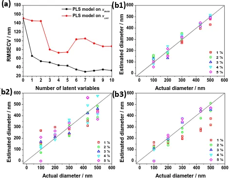
15 From Table 2 it is seen that using the MSC parameters to estimate dˆ leads to an appreciable p
327
reduction in the estimation errors. Using PLS models built on either xmeas or xcorr leads to similar
328
performance in terms of RMSECV which is also evident in the RMSECV curves for the two models in 329
Fig. 8(a). All the three equations used to predict dˆ using MSC parameters (Eqs. (5), (6), and (8)) lead p
330
to appreciable reduction in the error compared to the PLS models. Eqs. (5) and (6) which use MSC 331
parameters a and b respectively give more or less similar performance with around 55% reduction in 332
error. Eq. (8) which combines the information contained in a and b provides the best performance with 333
around 70% reduction in error. The predicted versus the actual diameters for the two PLS models and 334
the model using Eq. (8) are given in the Supporting Information (Figxx). As mentioned previously the 335
use of Eqs. (5), (6), and (8) for obtaining dˆ requires the concentration of the particles to be estimated, p
336
and this was provided using PLS model built on the spectra for this purpose. Table 2 summarizes the 337
performance of PLS models built on un-corrected xmeas and the scatter-corrected xcorr spectra to predict
338
particle concentration. As expected the estimation error in concentration is lower when xcorr are used. If
339
the scatter correction method is effective in selectively removing the underlying scattering and other 340
non-chemical effect, then it should lead to a better PLS model for predicting particle concentration. . 341
Therefore when using the three equations (Eqs. (5), (6) and (8)), the concentrations of particles 342
estimated from the corrected spectra were provided as input. 343
3.2.2 Four-component system
344
In the case of 4-component system, the results were different from that observed in the 2-component 345
dataset. From Table2, the lowest error in predicting particle diameter is obtained using a PLS model 346
built on the spectra without scatter correction (xmeas). The PLS model built on xcorr leads to more than
347
100% increase in the error. .. The best model for predicting the particle diameter using the MSC 348
parameters was given by Eq. (11) which combines information in a, b, and xcorr. Unlike the
2-349
16 xmeas. The reason for this was investigated first by examining the performance of the PLS model to
351
predict particle concentration which is an input for Eq. (11). From Table 2, it is seen that RMSECV for 352
the estimated concentration is much higher compared to the 2-component dataset. Both xmeas and xcorr
353
give similar levels of error in the estimated concentration though the model built onxcorr requires fewer
354
numbers of latent variables. If the large error in estimated diameter dˆp is due to the error contributed
355
by yˆ, then by replacing yˆ by the actual concentration y should result in significant improvement and
356
lead to similar performances that seen for the 2-component dataset. However, the error in estimated dˆp
357
did not reduce significantly indicating that the source of this increase in error lies elsewhere. 358
Further investigation was carried out by examining the concentrations of the different components and 359
their correlation structure. The 4-component dataset was designed to eliminate the concentration 360
correlation between the polystyrene particles and other components of the system. However, in the 361
dataset the particle diameter is weakly correlated to the main constituents of the medium, H2O and D2O
362
with a correlation coefficient of about 0.26 with each of these components. This raises the possibility 363
that the PLS model built on xmeas for estimating particle diameter will be improved by such a
364
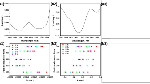
correlation. Examining the scores of the PLS model, it was found that the scores of the first latent 365
variable and to a certain extent the second latent variable are linearly related todp, as indicated in Figs. 366
12(b1) and (b2). Examining the loadings of these two latent variables shown in Figs. 12(a1) and (a2), 367
we see that they appear to be explaining variations that affect the baseline of the spectra i.e. light 368
scattering. Applying MSC and then building a PLS model on xcorr would result in the removal of
369
information regarding particle diameter and should lead to models with higher errors in the estimation 370
of particle size. The scores of the first and second latent variables obtained by applying PLS to xcorr in
371
Figs. 13(b1) and (b2) shows that the first latent variable no longer possesses a clear relationship with 372
particle diameter. Also the first latent variable now resembles more like the second LV for the un-373
17 It is also interesting to note that the number of latent variables required for the PLS model to predict 375
particle diameter is reduced from 7 when xmeas is used to 4 when xcorr is used. This explains the increase
376
in the error in the estimated particle diameter when PLS is applied after scatter correction. Despite this 377
removal of particle size information, the model obtained from xcorr is still statistically significant and
378
almost of similar level of performance as the models using the scatter correction parameters to estimate 379
particle size. This is probably due to the fact that xcorr still has chemical information regarding H2O and
380
D2O which are in turn correlated to the particle diameter thus providing the ability to predict particle
381
diameter despite most of the information regarding this parameter has been removed by scatter 382
correction. The MSC parameters on the other hand, do not include the correlation between particle size 383
and the concentrations of H2O and D2O, since these parameters are indicative of baseline and slope
384
changes in the spectra while absorptivity changes (and thus information) due to concentration changes 385
in H2O and D2O remain in the corrected spectra.
386
Recalling that the MSC parameters for the 4-component dataset are affected by particle size, 387
concentration and the refractive index of the suspending medium (§3.1), it should be pointed out that the 388
models relating particle diameter to the MSC parameters were developed by neglecting the effect of the 389
refractive index changes. This could also potentially lead to an increase in the error in estimating 390
particle diameter. A further point to be noted is that for the 4-component system, the prediction of 391
particle size by using equations that arise from inverting the expressions relating a or b (i.e. Eqs. 9) and 392
(10)) led to two positive values for the particle diameter when the quadratic equations are solved. The 393
ambiguity resulting from this meant that the expressions were not practically usable and therefore the 394
results pertaining to these inverted equations are not shown in Table 1. This problem was not 395
encountered when the combined Eq. (11) was used. Since the equations relating the MSC parameters to 396
particle diameter and concentration that are given here are not necessarily unique, it may be possible to 397
develop an alternative regression model to overcome this problem. 398
18 This study provides an insight into the nature of information contained in the scatter correction 400
parameters. It shows that a scatter correction technique which leads to better calibration models for 401
estimating concentration of chemical species need not necessarily be the best in terms of the scatter 402
correction parameters containing extractable information. It was found that the MSC parameters 403
contained significant information regarding scatter-causing properties namely particle size and 404
concentration. The parameters from EMSC which leads to better performing calibration models 405
compared to MSC do not show a clear relationship with the scatter-causing properties. This may be due 406
to the fact that the information is spread over a larger number of parameters and also the possibility that 407
EMSC might be removing other non-chemical variations that may be presented in the dataset. Further, 408
whether a clear relationship between the MSC parameters and the particle size and concentration was 409
observed depended strongly on the measurement configuration, indicating that the performance of a 410
scatter correction technique will depend on the measurement configuration. This is in line with the 411
observations made in an earlier study based on simulations.[8] 412
Given that the information regarding particle size is present in the MSC parameters, a method to 413
extract this information was proposed and evaluated using the two-component and four-component 414
datasets. It was found that for the 2-component dataset, the method was effective in extracting this 415
information and the model resulting from this method led to a reduction of about 70% in the error in the 416
estimation of particle size compared to models obtained by applying PLS to the spectra. For the 4-417
component dataset, the error in using the proposed method was considerably higher. This appears to be 418
due to the increased uncertainty contributed by the changes in the refractive index of the suspending 419
medium which is not included in the model. Also the PLS model built on the spectra led to considerably 420
lower error compared to the proposed method. Analysis indicates that this is due to chance correlations 421
between particle diameter and the concentrations of D2O and H2O present in the mixture.
422
423
19 [1] A. Rinnan, F.v.d. Berg, S.B. Engelsen, Trends Anal. Chem. 28 (2009) 1201.
425
[2] P. Geladi, D. MacDougall, H. Martens, Appl. Spectrosc. 39 (1985) 491. 426
[3] R.J. Barnes, M.S. Dhanoa, S.J. Lister, Appl. Spectrosc. 43 (1989) 772. 427
[4] S. Wold, H. Antti, F. Lindgren, J. Öhman, Chemom. Intell. Lab. Sys. 44 (1998) 175. 428
[5] H. Martens, J.P. Nielsen, S.B. Engelsen, Anal. Chem. 75 (2003) 394. 429
[6] Z.-P. Chen, J. Morris, E. Martin, Anal. Chem. 78 (2006) 7674. 430
[7] K. Wang, G. Chi, R. Lau, T. Chen, Anal. Lett. 44 (2011) 824. 431
[8] S.N. Thennadil, E.B. Martin, J. Chemom. 19 (2005) 77. 432
[9] R. Steponavicius, S.N. Thennadil, Anal. Chem. 81 (2009) 7713. 433
[10] R. Steponavicius, S.N. Thennadil, Anal. Chem. 83 (2011) 1931. 434
[11] S.N. Thennadil, H. Martens, A. Kohler, Appl. Spectrosc. 60 (2006) 315. 435
[12] C.F. Bohren, D.R. Huffman, Absorption and Scattering of Light by Small Particles, Wiley-VCH, 436
Berlin, 2004. 437
[13] A. Engdahl, B. Nelander, J. Appl. Phys. 86 (1987) 1819. 438
[14] J.P. Devlin, J. Appl. Phys. 112 (2000) 5527. 439
[15] M.M. Reis, P.H.H. Araújo, C. Sayer, R. Giudici, Macromol. Rapid Commun. 24 (2003) 620. 440
[16] K. Ito, T. Kato, T. Ona, J. Raman Spectrosc. 33 (2002) 466. 441
[17] A. Gupta, G.E. Peck, R.W. Miller, K.R. Morris, J. Pharm. Sci. 93 (2004) 1047. 442
[18] J. Rantanen, H.k. Wikström, R. Turner, L.S. Taylor, Anal. Chem. 77 (2004) 556. 443
Stage 1 Stage 2
Apply PLS model to predict Scatter correction
method
Estimate (Eqs. (A.6), (A.7) or (A.8))
Spectra of unknown
samples (xmeas)
xmeas
xcorr
ˆ y
[a, b]
Estimate coeff. in Eqs. (A.4) and (A.5)
ˆ
p d
Build PLS model to predict y Calibration set of different dp and y
Measurement on the samples (xmeas)
Scatter correction method
Substitute coeff. into inverse relation
ˆ y
xmeas
xcorr
[a, b]
y
xref
y dp
coeff.
Obtain and yˆ dˆp
Figure 1
Figure 2
1550 1600 1650 1700 1750 1800 1850 0.2
0.4 0.6 0.8 1.0 1.2 1.4 1.6 1.8
-lo
g
xmea
s
Wavelength / nm
1550 1600 1650 1700 1750 1800 1850 0.4
0.5 0.6 0.7 0.8 0.9
-lo
g
xcorr
Wavelength / nm
(a) (b)
Fig. 3. (a) Changes in MSC parameter a in the 2-component system with (a1) particle diameter and (a2) concentrations. (b) Changes in MSC b with (b1) particle diameter and (b2)
concentrations. Solid curves were generated from the best fit obtained using least squares regression.
Figure 3
100 200 300 400 500 -0.1
0.0 0.1 0.2 0.3
a
Particle diameter / nm 0.1 %
0.5 % 0.9 % 1.23% 1.6 % 1.95% 2.3 %
0.0 0.5 1.0 1.5 2.0 2.5 -0.2
-0.1 0.0 0.1 0.2 0.3 0.4
a
Particle concentration / % 100 nm
200 nm 300 nm 430 nm 500 nm
(a1)
(a2)
100 200 300 400 500 0.8
0.9 1.0 1.1 1.2 1.3 1.4 1.5 1.6
b
Particle diameter / nm 0.1 %
0.5 % 0.9 % 1.23% 1.6 % 1.95% 2.3 %
0.0 0.5 1.0 1.5 2.0 2.5 0.8
0.9 1.0 1.1 1.2 1.3 1.4 1.5 1.6
b
Particle concentration / % 100 nm
200 nm 300 nm 430 nm 500 nm
(b1)
Figure 4
1500 1550 1600 1650 1700 1750 1800 1850 0.4
0.6 0.8 1.0 1.2 1.4
-lo
g
xmea
s
Wavelength / nm
1500 1550 1600 1650 1700 1750 1800 1850 0.8
0.9 1.0 1.1 1.2
-lo
g
xcorr
Wavelength / nm
(a) (b)
Figure 5
1 2 3 4 5
0.2 0.4 0.6 0.8 1.0 1.2 1.4 1.6 1.8 2.0
100 nm 200 nm 300 nm 430 nm 500 nm
b
Particle concentration / %
1 2 3 4 5
-0.5 0.0 0.5 1.0 1.5
a
Particle concentration / %
100 nm 200 nm 300 nm 430 nm 500 nm
100 200 300 400 500 0.2
0.4 0.6 0.8 1.0 1.2 1.4 1.6
b
Particle diameter / nm
1 % 2 % 3 % 4 % 5 %
100 200 300 400 500 -0.8
-0.6 -0.4 -0.2 0.0 0.2 0.4 0.6 0.8 1.0
a
Particle diameter / nm
1% 2% 3% 4% 5%
(a1)
(a2)
(b1)
(b2)
Fig. 6. (a) Simulated total reflectance spectra (Rd_sim) of the 4-component dataset. (b) MSC preprocessed spectra (Rd_simcorr) using the mean of Rd_sim as a reference spectrum. The bulk absorption and scattering coefficients used for the simulation are in (c) and (d), respectively.
Figure 6
1500 1550 1600 1650 1700 1750 1800 1850 0.4
0.6 0.8 1.0 1.2 1.4
-log
R
d_sim
Wavelength / nm
1500 1550 1600 1650 1700 1750 1800 1850 0.8
0.9 1.0 1.1 1.2
-lo
g
Rd_s
im
co
rr
Wavelength / nm
(a) (b)
1500 1550 1600 1650 1700 1750 1800 1850 0.0
0.5 1.0 1.5 2.0 2.5
a
Wavelength / nm
Figure 7
Fig. 7. Results of simulated spectra (Rd_sim) of the 4-component system after MSC preprocessing. (a) Changes in MSC parameters a with (a1) particle diameter and (a2) concentrations. (b) Changes in MSC b with (b1) particle diameter and (b2)
concentration. Solid curves were generated from the best fit obtained by least squares regression.
1 2 3 4 5
0.2 0.4 0.6 0.8 1.0 1.2 1.4 1.6 1.8 2.0
100 nm 200 nm 300 nm 430 nm 500 nm
b
Particle concentration / %
100 200 300 400 500 -0.8
-0.6 -0.4 -0.2 0.0 0.2 0.4 0.6 0.8 1.0
a
Particle diameter / nm 1%
2% 3% 4% 5%
1 2 3 4 5
-0.5 0.0 0.5 1.0 1.5
100 nm 200 nm 300 nm 430 nm 500 nm
a
Particle concentration / %
(a1)
(a2)
(b1)
Figure 8
0 100 200 300 400 500 600 0
100 200 300 400 500 600
0.1% 0.5% 0.9% 1.23% 1.6% 1.95% 2.3%
Estim
at
ed di
ameter
/
nm
Actual diameter / nm
0 100 200 300 400 500 600 0
100 200 300 400 500 600
0.1% 0.5% 0.9% 1.23% 1.6% 1.95% 2.3%
Estim
at
ed di
ameter
/
nm
Actual diameter / nm 0 1 2 3 4 5 6 7 8 9 10 60
80 100 120 140 160
R
MS
EC
V
/
nm
Number of latent variables PLS model on x
meas
PLS model on x corr
0 100 200 300 400 500 600 0
100 200 300 400 500 600
0.1% 0.5% 0.9% 1.23% 1.6% 1.95% 2.3%
Estim
at
ed di
ameter
/
nm
Actual diameter / nm
(a)
(b2)
(b1)
(b3)
Figure 9
0.0 0.5 1.0 1.5 2.0 2.5
0.0 0.5 1.0 1.5 2.0 2.5
100 nm 200 nm 300 nm 430 nm 500 nm
Estimated Conce
ntration / %
Actual concentration / %
0.0 0.5 1.0 1.5 2.0 2.5
0.0 0.5 1.0 1.5 2.0 2.5
100 nm 200 nm 300 nm 430 nm 500 nm
Estimated Conce
ntration / %
Actual concentration / %
1 2 3 4 5 6 7 8 9 10
0.0 0.1 0.2 0.3 0.4 0.5 0.6 0.7
RMSE
CV /
%
Number of latent variables
PLS model on xmeas
PLS model on xcorr
(a) (b1) (b2)
Figure 10
0 100 200 300 400 500 600 0 100 200 300 400 500 600 1 % 2 % 3 % 4 % 5 % Estim at ed di ameter / nm
Actual diameter / nm
0 1 2 3 4 5 6 7 8 9 10
20 40 60 80 100 120 140 160 180 R MS EC V / nm
Number of latent variables PLS model on xmeas
PLS model on xcorr
0 100 200 300 400 500 600 0 100 200 300 400 500 600 1 % 2 % 3 % 4 % 5 % Estim at ed di ameter / nm
Actual diameter / nm
0 100 200 300 400 500 600 0 100 200 300 400 500 600 1 % 2 % 3 % 4 % 5 % Estim at ed di ameter / nm
Actual diameter / nm
(a)
(b2)
(b1)
(b3)
Fig. 10. (a) RMSECV curves of PLS models for estimating particle diameter in 4-component system. (b1) and (b2) are the prediction using PLS models built on xmeas and
Figure 11
0 1 2 3 4 5 6 7 8 9 10
0.4 0.6 0.8 1.0 1.2 1.4 1.6 1.8
R
M
S
E
C
V
/
%
Number of latent variables
PLS model on xmeas
PLS model on xcorr
0 1 2 3 4 5 6
0 1 2 3 4 5 6
100 nm 200 nm 300 nm 430 nm 500 nm
Esti
mated
C
o
n
cen
tr
ati
o
n
/
%
Actual concentration / %
0 1 2 3 4 5 6
0 1 2 3 4 5
6 100 nm
200 nm 300 nm 430 nm 500 nm
Esti
mated
co
n
cen
tr
ati
o
n
/
%
Actual concentration / %
(a) (b1) (b2)
1500 1550 1600 1650 1700 1750 1800 1850 -0.1 0.0 0.1 0.2 0.3 0.4 Loa din g 2
Wavelength / nm
1500 1550 1600 1650 1700 1750 1800 1850 0.068 0.070 0.072 0.074 0.076 0.078 0.080 0.082 0.084 0.086 Loa din g 1
Wavelength / nm
6 8 10 12 14 16 18 20
100 200 300 400 500 1 % 2 % 3 % 4 % 5 % Pa rtic le di a me ter / nm Score 1
-0.4 -0.2 0.0 0.2 0.4
100 200 300 400 500 Pa rtic le di a me ter / nm Score 2
-0.4 -0.2 0.0 0.2 0.4
100 200 300 400 500 Pa rtic le di a me ter / nm Score 3
1500 1550 1600 1650 1700 1750 1800 1850 -0.10 -0.05 0.00 0.05 0.10 0.15 0.20 Loa din g 3
Wavelength / nm
(a1) (a2) (a3)
(b1) (b2) (b3)
Figure 12
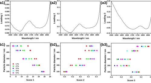
[image:31.540.21.520.96.370.2]Figure 13
Fig. 13. (a1)-(a3) loading curves and (b1)-(b3) scores of the first 3 loadings of the PLS model built on xcorr to estimate particle diameter.
12.8030 12.8035 12.8040 12.8045 12.8050 12.8055 100
200 300 400
500 1 %
2 % 3 % 4 % 5 %
Pa
rtic
le
di
a
me
ter
/
nm
Score 1
-0.4 -0.2 0.0 0.2 0.4
100 200 300 400 500 1 % 2 %
3 % 4 % 5 %
Pa
rtic
le
di
a
me
ter
/
nm
Score 2
1500 1550 1600 1650 1700 1750 1800 1850 0.065
0.070 0.075 0.080 0.085 0.090
Loa
din
g 1
Wavelength / nm
1500 1550 1600 1650 1700 1750 1800 1850 -0.15
-0.10 -0.05 0.00 0.05 0.10
Loa
din
g 2
Wavelength / nm
(a1) (a2)
(b1) (b2)
(a3)
[image:32.540.17.507.71.348.2]