Predictive PDF Control in Shaping of Molecular Weight
Distribution Based on a New Modeling Algorithm
Jinfang Zhanga, Hong Yueb,∗, Jinglin Zhouc
aSchool of Control and Computer Engineering, North China Electric Power University,
Beijing, 102206, P.R. China
bDepartment of Electronic and Electrical Engineering, University of Strathclyde,
Glasgow, G1 1XW, UK
cCollege of Information Science and Technology, Beijing University of Chemical
Technology, Beijing, 100029, P.R. China
Abstract
The aims of this work are to develop an efficient modeling method for es-tablishing dynamic output probability density function (PDF) models using measurement data and to investigate predictive control strategies for con-trolling the full shape of output PDF rather than the key moments. Using the rational square-root (RSR) B-spline approximation, a new modeling al-gorithm is proposed in which the actual weights are used instead of the pseudo weights in the weights dynamic model. This replacement can reduce computational load effectively in data-based modeling of a high-dimensional output PDF model. The use of the actual weights in modeling and control has been verified by stability analysis. A predictive PDF model is then con-structed based on which predictive control algorithms are established with the purpose to drive the output PDF towards the desired target PDF over the control process. An analytical solution is obtained for the non-constrained predictive PDF control. For the constrained predictive control, the optimal solution is achieved via solving a constrained nonlinear optimization problem. The integrated method of data-based modeling and predictive PDF control is applied to closed-loop control of molecular weight distribution (MWD) in an exemplar styrene polymerization process, through which the modeling ef-ficiency and the merits of predictive control over standard PDF control are
∗Corresponding author. Tel. +44 141 5482098
demonstrated and discussed.
Keywords: Probability density function (PDF), B-spline approximation, parameter estimation, model predictive control (MPC), molecular weight distribution (MWD)
1. Introduction
Polymers are materials composed of macromolecules with different chain lengths, and the macromolecular architectures govern the properties of poly-mers such as thermal properties, stress−strain properties, impact resistance, strength, and hardness that affect end-use applications [1, 2]. The molecular weight distribution (MWD) is a major index featuring molecular and compo-sitional characteristics of a polymer, therefore is one of the most important variables to be controlled in industrial polymerization processes. Compared with most control systems that aim to drive the output variables to follow desired set points in time domain, the shaping of MWD is much more com-plicated in modeling and controller design since the term to be controlled is a distribution function that needs to follow a target distribution. The lack of on-line measurement of MWD is another main problem in closed-loop control of polymerization reactions. Sensors like infrared and Raman scat-tering, mainly measure monomer conversion, not polymer molecular weight. Soft measurement of MWD through mathematical modeling is still the pri-mary means to provide online information on MWD for control purposes. Mathematical models of MWD developed based on reaction mechanisms are normally nonlinear and of high dimensions. In the past decades, a number of methods have been developed for MWD control in polymerization processes [3, 4, 5, 6, 7, 8, 9, 10, 11]. An earlier review on modeling and optimization of particulate polymerization processes is given in [12].
in furnace systems [24, 25], power PDF control in nuclear research reactors [26], and bubble size distribution control in flotation processes [27], to name a few. To tackle the control problems for such systems, the idea of output stochastic distribution control (SDC) or output PDF control has been pro-posed, in which the full shape of the output distribution is directly controlled [28, 29, 30, 31, 32]. Unlike mean-and-variance control and other moment-based control, output PDF control can be applied to systems with output function of arbitrary distribution shape and subject to non-Gaussian noise terms. The purpose of output PDF control is to drive the output PDF to-wards the desired target PDF over the control process. It is fundamentally difficult to control the output distribution with a limited number of control inputs. In this work, we hope to make progress to tackle this challenging task from both modeling and control point of view.
Developing a general dynamic model to describe output PDF as a func-tion of control input is the first step towards closed-loop control. Developing a reliable output PDF model from measurement data of control input and output distribution for any practical systems is a very challenging task. B-spline models are often used in output PDF approximation. The major ad-vantage of a B-spline PDF model is the decoupling of time domain and PDF definition domain in formulation. Several B-spline based PDF models are developed, among them the simplest one is the linear B-spline PDF model, where the output PDF is approximated by B-spline basis functions linearly combined together, that is , γ(y, u) = Pn
i=1ωi(u)Bi(y), where γ(y, u) is the
output PDF defined in a bounded region [a, b]; y ∈ [a, b] is an independent variable in the probability distribution space (note y is not used to describe the system output as normally appeared in control literature). u is the con-trol input. Bi(y)(i = 1· · ·n) are the B-spline basis functions defined in a
specific range. ωi(u) is the weight associated with Bi(y). n is the number
of basis functions used, increasing which will improve approximation accu-racy but cost more computational efforts. Considering the example of MWD modeling in a polymerization process, y can be used to stand for the chain length,uis the manipulated variable such as the ratio of monomer and cata-lyst flows,γ(y, u) is the MWD to be controlled. Linear B-spline models have been used in our earlier studies of MWD modeling and closed-loop control system design [8, 33].
integration constraint of R γ(y, u)dy = 1 must always apply for any PDFs in its definition domain. To cope with this integration constraint, a rational B-spline model is proposed [35]. Combining the square-root model and the rational spline model together, the so-called rational square-root (RSR) B-spline model is developed [36], which guarantees both the non-negativeness nature of a PDF and the integration constraint.
p
γ(y, u) =
Pn
i=1ωi(u)Bi(y)
q
Pn
i,j=1ωiωj
Rb
aBi(y)Bj(y)dy
(1)
In this work, the RSR B-spline PDF model is further investigated so as to improve the computational efficiency in the data-based modeling procedure. It is one of our major aims to develop an efficient modeling algorithm for establishing dynamic output PDF models using data of control input and output PDF. This is significantly different from most existing works in output PDF control that were developed based on assumed models.
MWD control [42]. In this work, it is aimed to develop a predictive control scheme to control the full shape of MWD by considering control constraints. The rest of this paper is organized as follows. In Section 2, a new mod-eling algorithm is proposed which employs the rational square-root (RSR) B-spline model for output PDF approximation. The rationale of using the actual weights instead of the pseudo weights is discussed with a strict stabil-ity analysis. A predictive PDF model is established in Section 3, based on which two predictive PDF control strategies are developed in Section 4. Sim-ulation study of an exemplar MWD control system in styrene polymerization is carried out in Section 5 to evaluate the modeling efficiency and the control performances under different strategies. Conclusions are given in Section 6.
2. Data-based model development using RSR B-spline PDF ap-proximation
2.1. RSR B-spline model for output PDF approximation
An output PDF control system is normally a nonlinear dynamic system, for which a nonlinear dynamic weights model is expected. However, due to the distribution characteristic in output, development of a nonlinear output PDF model using input data and output PDF data is extremely difficult. A reasonable assumption can be made that near the operating point, there is no essential difference between the linear weights dynamic models in [17] and the nonlinear weights models in [32] with Lipschitz assumptions. In this work, linear dynamics in weights are considered and the discrete-time RSR B-spline PDF model can be represented as follows:
V(k+ 1) =AV(k) +Bu(k) (2)
p
γ(y, k) = pC(y)V(k)
VT(k)EV(k) (3)
where
C(y) = [B1(y), B2(y),· · · , Bn(y)] (4)
E =
Z b
a
CT(y)C(y)dy (5)
matrix E is invertible. Here V(k) = [ω1(k), ω2(k),· · · , ωn(k)]T is called the
pseudo weights vector in the RSR B-spline model since it cannot be uniquely determined from γ(y, k). The actual weights vector is defined as [36]
Vr(k) =
V(k)
p
VT(k)EV(k). (6)
It is apparent that Vr(k)TEVr(k) = 1 for all k.
To establish a complete dynamic model as in (2)-(3) using the data of control input and output PDF, one needs to calculate V(k) to obtain the PDF approximation weights at each time k, and estimate all parameters in
A andB to establish the weights dynamics. It can be seen from (3) that the pseudo weightsvector is difficult to be determined since the model regarding
V(k) is nonlinear and also V(k) is not unique, however, the actual weights vector, Vr(k), can be uniquely calculated from the PDF function γ(y, k) as
explained in the following.
Left multiplying CT(y) to both sides of (3) and then taking integration for y on both sides leads to
Z b
a
CT(y)
q
γ(y, k)dy=
Z b
a
CT(y)C(y)dyVr(k) = EVr(k) (7)
As discussed earlier E is invertible, therefore the actual weights vector can be calculated from the output PDF by
Vr(k) =E−1
Z b
a
CT(y)pγ(y, k)dy (8)
While it is impossible to uniquely determine the pseudo weights, V(k), from an output PDF, a straightforward solution to calculate the B-spline actual weights, Vr(k), is provided in (8). The rationale of using Vr(k) in
replacing V(k) is further discussed in the next section. 2.2. Feasibility analysis on the use of actual weights
Denoting e(k) =V(k)−Vg, where Vg is the vector of the actual weights
corresponding to the desired PDF γg(y), i.e. VgTEVg = 1, the following error
dynamic system can be established for model (2)-(3):
The purpose of controller design is to choose a control sequence u(k) such that the system’s output PDF follows a pre-specified continuous PDF γg(y)
as close as possible. Here γg(y) is also defined on [a, b] and is independent of
u(k). This is equivalent to choosing an augmented controller ¯
u(k) = (BTB)−1BT(A−I)Vg +u(k), (10)
such that pγ(y,u¯(k)) follows pγg(y) as close as possible. As a result, ¯u(k)
can be designed in the form of output feedback control for the error dynamic system (9),
¯
u(k) =K(k), (k) =
Z b
a
p
γ(y,u¯(k))−
q
γg(y)
dy
= Σ0(Vr(k)−Vg) (11)
where Σ0 =RabC(y)dy.
The following Lemma is presented for stability analysis of controller (11) in which the actual weights vector is used.
Lemma 1. For a function f(α, β) = √αTEα−pβTEβ, E > 0, there is a
ρ with kρk ≤ √λmax(E)
λmin(E)
such that
kf(α, β)k ≤ρkkαk − kβkk
where k · k is Euclidean norm. λmax(E) and λmin(E) are the absolute maxi-mum and minimaxi-mum eigenvalue of E, respectively.
Proof.
kf(α, β)k=
αTEα−βTEβ
√
αTEα+pβTEβ
≤ kEk
(α−β)T(α+β)
√
αTEα+pβTEβ
≤ λmax(E)
(α−β)T(α+β)
p
λmin(E)
√
αTα+pβTβ
The feedback controller (11) is formulated on the actual weights and has the following stability Theorem.
Theorem 1. Selecting
K =LqVT
g EVg (12)
if there is an L so that A+BLΣT
0 is Hurwitz, then the asymptotical stability of the error dynamic system (9) can be guaranteed by feedback control (11).
Proof. Substituting (12) into (11), we have
(k) = qΣ0e(k)
VT
g EVg
+Σq0V(k)Λ1
VT
g EVg
,
where Λ1 =
q VT
g EVg
VT(k)EV(k) −1, and the error dynamic can be written as
e(k+ 1) =Ae(k) +BL
q
VT
g EVg(k)
= (A+BLΣ0)e(k) +BLΣ0V(k)Λ1. Since G = A +BLΣT
0 is Hurwitz, there exists a unique positive definite symmetrical matrix P that satisfies the following Lyapunov equation
GTP G−P =−I. (13)
Choose the following Lyapunov function
π(e(k)) = eT(k)P e(k), (14)
then
∆π = π(e(k+ 1))−π(e(k))
= − ke(k)k2+ 2eT(k)GTP BLΣ0V(k)Λ1 + (BLΣ0V(k)Λ1)TP (BLΣ0V(k)Λ1)
≤ − ke(k)k2+ 2
GTP BLΣ0
λke(k)k
2
p
λmin(E)
+kP BLΣ0k 2
λ2ke(k)k2
λmin(E)
Moreover, if
kLk ≤ (−µ1+
p
µ2 1+ 4ν)
p
λmin(E)
2ν
where µ1 =
GTP BΣ0
ρ and ν =kP BΣ0k
2
ρ2, then ∆π ≤0, which means this feedback control system is asymptotically stable.
From Theorem 1, it is known that if matrix G is Hurwitz, there exists an output feedback controller that is based on the actual weights. Therefore, when V(k) in the controller is replaced by the actual weights, this controller can be taken as a special output feedback controller. In other words, when an output PDF model satisfies the condition thatGbeing stable, at each control interval, the actual weights can be used to replace the pseudo weights. This supports our idea of using the actual weights to construct the RSR B-spline PDF model for controller design.
2.3. Parameterization algorithm for data-based PDF modeling
Using theactual weights, the following output PDF system is proposed.
Vr(k+ 1) = ¯AVr(k) + ¯Bu(k) (15)
p
γ(y, k) =C(y)Vr(k) (16)
¯
A and ¯B are matrices of the same dimensions as A and B in (2). For the same input, this model can be regarded as ’practically equivalent’ to model (2)-(3), i.e., in the transient process, the output error between these two models are within an acceptable small range, and in the steady state, their output values are the same. The use of ’practically equivalent model’ or ’characteristic model’ in real engineering control systems was proposed and discussed in [43]. In the rest of the paper, the new RSR B-spline model in (15)-(16) will be used in parameter estimation and controller design.
Denote
f(y, k) = pγ(y, k) (17)
as a function representing the output PDF at each time k. From (15)-(16), the function of output PDF can be written as
f(y, k) = C(y)Vr(k)
Expanding (18) brings the parameterized model
f(y, k) = a1f(y, k−1) +· · ·+anf(y, k−n)
+C(y)D0u(k−1) +C(y)D1u(k−2) +· · ·
+C(y)Dn−1u(k−n) (19) Note each Di(i = 0,· · · , n − 1) is an n-dimensional vector which can be
written as Di = [di1, di2, . . . , din]T.
Let
ψ(y, k) = [f(y, k−1),· · · , f(y, k−n),
u(k−1)B1(y),· · · , u(k−1)Bn(y),· · · ,
u(k−n)B1(y),· · · , u(k−n)Bn(y)]T,
and write the vector of parameters as
θ = [a1,· · · , an, d01,· · · , d0n, d11,· · · ,
d1n,· · · , d(n−1)1,· · · , d(n−1)n]T,
equation (19) can be rewritten into a compact form as
f(y, k) =θTψ(y, k). (20)
Whennbasis functions are used in the PDF approximation, the total number of parameters to be estimated in θ is n×(n+ 1). This suggests that model (20) is normally of high dimension in an output PDF control system.
Given the B-spline basis functions, least-square algorithms can be applied to recover the parameters in θ when the data of control input and output PDF is collected. Due to the large number of parameters included in the modeling, the following double-loop recursive least-square (RLS) algorithm is used to estimate θ by screening the PDF definition domain of [a, b] for y
(inner loop, indexed by i) and going through the time domain for k (outer loop):
ˆ
θ(i, k) = ˆθ(i−1, k) + P(i−1, k)ψ(y(i), k)ε(i, k)
1 +ψT(y(i), k)P(i−1, k)ψ(y(i), k) (21)
ε(i, k) =f(y(i), k)−θT(i−1, k)ψ(y(i), k) (22)
P(i, k) =
I− P(i−1, k)ψ(y(i), k)ψ
T(y(i), k) 1 +ψT(y(i), k)P(i−1, k)ψ(y(i), k)
The initial value of the RLS algorithm is set to be ˆθ(0,0) = θ0, P(0,0) = 103−6In(n+1), P(0, k) =P(M, k−1) and ˆθ(0, k) = ˆθ(M, k−1) fork ≥1. M is the total number of samplings in the region of [a, b].
The procedures for establishing the RSR B-spline PDF model can be summarized as follows.
S0: Initialize relevant terms atk = 0. Define data set{y(i)}, i= 1,· · ·, M, in the definition interval [a, b] for y. Set k = 1 for the recursive opera-tion.
S1: At sampling time k, collect the input data u(k) and the output PDF data γ(y(i), k).
S2: Calculate f(y(i), k) following (17).
S3: Estimate θ using the RLS algorithm in (21)-(23) for i= 1· · ·M. S4: Increase k tok+ 1, repeat S1–S3 until the end of the calculation.
The parameterized input-output model (19) can be used for output PDF control in general cases. However, this model is inadequate for predictive PDF control since there is no prediction function provided. In the next sec-tion, a predictive PDF model will be constructed to facilitate the development of predictive PDF control strategies.
3. Construction of predictive PDF model
Equation (19) can be written as
f(y, k) =
n
X
i=1
aif(y, k−i) + n−1
X
j=0
C(y)Dju(k−j−1). (24)
Introducing the back-shift operator z−1, denote
α(z−1) = 1−
n
X
i=1
aiz−i, β(z−1, y) = C(y) n−1
X
j=0
Djz−j, (25)
equation (24) can be represented as
α(z−1)f(y, k) =β(z−1, y)u(k−1). (26)
The following Diophantine equation is introduced to construct the pre-dictive PDF model
where q is the index for model prediction steps, and
Gq(z−1) = 1 + q−1
X
i=1
gq,iz−i, Hq(z−1) = n−1
X
j=0
hq,jz−j. (28)
Multiplying Gq(z−1) to both sides of (26) and taking into account the
Dio-phantine equation (27), we have
f(y, k+q) =Hq(z−1)f(y, k) +Gq(z−1)β(z−1, y)u(k+q−1). (29)
Define
Sq(z−1, y) = Gq(z−1)β(z−1, y) =C(y)
n−1+q−1
X
i=0
sq,iz−i, (30)
and write
¯ C(y) =
C(y) 0 · · · 0
0 C(y) · · · 0
..
. ... · · · ...
0 0 · · · C(y)
.
When taking q = 1,2,· · · , p (p is the model predictive horizon), the multi-step predictive PDF model in (29) can be written into the following matrix format
where
Π(y, k, p) =
f(y, k+ 1)
f(y, k+ 2) .. .
f(y, k+p)
, Hˆ =
H1(z−1)
H2(z−1) .. .
Hp(z−1)
,
Ω(y) =C¯(y)
s1,0 0 · · · 0
s2,1 s2,0 · · · 0 ..
. ... · · · ...
sp,p−1 sp,p−2 · · · sp,p−l
,
Φ(y) =C¯(y)
s1,1 s1,2 · · · s1,n−1
s2,2 s2,3 · · · s2,n−1+1 ..
. ... · · · ...
sp,p sp,p+1 · · · sp,n−1+p−1
,
U(k) =
u(k)
u(k+ 1) .. .
u(k+l−1)
, η(k) =
u(k−1)
u(k−2) .. .
u(k−n+ 1)
.
l (l ≤ p) is the predictive control horizon. Equation (31) gives a compact format of the predictive output PDF model.
The coefficients in the Diophantine equation can be obtained by recursive development [44]. Here only the results are provided (detailed derivation can be found in many literature of standard MPC algorithms). With the initial setting of
calculated as follows for q = 1,· · · , p.
hq,0 =gq+1,q
hq+1,0 =hq,1+gq+1,qα1 =hq,1 +hq,0α1
hq+1,1 =hq,2+gq+1,qα2 =hq,2 +hq,0α2 ..
.
hq+1,n−2 =hq,n−1+gq+1,qαn−1 =hq,n−1+hq,0αn−1
hq+1,n−1 =gq+1,qαn=hq,0αn (33)
Similarly, the coefficients in Sq(z−1, y) can be calculated recursively as
fol-lows.
sq+1,i=sq,i+hq,0Di−q
sq+1,n−1+q =hq,0Dn−1 (34)
where i = 0,1, . . . , n+q−2, and Dm = 0 when m < 0. The initial settings
are s1,i =Di for i= 0,· · · , n−1.
Guidance on the selection of model predictive horizon, p, and control predictive horizon,l, can be found in many MPC literature. In principle, the selection ofpandlneeds to balance several performance requirements such as computational load, dynamic tracking performance, stability and robustness.
4. Predictive PDF controller design
In this section, predictive PDF control algorithms with and without con-trol constraints are developed, respectively, based on the predictive PDF model (31). These MPC algorithms will be compared with a standard PDF controller, the latter is also briefed in the following.
4.1. Standard output PDF control
A general PDF control target is to drive the output PDF to follow the desired distribution. Using the following performance function
J0(u(k)) =
Z b
a
p
γ(y, k)−
q
γg(y)
2
where γg(y) is the target distribution, Q0 is a weighting factor for control input, the optimal control input uat time k is obtained by taking dJdu = 0 to give [17]
u(k) =
Rb
a C(y)D0g(y, k)dy
Rb
a(C(y)D0)
2
dy+Q0
(36)
where
g(y, k) = −
n
X
i=2
aif(y, k−i+ 1)−C(y)Di−1u(k−i+ 1)
+
q
γg(y)−a1f(y, k). (37)
When the input-output model is established, at each timek, the controller design procedures can be summarized as follows.
S1: Formulate g(y, k) as in (37) using the parameterized PDF model (19). S2: Calculate RabC(y)D0g(y, k)dy and
Rb
a (C(y)D0)
2
dy. S3: Obtain the optimal control input u(k) with (36). 4.2. Non-constrained predictive PDF control
The following performance index is formulated in the first predictive PDF control algorithm
J(U(k)) =
Z b
a
[Π(y, k, p)−Γ(y)]T[Π(y, k, p)−Γ(y)]dy
+UT(k)QU(k) (38)
where Γ = [pγg(y),· · · ,
p
γg(y)]T is the target PDF vector,Qis the
weight-ing matrix for control input.
Taking (31) into (38) and denoting
ξ(y, k) = ˆHf(y, k) + Φ(y)η(k) (39) as the known term at time k, the optimization solution to (38) is derived from dJdU = 0 as follows:
U(k) = −
Z b
a
ΩT(y)Ω(y)dy+Q
−1
·
Z b
a
ΩT(y)(ξ(y, k)−Γ(y))dy
.
4.3. Constrained predictive PDF control
Various constraints exist in real control systems such as upper and lower bounds of control input, varying rate in control input and output constraints. Failure in handling control constraints may lead to actuator saturation that will delay required control actions and decrease control performance. Con-strained MPC is therefore widely needed in process control to prevent the manipulated variables from getting saturated or output going out of specific bounds.
Bounded constraints on control input are considered in this section to address actuator saturation or other operational constraints on manipulated variables. To simplify the discussion, constant upper and lower bounds are set for control input as umin ≤ u(k) ≤ umax. Using the same predictive
model as in (31) and the same quadratic performance function as in (38), the constrained MPC for output PDF control can be written as the following optimization problem:
J(U(k)) =
Z b
a
[Π(y, k, p)−Γ(y)]T[Π(y, k, p)−Γ(y)]dy
+UT(k)QU(k)
s.t. Umin U(k)Umax (41)
whereUmax = [umax,· · · , umax]T ∈Rl×1andUmin = [umin,· · · , umin]T ∈Rl×1
are vectors of upper and lower bounds, respectively.
The above predictive controller design with constraints is a nonlinear pro-gramming optimization problem, which do not have an analytical solution in general. Optimization methods like quadratic programming (QP), sequen-tial quadratic programming (SQP), sequensequen-tial unconstrained minimization technique, etc., can be applied to get the optimal solution. It can be seen from (41) and (38) that the two predictive control algorithms have the same optimization performance index, but the way to get the optimal solution is different since the constraints on control input are handled differently in these two algorithms.
5. Simulation study of MWD shaping using predictive PDF control
monomer
reaction tank initiator
Heating oil
MWD modeling PDF
controller c
Polymer product 0
M 0 I
I
F
M
F
F
PDF modeling Predictive
PDF modeling Desired PDF
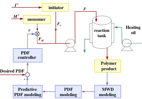
-Figure 1: The sketch of the example polymerization system with predictive PDF control
5.1. Dynamic model of MWD
Consider a styrene polymerization process taking place in a semi-batch continuous stirring tank reactor (CSTR) (Fig. 1). The input flow F to the tank is the sum flow rate of the monomer (FM) and the initiator (FI). The
monomer and the initiator are fed into the reactor with a ratio of C =
FM/(FI+FM), which is used as the control input. The output is the MWD
of the produced polymer. In the simulation, the sum flow rate F is kept constant, only the ratioCbetween the monomer and the initiator is adjusted. The free radical polymerization mechanisms are considered which include initiation, chain propagation, chain transfer to monomer, and termination by combination. Under the framework of population balance, the generation function technique is used to derive the leading moments for MWD model, which are later developed into a parameterized model in the form of a Schultz-Zimm distribution. Full modeling details can be found from the authors’ previous work [8]. The major ordinary differential equations (ODEs) are provided in the following to support the dynamic MWD description.
The concentration equations for initiator, I, and monomer, M, are de-scribed as
dI
dt =
F V (I
0−
I)−KdI (42)
dM
dt =
F
V (M
0−M)−2K
[image:17.612.180.410.129.289.2]tively, in the input flow. Kd is the initiator decomposition rate constant, Ki
is the initiation rate constant,Kp is the propagation rate constant, and Ktrm
is the chain transfer rate constant. ψ0 is the total concentration of radicals. Denote ψk =
P+∞
j=1j
kR
j(k = 0,1,2) as the leading moments for radicals
and Zk =
P+∞
j=2j
kP
j(k = 0,1,2) as the leading moments for dead polymer,
where Rj is the live polymer radical with chain length j and Pj is the dead
polymer with chain length j. The following ODEs are derived using the generation function technique to give
dψ0
dt =−
F
V ψ0+ 2KiI−Ktψ
2
0 (44)
dψ1
dt =−
F
V ψ1+ 2KiI+Kpψ0M −Ktψ0ψ1+KtrmM(ψ0−ψ1) (45) dψ2
dt =−
F
V ψ2+ 2KiI+KpM(2ψ1+ψ0)−Ktψ0ψ2+KtrmM(ψ0−ψ2)
(46) where Kt is the termination rate constant. The ODEs for the leading
mo-ments of polymers, Z0, Z1, Z2, are derived to be
dZ0
dt =−
F
V Z0 +KtrmMoψ0+ Kt
2 ψ 2
0 (47)
dZ1
dt =−
F
V Z1 +KtrmMoψ1+Ktψ0ψ1 (48)
dZ2
dt =−
F
V Z2 +KtrmMoψ2+Ktψ0ψ2+Ktψ
2
1 (49)
Instead of using higher-order moments to describe MWD of styrene polymer-ization product, a Schultz-Zimm distribution is regarded as an appropriate distribution function that can be established from those leading moments of polymer. A normalized Schultz-Zimme distribution function is defined by [45]
f(n) = h
hnh−1exp(−hn/M
n)
Mh
nΓ(h)
, (50)
where n ≥ 0 is the chain length, h is a parameter indicating the distribu-tion breadth, Mn is the number average chain length which is defined as
Mn = Z1/Z0, Γ is the gamma function defined as Γ(h) =
R∞
0 n
h−1e−ndn.
Table 1: MWD model parameters
Parameter Unit Value
Kd min−1 9.48×10¹⁶exp(−30798.5/rT)
Ki L·mol−1·min−1 0.6Kd
Kp L·mol−1·min−1 6.306×10⁸exp(−7067.8/rT)
Ktrm L·mol−1·min−1 1.386×10⁸exp(−12671.1/rT)
Kt L·mol−1·min−1 3.765×10¹⁰exp(−1680/rT)
V L 3.927
F L·min−1 0.0286
T K 353
I0 mol·L−1 0.0106
M0 mol·L−1 4.81
r cal·mol−1·K−1 1.987
C [0.3,0.7]
two parameters of the Schultz-Zimm distribution function can be calculated by the leading moments of polymers as
h = Z
2 1
Z0Z2−Z12
(51)
Mn =Z1/Z0 (52)
In summary, the dynamic MWD modeling includes the following two steps: S1: GetZ0,Z1, Z2 from simultaneous integration of ODEs (42)-(49); S2: Calculate h and Mn from (51) and (52), and formulate MWD by (50).
This first-principle model can be regarded as a soft sensor for MWD measurement, from which the input-output data pairs can be produced for B-spline PDF modeling. Model parameters are listed in Table 1. In this simulation, the chain length of the polymer is from 1 to 2000. The ini-tial conditions for ODEs in (42)-(49) are set up as follows: I(0) = 0.0020,
M(0) = 2.2620, ψ0(0) = 0.0000, ψ1(0) = 0.0000, ψ2(0) = 0.0079, Z0(0) = 0.0014, Z1(0) = 0.6240, Z2(0) = 425.8050. These initial condition values are calculated from static model simulation at a given control ratio C.
0
1000
2000
0 500 1000 15000
1 2 3
x 10−3
chain length
MWD
(a) Data for modeling
0
1000
2000
0 500 1000 15000
1 2 3
x 10−3
chain length
MWD
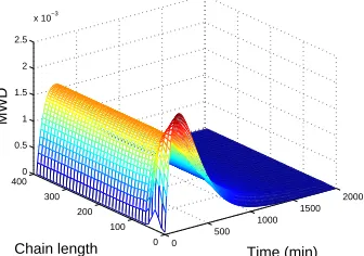
[image:20.612.125.493.137.281.2](b) Model prediction
Figure 2: MWDs from the first-principle model and the B-spline approximation model
as follows:
B(i, j) =
−2/w(i)2 ·(j −y(i)−w(i)/2)2+ 1/2, y(i)≥j ≥y(i) +w(i)
0, otherwise
where j = 1,2,· · · ,2000 stands for the chain length of dead polymers in MWD, and
y(i) = 1 + 200(i−1), i= 1,2,· · ·,10
w(i) =
220, i= 1,2,· · · ,9 199, i= 10
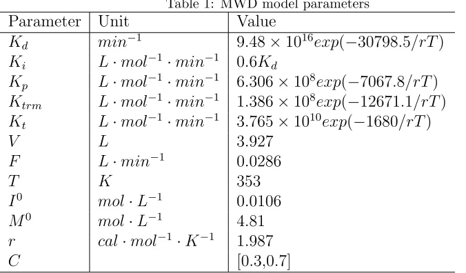
Here i refers to the ith B-spline basis function, w is the parameter for B-spline width. The double-loop RLS algorithm in Section 2.3 is applied to estimate model parameters. Fig. 2(a) shows the 1500 sets of created MWD data used for establishing the RSR B-spline PDF model. Fig. 2(b) illustrates the B-spline modeling result regarding MWDs versus time and chain length. The MWD modeling error, defined by γ1(y, k)−γ2(y, k) between two PDFs, is illustrated in Fig. 3. The scale of Fig. 3 is two-order lower than the MWD modeling data and this shows a good modeling quality.
5.2. Shaping of MWD by predictive output PDF control
0
1000
2000
0 500 1000 1500−4
−2 0 2
x 10−5
chain length
[image:21.612.218.397.136.258.2]MWD
Figure 3: MWD modeling error
distribution is set corresponding to a control level of C = 0.6. In all three control algorithms, the performance indexes for optimization consist of two terms, one for output PDF tracking performance and one for penalty of the control cost weighted by a Q factor. The penalty term needs to be tuned to achieve a balance between a good tracking performance and a low cost of control.
We first apply the standard output PDF control to this system, in which the weighting factor for control input is tuned to beQ0 = 0.0005. We then im-plement the two predictive controllers by setting the model predictive horizon to be p = 9, the control predictive horizon to be l = 5, and Q= 0.0106I5×5 for both controllers. For the constrained MPC, the upper and lower bounds for control input are set to be C ∈ [0.3,0.7]. An SQP algorithm is adopted to solve the constrained nonlinear optimization problem and the f mincon() function is used in Matlab simulation. In the standard control and the non-constrained predictive control, a hard-bound ofC ∈[0.3,0.7] is applied to the control implementation considering the feasible operating conditions for this system, i.e., a ’saturated’C is applied whenever the calculated control input is beyond this boundary domain. In order to compare the MWD tracking performance for each control algorithm, the following performance index
Jt(k) =
Z b
a
p
γ(y, k)−qγg(y)
2
dy
0 50 100 150 200 250 300 350 400 0.3
0.35 0.4 0.45 0.5 0.55 0.6 0.65 0.7 0.75
Time (min)
Ratio C
Standard control Nonconstrained MPC Constrained MPC
(a) Three control actions
0 50 100 150 200 250 300 350 400
0 0.005 0.01 0.015 0.02 0.025 0.03 0.035 0.04 0.045
Time (min)
Tracking performance J
t
Standard control Nonconstrained MPC Constrained MPC
[image:22.612.124.477.130.285.2](b) Three tracking performances
Figure 4: Comparison of control input and tracking performance for 3 controllers (Q0=
0.0005,Q= 0.0106)
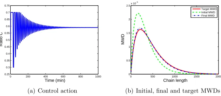
the initial MWD to get closer towards the target MWD over the control pro-cess. The control input profiles for the three controllers are shown in Fig.4(a) and their tracking performances are illustrated in Fig. 4(b). The simulation results show that the non-constrained MPC has the same solution as the con-strained MPC when a hard bound is imposed on the control input (in Fig.4(a) and Fig. 4(b), the curves corresponding to constrained and non-constrained MPCs are completely overlapped). This consistency is not surprising since in both cases the same level of constraints are considered, just handled in dif-ferent manner. Fig. 5 illustrates MWDs at the initial state, the steady state and the desired target state under the standard PDF control and the predic-tive PDF controller, respecpredic-tively. The dynamic evolution of MWDs under the predictive control (constrained and non-constrained) is demonstrated in Fig. 6.
Under the standard output PDF control, it can be seen that there is a clear gap between the MWD at the steady state and the target MWD (Fig. 5(a)), while this steady-state MWD tracking error is much smaller (almost none) with predictive control. In Fig. 5(b), the final MWD curve overlaps with the target PDF curve. The steady-state performance can also be inspected from the control input profiles in Fig. 4(a), where for the two predictive control algorithms the control input signals almost reach the target level ofC = 0.6, when convergent, but the standard control input stays away from the target value at the steady state.
0 500 1000 1500 2000 0
0.5 1 1.5 2
2.5x 10
−3
Chain length
MWD
Target MWD Initial MWD Final MWD
(a) Standard control
0 500 1000 1500 2000
0 0.5 1 1.5 2
2.5x 10
−3
Chain length
MWD
Target MWD Initial MWD Final MWD
[image:23.612.128.479.178.331.2](b) Model predictive control
Figure 5: Initial, final and target MWDs under standard and predictive PDF control
0 500
1000 1500
2000
0 100 200 300 400
0 0.5 1 1.5 2 2.5
x 10−3
Time (min) Chain length
MWD
[image:23.612.223.391.475.593.2]0 200 400 600 800 1000 0.25
0.3 0.35 0.4 0.45 0.5 0.55 0.6 0.65 0.7 0.75
Time (min)
Ratio C
(a) Control action
0 500 1000 1500 2000
0 0.5 1 1.5 2
2.5x 10
−3
Chain length
MWD
Target MWD Initial MWD Final MWD
[image:24.612.126.478.127.281.2](b) Initial, final and target MWDs
Figure 7: Standard output PDF control withQ0= 0.00014
tracking error to the similar level that is achieved by predictive control, then more efforts need to be put on the tracking part of the performance func-tion (35), which means paying a larger price in control to achieve improved tracking performance. To this end, Q0 is reduced from 0.005 to 0.00014, the simulation results of standard control is shown in Fig. 7. It can be seen that in this case, the MWD tracking error at steady state is reduced compared with the results in Fig. 5(a), but the control signal has serious oscillations and it takes a much longer time to reach the steady state.
As discussed in the design of all three output PDF controllers, the output PDF tracking performance is of the major concern, but the cost of control also needs to be considered for practical reasons. Compared with the stan-dard output PDF control, the predictive control algorithms are more capable to achieve a balance between a good tracking performance and a reasonable control action. Also the constraints on control are included in the optimiza-tion process of the constrained predictive PDF control.
6. Conclusion
constraints on positiveness and integration nature for a PDF, which outper-forms three other commonly used B-spline models, i.e., linear, square root and rational B-spline models. With the RSR B-spline model, the actual weights instead of the pseudo weights are used in the data-based modeling of a linear weight dynamic system, which avoids complex estimation of the pseudo weights from output PDF and therefore largely simplifies the model-ing procedure. The parameterized input-output model is further developed into a predictive PDF model that has the function of predicting the full output PDF over a future horizon.
Both non-constrained and constrained predictive control are developed to drive the output PDF towards its target shape. For the non-constrained MPC design, an analytical solution is obtained for a system with linear weight dynamic, which is computationally convenient but may overlook possible sat-uration in control actions. For constrained MPC design, a constrained non-linear optimization problem needs to be solved, which is not a trivial task for a control problem with a full shape expected in its output distribution. The integrated modeling and predictive control scheme is applied to sim-ulation study of an exemplar styrene polymerization process to implement closed-loop MWD control. Simulation results demonstrate the effectiveness of the proposed scheme and show the strength of predictive PDF control over standard output PDF control.
The B-spline based modeling provides a general methodology to describe output PDF control systems which can decouple time domain and space domain (or PDF definition domain) efficiently. The space-varying charac-teristic of the output PDF is approximated by a nonlinear B-spline neural network and the time-varying nature is depicted by a weight dynamic model. Modeling such a system using measurement data is thus a very challenging task since both the static B-spline approximation and the dynamic weights development need to be conducted in the same scheme. In this work, we attempt to explore data-based modeling techniques for output PDF control systems. The ’measurement data’ used in simulation study are produced from a first-principle MWD model that we developed in a previous work. To our knowledge, no other work on data-based modeling of output PDF systems from industrial systems or simulation has been reported.
In addition to B-spline modeling, alternative solutions for output PDF mod-eling could be direct use of output PDF calculated from partial differential equations, estimation of output PDF by unscented Kalman filter, etc.
While MPC shed a light on tackling the output PDF control problem, problems like how to tune the MPC parameters to improve the control per-formance and how to solve the constrained nonlinear optimization effectively need to be further investigated. Since the predictive PDF controller is non-structured and gradient-based, the analysis of closed-loop stability is difficult to perform. Future work on development of structured controllers for output PDF control is under investigation. The fundamental challenge of controlling a full distribution dynamically using a few control inputs remains an open problem for further exploration.
Acknowledgments
This work is partially supported by the Fundamental Research Funds for the Central Universities (2014MS25), NSFC (No. 61374052, No. 61473025), and the open-project grant funded by the State Key Laboratory of Integrated Automation for Process Industry at the Northeastern University, China.
[1] T. J. Crowley, K. Y. Choi, Experimental studies on optimal molec-ular weight distribution control in a batch-free radical polymerization process, Chem. Eng. Sci. 53 (1998) 2769–2790.
[2] T. Takamatsu, S. Shioya, Y. Okada, Molecular weight distribution con-trol in a batch polymerization reactor, Ind. Eng. Chem. Res. 27 (1988) 93–99.
[3] M. F. Ellis, T. W. Taylor, K. F. Jensen, On-line molecular weight distribution estimation and control in batch polymerization, AIChE J. 40 (1994) 445–462.
[4] T. J. Crowley, K. Y. Choi, Discrete optimal control of molecular weight distribution in a batch free radical polymerizaiton process, Ind. Eng. Chem. Res. 36 (1997) 3676–3684.
[6] T. L. Clarke-Pingle, J. F. MacGregor, Optimization of molecular weight distribution using batch-to-batch adjustments, Ind. Eng. Chem. Res. 37 (1998) 3660–3669.
[7] M. Vicente, C. Sayer, J. R. Leiza, G. Arzamendi, E. L. Lima, J. C. Pinto, J. M. Asua, Dynamic optimization of non-linear emulsion copolymer-ization systems open-loop control of composition and molecular weight distribution, Chem. Eng. J. 85 (2002) 339–349.
[8] H. Yue, H. Wang, J. F. Zhang, Shaping of molecular weight distribu-tion by iterative learning probability density funcdistribu-tion control strategies, Proc. IMechE Pt I: J. Syst. Contr. Eng. 222 (2008) 639–653.
[9] H. Y. Wu, L. L. Cao, J. Wang, Gray-box modelling and control of poly-mer molecular weight distribution using orthogonal polynomial neural networks, J. Proc. Control 22 (2012) 1624–1636.
[10] G. Penloglou, E. Kretza, C. Chatzidoukas, S. Parouti, C. Kiparissides, On the control of molecular weight distribution of polyhydroxybutyrate in azohydromonas lata cultures, Biochem. Eng. J. 62 (2012) 39 – 47. [11] S. H. Shen, L. L. Cao, J. Wang, Predictive control of molecular weight
distribution in polymerization reaction based on moment of MWD, CI-ESC J. (in Chinese) 64 (2013) 4379–4384.
[12] C. Kiparissides, Challenges in particulate polymerization reactor mod-eling and optimization: A population balance perspective, J. Proc. Control 16 (2006) 205 – 224.
[13] J. Dimitratos, G. Eliabe, C. Georgakis, Control of emulsion polymer-ization reactors, AIChE J. 40 (1994) 1993 – 2021.
[16] C. D. Immanuel, F. J. D. III, Open-loop control of particle size distribu-tion on semi-batch emulsion copolymerisadistribu-tion using a genetic algorithm, Chem. Eng. Sci. 57 (2002) 4415–4427.
[17] H. Wang, Bounded Dynamic Stochastic Systems: Modelling and Con-trol, Springer-Verlag, London, 2000.
[18] R. A. Eek, O. H. Bosgra, Controllability of particulate processes in relation to the sensor characteristics, Powder Tech. 108 (2000) 137–146. [19] H. J. C. Gommeren, D. A. Heitzmann, J. A. C. Moolenaar, B. Scarlett, Modelling and control of a jet mill plant, Powder Tech. 108 (2000) 147–154.
[20] R. D. Braatz, Advanced control of crystallization processes, Annual Rev. Contr. 26 (2002) 87–99.
[21] E. Aamir, Z. Nagy, C. Rielly, Optimal seed recipe design for crystal size distribution control for batch cooling crystallisation processes, Chem. Eng. Sci. 65 (2010) 3602 – 3614.
[22] Z. K. Nagy, R. D. Braatz, Advances and new directions in crystallization control, Annu. Rev. Chem. Biomol. Eng. 3 (2012) 55–75.
[23] J. S.-I. Kwon, M. Nayhouse, P. D. Christofides, G. Orkoulas, Modeling and control of shape distribution of protein crystal aggregates, Chem. Eng. Sci. 104 (2013) 484 – 497.
[24] X. B. Sun, H. Yue, H. Wang, Modelling and control of the flame tem-perature distribution using probability density function shaping, Trans. Inst. Measurement and Control 28 (2006) 401–428.
[25] J. L. Zhou, H. Yue, J. F. Zhang, H. Wang, Iterative learning dou-ble closed-loop structure for modeling and controller design of output stochastic distribution control systems, IEEE Trans. Control Syst. Tech-nol., In press (2014).
[27] J. Y. Zhu, W. H. Gui, C. H. Yang, H. L. Xu, X. L. Wang, Probability density function of bubble size based reagent dosage predictive control for copper roughing flotation, Contr. Eng. Practice 29 (2014) 1–12. [28] G. A. Smook, Handbook for Pulp and Paper Technologists, Angus Wilde
Publications, Vancouver, 1998.
[29] M. Karny, T. Kroupa, Axiomatization of fully probabilistic design, In-formation Sciences 186 (2012) 105–113.
[30] C. X. Zhu, W. Q. Zhu, , Y. F. Yang, Design of feedback control of a nonlinear stochastic system for targeting a pre-specified stationary probability distribution, Probabilistic Engineering Mechanics 30 (2012) 20–26.
[31] M. Annunziato, A. Borzi, A fokker planck control framework for multi-dimensional stochastic processes, J. Computational and Applied Math-ematics 237 (2013) 487–507.
[32] L. Guo, H. Wang, Stochastic Distribution Control Systems Design: A Convex Optimization Approach, Springer-Verlag, 2010.
[33] H. Yue, J. F. Zhang, H. Wang, L. L. Cao, Shaping of molecular weight distribution using b-spline based predictive probability density function control, in: Proc. 2004 Am. Control Conf., Boston, USA, 2004, pp. 3587–3592.
[34] H. Wang, H. Baki, P. Kabore, Control of bounded dynamic dynamic stochastic distributions using square root models: an applicability study in papermaking system, Trans. Inst. Meas. Control 23 (2001) 51–68. [35] H. Wang, H. Yue, A rational spline model approximation and control
of output probability density functions for dynamic stochastic systems, Trans. Inst. Meas. Contr. 25 (2003) 93–105.
[36] J. L. Zhou, H. Yue, H. Wang, Shaping of output pdf based on the rational square-root b-spline model, Acta Automatica Sinica 31 (2005) 343–351.
[38] R. Findeisen, F. Allgower, An introduction to nonlinear model predictive control, in: 21st Benelux Meeting on Systems and Control, Veldhoven, Netherlands, 2002, pp. 1–23.
[39] E. F. Camacho, C. Bordons, Nonlinear model predictive control: An introductory review, in: R. Findeisen, F. Allgower, L. Biegler (Eds.), Assessment and Future Directions of Nonlinear Model Predictive Con-trol, Springer-Verlag, 2007, pp. 1–16.
[40] B. Alhamad, J. A. Romagnoli, V. G. Gomes, On-line multi-variable predictive control of molar mass and particle size distributions in free-radical emulsion copolymerization, Chem. Eng. Sci. 60 (2005) 6596 – 6606.
[41] T. Kreft, W. F. Reed, Predictive control of average composition and molecular weight distributions in semibatch free radical copolymeriza-tion reaccopolymeriza-tions, Macromolecules 42 (2009) 5558–5565.
[42] J. F. Zhang, H. Yue, J. L. Zhou, A new pdf modelling algorithm and predictive controller design, in: Prepr. 10th IFAC Symp. Dynamics. Contr. Proc. Syst. (DYCOPS2013), Mumbai, India, 2013, pp. 271–276. [43] H. X. Wu, J. Hu, Y. Xie, Characteristic model-based all-coefficient adaptive control method and its applications, IEEE Trans. Syst., Man, Cybern., pt C: Appl. Rev. 37 (2007) 213–221.
[44] D. Q. Shu, Predictive Control and Applications, Mechanical Industry Publishing Company, Beijing, 1996.