Wideband 2-Dimensional scanning planar subarray
Abdullah Alshammary
*, Stephan Weiss
*, John Soraghan
*, and Sultan Almorqi
***
EEE Department, University of Strathclyde, Glasgow, UK
**KACST, Riyadh, Saudi Arabia
Abstract—Achieving frequency invariance in antenna array requires linear-phase system to maintain frequency independent time lag. For example True Time Delay or tapped delay line. In this paper, the array elements are divided into subarrays. Then all subarrays are steered towards the desired azimuth direction, while the wideband property is preserved by exploiting the subarray two-dimensional structure as a sensor delay line. Each subarray pattern is then individually rotated around the desired elevation direction. Eventually superposition of subarrays is maximally constructive towards the desired direction and par-tially constructive or destructive everywhere else. Two frequency invariant beamformers are used. These are inverse DFT and Least squares. Results are compared with wideband wideband one-dimensional pattern syntheses of the same design methods in power concentration.
Keywords: sensor delay line, wideband beamforming, sub-array
I. INTRODUCTION
Sensor delay line is one of the most flexible approaches to antenna array spatial and frequency coverage. A planar array can be narrowband with two dimensional pattern control or wideband one dimensional pattern. The versatility of sensor delay line allow changing the response bandwidth and pattern without changing the antenna architecture. In applications where the signal of interest is broadband and elevation angle is fixed, the sensors parallel to incidence direction can sample
the signal in time with a delay proportional to sinθ. This
function is similar to that of the tapped delay line only with
no dependency on angle θ.
c1 c2 c3
cN
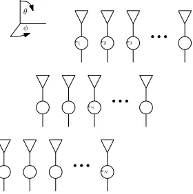
φ θ
[image:1.612.106.246.521.662.2]cn
Fig. 1. Planar array model consisting of elements distributed evenly on x and y axis. Each element have an attached weight.
However the full sacrifice of elevation angle for the sake bandwidth can be avoided by introducing a compromise
between the two through subarray structure. If the array is divided into smaller groups, each subarray can be given a wideband pattern. When superimposed together the overall response will have the common features of the individual subarrays.
II. ARRAYANALYSIS
the time spent for a signal to travel to any point in the antenna structure compared to the reference point is
τ =kr
ω
where k= ω
c
sinθcosφ
sinθsinφ
cosθ
(1)
(2)
Whereωis the angular frequency.θandφare the elevation and
azimuth angles respectively. Thekr represents the projection
of sensor location vectorronto the propagation unit vectork.
When divided by speed of sound, c the projection indicate
time delay τ. Notice that any element distribution can be
represented in equation (1). the The radiation pattern of an
antenna is the resultant of the current excitation I(r) as
follows:
H(ω, θ, φ) =
Z
r∈R
I(r)e−iωτdr (3)
Where R is the set of elements locations. For antenna array
with discrete number of identical elements N with frequency
and angle response D(ω, θ, φ). The array pattern is the sum
of products of the element steering vector elements weights. The above equation the reduces to its discrete form.
H(ω, θ, φ) =
N
X
n=1
D(ω, θ, φ)cne−iωτn (4)
cnis the weighting attached each antenna element with index
n. The following analysis will assume isotropic elements
hence D is omitted.Alternatively for non-isotropic elements
the resultant weighting should divided by the element
re-sponse. cˆn = cDn where cˆn is the effective weighting to
be applied to the element of index n. To use vector format
then the steering vector need to be defined as the set of lag
reference pointrn˙.
s=
e−iωτ1
. . . e−iωτn˙
. . . e−iωτN
(5)
The vector form of array response then becomes
H =
(
cTS ifD= 1
ˆ
cTS otherwise (6)
1) Inverse Discrete Fourier Transform: two dimensional Inverse Discrete Fourier Transform IDFT has been used with rectangular, uniform spacing array to synthesis wideband
beamformer. For planar array, if sensor locationris distributed
evenly on xandy with spacingsdx anddy. For IDFT case,
the element indexing will be separated to the x and y axis
ton andm respectively. Not to be confused with previousn
index. The radiation pattern now reduces to
H = N
2 X
n=−N
2
M
2 X
m=−M
2
cnme−i
ω
csinθ(ndxcosφ+mdysinφ) (7)
Where dx and dy are x and y elements spacings
respec-tively and cnm is the weight attached to the element located
at [ndx, mdy,0]T . From the above equation , two
spatio-temporal variables ωx andωy can be defined as follows
ωx=
ω
cdxsinθcosφ ωy =
ω
cdysinθsinφ (8)
Hence the radiation pattern in terms of newly defined frequen-cies is.
H(ωx, ωy) =
N
2 X
n=−N
2
M
2 X
m=−M
2
cnme−i(nωx+mωy) (9)
Equations (9) above fits the definition of tow dimensional Discrete Fourier transform. It is often desirable to obtain an array response over the frequency band of interest to imitate a
specific pattern, say the desired waveformPd(ω, θ, φ). Desired
pattern is real if array weights are real and can be complex valued if weights are complex. To obtain the required weights for a given desired response, the inverse transformation is applied:
cnm= π
X
ωx=−π
π
X
ωy=−π
Pd(ωx, ωy)ei(nωx+mωy) (10)
Notice that similarity with circular symmetric weighting in [8, p. 259]. Comparing equation (10) with two dimensional DFT approach in [2], [3], [6] reveal that the former is more general and applicable to non uniform and arbitrary shape.
2) Least Squares: Recalll from equation 6 that the array response can be represented in vector format as the product of weights and the steering vector as follows.
H =cTs(ω, θ, φ) (11) The error quantity can be defined as the squared deviation of
the desired pattern Pd from the array response H.
e=Pd(ω, θ, φ)−H(ω, θ, φ) =Pd−cTs
Least square approach minimizes the squared error. Complex matrices are spared by multiplying the matrix buy it is conju-gate transpose. Hence the squared error (SE) becomes:
SE= [Pd−cTs][Pd−cTs]H
= (Pd−cTs)(PdH−sHc∗)
=P2
d −2c
TP
ds+cT(ssH)c
The term Pd s is the correlation vector d and the ssH is
the covariance matrix R. This error is calculated at specific
frequency and angle. To obtain the mean error over the
operating frequency and space, SE is integrated over the
frequency and angles.
M SE=
Z
ω
Z
θ
Z
φ
P2
d −2c
Td+cTRc
= 1−2cTˆd+cTRˆc
apparently squared error is a quadratic function of c. The
least point can be found by differentiating w.r.tcthen finding
the null space of the result [8].
∂
∂cT1−2c
Tdˆ+cTRˆc
= 0−ˆd−0−Rˆc
Hence the set of weights that achieves the least squared error is
c= ˆR−1ˆd (12)
whereRˆ is the integration of the squareNxN covariance
matrix over space and frequency.disNx1 column vector as
follows:
ˆ
R=
Z
ω
Z
θ
Z
φ
R(ω, θ, φ)dωdθdφ
ˆ d=
Z
ω
Z
θ
Z
φ
Pds(ω, θ, φ)dωdθdφ (13)
III. EFFECT OF ASSUMING FIXED ELEVATION ANGLE
Notice that the term ωc sinθ is dependent on both frequency and elevation angle. When defining any desired pattern it is not possible to discriminate between frequency and elevation angle. both parameters can vary according to the following relationship and still produce the same array response.
ω
c sinθ=constant (14)
Near broadside direction the response is less sensitive to angle. This is desirable area for wider frequency band.
IV. ROTATED ELEVATION CONSTRAINT
The phase of array response in (4) depend on both frequency and elevation angle. When defining any desired pattern it is not possible to discriminate between frequency and elevation angle. Both parameters can vary according to the following relationship and still produce the same array response. To resolve the elevation angle ambiguity, Subarrays can be steered to the desired azimuth angle, and then individually rotated around the desired elevation angle. Recall equation (10) used
to calculate array weights. Azimuth angle φinstead of being
constant can be a function of the elevation angle.
ˆ
φm=φ−αm(θ−θ0) (15)
where m= 0, . . . , M
the effect φˆm has on the pattern is to twist the pattern as
elevation angle changes. However, at the desired elevation
angle (θ−θ0) the subarrays align with others. In order to
minimize the total array response in the sidelobe region, the
pattern should be symmetric around φ0. When this balance
is maintained the subarrays cancels each other as long as the
beamwidth is smaller than φˆ−φ0. twist is inflected on the
wavenumber vectorkand its componentsuandv it will then
be as follows.
c ωk(θ,
ˆ
φm) =
ˆ
u
ˆ
v
=
sinθcos ˆφ
sinθsin ˆφ
(16)
To illustrate the effect on the steering matrix lets substitute equation (15) in(16)
k(θ, φm) =
sinθcosφsinβ+ sinθsinφsinβ
sinθsinφsinβ+ sinθcosφsinβ
(17)
whereβ =α(θ−θ0)
Here, β represents the product of subarray slope α and
elevation deviation.
k(θ,φˆm) =
ucosβ+vsinβ usinβ+vcosβ
(18)
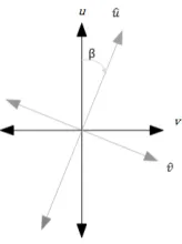
Hence the transformation matrix from the rotated elevation wavenumber to array wavenumber is
ˆ
u
ˆ
v
=
cosβ sinβ
sinβ cosβ
(19)
Equation (19) indicates that as the angleαincreases,ˆumoves
[image:3.612.392.474.58.168.2]away u. Hence, the uvcoordinates rotates with angle α.
Fig. 2. Desired pattern of least square approach at center frequency0.66π
In rotated elevation constraint approach, the constraint is
applied to the elevation angleθ. Recall from equation (1) that
sinθ is common term in both u and v. An incident signal
from elevation angle θ1 and frequency f1 can produce the
same response as another signal from elevation angle θ2 a
andf2 given that they satisfy the following equation:
f1
f2
= sinθ2 sinθ1
(20)
Resulting in beam squint that relates to frequency deviation as
θ= sin−1(sinθ0
f0
f ) (21)
V. POWER CONCENTRATION MEASUREMENTS
Array ability to concentrate power in the desired direction is introduced in [4] as the ratio between power concentration to the total dissipated power into the upper far field hemisphere. The power dissipated over
ψ(ω, θ, φ) =
Z
ω
Z
θ
Z
φ
|H(ω, θ, φ)|2dωdθdφ (22)
The concentrate power can be rewritten as follows.
ρ(ω, θ, φ) = ψ(ω, θ, φ)
Rπ/2
−π/2
Rπ
−πψ(ω, θ, φ)dθdφ
(23)
Substitutingψ in equation (7) results in
ψ(ω, θ, φ) = c
TRˆc
cTc (24)
Where Rˆ is the average sensor covariance matrix calculated
from (13).
VI. SIMULATIONS ANDRESULTS
Concentrated power measurements in this example it is a
cone with 15◦ radius around the reference angle. The wide
one-dimensional azimuth pattern. The elevation is fixed at the
desired elevation angle of 35◦. The array is constructed by 3x3
hexagonal subarrays containing 44 elements each. The look
angle is 0◦ azimuth and 35◦ elevation. The desired response
[image:4.612.336.535.55.187.2]is a Taylor window with -90 sildeobe level. Rotation slope between azimuth and elevation varies between -1.5 and 1.5.
Fig. 3. 3x3 hexagonal subarray used for simulation. Element spacing is 30 cm corresponding to λ2
A. 2-D Invers Descrete Fourier Transform
Individual subarrays pattern is shown below. Each subarray is steered individually by its unique slope. Notice how all subarrays illuminate the desired direction but have different response elsewhere.
−1 −0.5 0 0.5 1 −1
−0.5 0 0.5 1
u
v
−1 −0.5 0 0.5 1 −1
−0.5 0 0.5 1
u
v
−1 −0.5 0 0.5 1 −1
−0.5 0 0.5 1
u
v
−1 −0.5 0 0.5 1 −1
−0.5 0 0.5 1
u
v
−1 −0.5 0 0.5 1 −1
−0.5 0 0.5 1
u
v
−1 −0.5 0 0.5 1 −1
−0.5 0 0.5 1
u
v
−1 −0.5 0 0.5 1 −1
−0.5 0 0.5 1
u
v
−1 −0.5 0 0.5 1 −1
−0.5 0 0.5 1
u
v
−1 −0.5 0 0.5 1 −1
−0.5 0 0.5 1
u
v
Fig. 4. Individual subarray pattern for the 3x3 array being simulated inuv
coordinated described above.
[image:4.612.56.234.153.368.2]IDFT method produced the cleanest mainlobe and relatively low grating lobes over the frequency band.
Fig. 5. 3D normalized magnitude pattern of rotated elevation constraint using IDFT method
rotated elevation method show relatively flat gain over frequency band compared to conventional 1-D approach. This means that grating lobes are small or are from the look direc-tion since they cause sudden change in gain over frequency.
300 320 340 360 380 400 420 440 460 480 500 0
5 10 15 20 25
Frequency MHz
Ar
ra
y
d
ir
ec
ti
v
it
y
d
B
i
Rotated azimuth IDFT 1-D IDFT
Fig. 6. Power concentration comparison between conventional 1-D pattern IDFT synthesis and one using proposed rotated elevation constraint method
B. Least squares
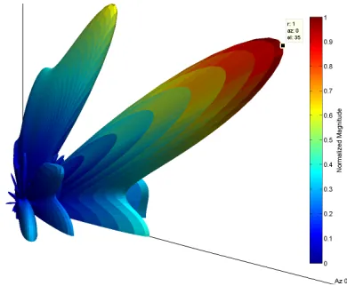
[image:4.612.335.537.289.395.2]Grating lobes are close in magnitude to the main lobe. Grating lobes numbers and locations vary with frequency and their effect can be seen in the gain graph.
Fig. 7. 3D pattern at 400 MHz center frequency obtained by the proposed rotated elevation constraint method using least squares approach
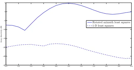
[image:4.612.341.536.500.661.2] [image:4.612.60.290.533.650.2]300 320 340 360 380 400 420 440 460 480 500 −30
−25 −20 −15 −10 −5 0 5
Frequency MHz
Ar
ra
y
d
ir
ec
ti
v
it
y
d
B
i
Rotated azimuth least squares 1-D least squares
Fig. 8. Concentrated power comparison between conventional 1-D pattern synthesis and the proposed rotated elevation constraint method using least squares approach
VII. CONCLUSION
Rotated elevation method provides a compromise for planar arrays between narrowband 2-dimensional space steering and wideband sensor delay line with 1-dimensional steering in azimuth only. This is achieved by dividing the array into subarrays and steer them toward the desired azimuth angle. Then individually rotate each subaarry using a unique slope around the desired elevation angle. Results indicate acceptable gain flatness and power concentration but introduced high grating lobes close to the look direction. Superposition of multiple 1-D smaller arrays caused movement of grating lobes around the mainlobe.
REFERENCES
[1] A. Alshammary. Frequency invariant beamforming using sensor de-lay line. In Electronics, Communications and Photonics Conference (SIECPC), 2011 Saudi International, pages 1–5, 2011.
[2] M. E. Bialkowski and M. Uthansakul. A wideband array antenna with beam-steering capability using real valued weights. Microwave and Optical Technology Letters, 48(2):287–291, 2006.
[3] M. Ghavami. Wideband beamforming using rectangular arrays with-out phase shifting. European Transactions on Telecommunications, 14(5):449–456, 2003.
[4] P. Karagiannakis, S. Weiss, G. Punzo, M. Macdonald, J. Bowman, and R. Stewart. Impact of a purina fractal array geometry on beamforming performance and complexity.
[5] W. Liu. Adaptive wideband beamforming with sensor delay-lines.Signal Processing, 89(5):876 – 882, 2009.
[6] W. Liu and S. Weiss.Wideband Beamforming: Concepts and Techniques. Wireless Communications and Mobile Computing. Wiley, 2010. [7] M. Uthansakul and M. Bialkowski. Fully spatial wide-band beamforming
using a rectangular array of planar monopoles. Antennas and Propaga-tion, IEEE Transactions on, 54(2):527–533, 2006.
[image:5.612.63.290.56.176.2]