A Hybrid Approach of Traffic Flow Prediction Using Wavelet Transform and Fuzzy Logic

University of Windsor University of Windsor

Scholarship at UWindsor

Scholarship at UWindsor

Electronic Theses and Dissertations Theses, Dissertations, and Major Papers

2017

A Hybrid Approach of Traffic Flow Prediction Using Wavelet

A Hybrid Approach of Traffic Flow Prediction Using Wavelet

Transform and Fuzzy Logic

Transform and Fuzzy Logic

Jabed Hossain University of Windsor

Follow this and additional works at: https://scholar.uwindsor.ca/etd

Recommended Citation Recommended Citation

Hossain, Jabed, "A Hybrid Approach of Traffic Flow Prediction Using Wavelet Transform and Fuzzy Logic" (2017). Electronic Theses and Dissertations. 5987.

https://scholar.uwindsor.ca/etd/5987

This online database contains the full-text of PhD dissertations and Masters’ theses of University of Windsor students from 1954 forward. These documents are made available for personal study and research purposes only, in accordance with the Canadian Copyright Act and the Creative Commons license—CC BY-NC-ND (Attribution, Non-Commercial, No Derivative Works). Under this license, works must always be attributed to the copyright holder (original author), cannot be used for any commercial purposes, and may not be altered. Any other use would require the permission of the copyright holder. Students may inquire about withdrawing their dissertation and/or thesis from this database. For additional inquiries, please contact the repository administrator via email

A Hybrid Approach of Traffic Flow Prediction Using Wavelet Transform and

Fuzzy Logic

By

Jabed Hossain

A Thesis

Submitted to the Faculty of Graduate Studies

through the School of Computer Science

in Partial Fulfillment of the Requirements for

the Degree of

Master of Science

at the University of Windsor

Windsor, Ontario, Canada

2017

A Hybrid Approach of Traffic Flow Prediction Using Wavelet Transform and

Fuzzy Logic

by

Jabed Hossain

APPROVED BY:

______________________________________________

K. W. Li

Odette School of Business

______________________________________________

M. Kargar

School of Computer Science

______________________________________________

X. Yuan, Advisor

School of Computer Science

iii

DECLARATION OF ORIGINALITY

I hereby certify that I am the sole author of this thesis and that no part of this

thesis has been published or submitted for publication.

I certify that, to the best of my knowledge, my thesis does not infringe upon

anyone’s copyright nor violate any proprietary rights and that any ideas, techniques,

quotations, or any other material from the work of other people included in my thesis,

published or otherwise, are fully acknowledged in accordance with the standard

referencing practices. Furthermore, to the extent that I have included copyrighted

material that surpasses the bounds of fair dealing within the meaning of the Canada

Copyright Act, I certify that I have obtained a written permission from the copyright

owner(s) to include such material(s) in my thesis and have included copies of such

copyright clearances to my appendix.

iv

ABSTRACT

The rapid development of urban areas and the increasing size of vehicle fleets are causing

severe traffic congestions. According to traffic index data (Tom Tom Traffic Index 2016),

most of the larger cities in Canada placed between 30th and 100th most traffic congested

cities in the world. A recent research study by CAA (Canadian Automotive Association)

concludes traffic congestions cost drivers 11.5 million hours and 22 million liters of fuel

each year that causes billions of dollars in lost revenues. Although for four decades’ active

research has been going on to improve transportation management, statistical data shows

the demand for new methods to predict traffic flow with improved accuracy.

This research presents a hybrid approach that applies a wavelet transform on a

time-frequency (traffic count/hour) signal to determine sharp variation points of traffic flow.

Datasets in between sharp variation points reveal segments of data with similar trends.

These sets of data, construct fuzzy membership sets by categorizing the processed data

together with other recorded information such as time, season, and weather. When

real-time data is compared with the historical data using fuzzy IF-THEN rules, a matched

dataset represents a reliable source of information for traffic prediction. In addition to the

proposed new method, this research work also includes experiment results to demonstrate

v

DEDICATION

First of all, I dedicate this research to my creator almighty Allah. I would also like to dedicate my

research to my mentor, my advisor, my brother Jahid; without whom I wouldn’t achieve whatever

I achieved in my life. I dedicate this research to his parenthood towards me, which gives me the

independence for being a child until the end. I dedicate this research to my parents. My mother

Razia, who always supported me through thick and thin. I dedicate this research to her sacrifices

that she made for me. My father has been the source of motivation for me. I dedicate this research

to his hard work, which inspired me to concentrate more. I dedicate this research to my elder

brother Zakir as well, who has taught me to be able to stay grounded and confident to face any

challenges. Last of all, I dedicate this research to my Moon who gave me peace and always

vi

ACKNOWLEDGEMENTS

I would like to express my deepest appreciation to my supervisor Dr. Xiaobu Yuan for providing me with an exciting opportunity to work in an interesting and challenging field of research. His vision helped me to get innovative in my thinking and also motivated me to research.

My humble gratitude goes to my internal reader Dr. Mehdi Kargar for his extensive support for my research. He has always helped with any of my queries regarding my research. He suggested me with his valuable insights which helped me to improve my research.

I am thankful to my manager at work Jim Reid. He has trusted on me like no one else. He supported me while I was struggling with my research. Without his continuous support, it would have been so much tougher.

vii

TABLE OF CONTENTS

DECLARATION OF ORIGINALITY ... iii

ABSTRACT ... iv

DEDICATION ...v

ACKNOWLEDGEMENTS ... vi

LIST OF TABLES ... ix

LIST OF FIGURES ...x

LIST OF APPENDICES ... xi

LIST OF ABBREVIATIONS/SYMBOLS ... xii

CHAPTER 1 INTRODUCTION ...1

1.1 Transport Management System ... 1

1.2 Traffic Congestion Management ... 5

1.3 Problem Statement and Motivation... 7

CHAPTER 2 ...13

LITERATURE REVIEW AND BACKGROUND MATERIAL ...13

2.1 Input Data in Previous Methods ... 13

2.2 Sources of Data ... 15

2.3 Forecasting Techniques ... 16

CHAPTER 3 ...18

WAVELET TRANSFORMATION ...18

3.1 Signal Processing ... 18

3.2 Mathematical Transformation of Signal ... 19

3.2.1 Fourier Transform ... 20

3.2.2 Disadvantages of Fourier Transform ... 22

3.3 Wavelet Transform ... 23

viii

3.4 Sharp Variation Points ... 27

CHAPTER 4 ...29

FUZZY LOGIC ...29

4.1 Definition ... 29

4.2 Fuzzy Sets and Membership Function ... 31

4.3 Fuzzy Logic System ... 33

CHAPTER 5 ...35

DATA CATEGORIZATION AND DESIGN of ALGORITHM ...35

5.1 Data Categorization ... 35

5.2 Design of Algorithm ... 39

5.2.1 Overview ... 39

5.2.2 Time Complexity ... 44

CHAPTER 6 ...45

EXPERIMENT AND RESULTS ...45

6.1 Overview ... 45

6.2 Experiment Analysis ... 45

6.2 Results and Analysis ... 49

CHAPTER 7 ...54

CONCLUSION AND FUTURE WORK ...54

7.1 Concluding Remarks ... 54

7.2 Future Improvement and Direction ... 54

BIBLIOGRAPHY ...56

APPENDICES ...60

Appendix A ... 60

Appendix B ... 61

ix

LIST OF TABLES

Table 1: Sub-Modules of traffic information system [2] ... 4

Table 2: Canada’s Worst Bottlenecks, 2015 [5] ... 9

Table 3: Performance Measure for Forecasting Occupancy [21] ... 14

Table 4: Performance Measure for Forecasting flow (time) [21] ... 14

Table 5: Advantages and Disadvantages of Previous Popular Methods ... 17

Table 6: Applications of Fuzzy Logic [Kosko at el. [41]] ... 30

Table 7: Chaotic Information Added with Traffic volume/hour. ... 38

Table 8: SVP of different dataset until 9:00 PM ... 46

Table 9: Discrete Difference of Traffic Count Between January 27, 2014 and Other Historical Data ... 47

Table 10: Original and Predicted Traffic Count with the Predicted Date ... 48

Table 11: Forecasting Accuracy for One Hour and Comparison with Traditional Approaches ... 50

Table 12: Prediction Results for Hybrid Approach on Real Data ... 50

x

LIST OF FIGURES

Figure 1: Population Percentage in Urban Centers in Canada [1] --- 1

Figure 2: Main components of classic Transportation Information System [2] --- 2

Figure 3: Major Causes of Traffic Congestion in the US [highway.org] --- 7

Figure 4: Best and Worst Largest Cities for Traffic in Canada (Tom Tom Traffic Index, 2016) --- 10

Figure 5: One-Dimensional Signal (Waveform) --- 18

Figure 6: Two-Dimensional Signal Representing Time-Frequency --- 19

Figure 7: Voice Signal Representing Time and Amplitude [34] --- 21

Figure 8: Fourier Transformation [34] --- 21

Figure 9: Non-stationary Signal Broken into Stationary Sub-signals --- 24

Figure 10: Transformed Signal with Scale Value = 3 --- 26

Figure 11: Transformed Signal with Scale Value = 10--- 26

Figure 12: 10 Sharp Variations Points Alongside Transformed Signal Curve --- 27

Figure 13: Graph Representation of Crisp Set and Inputs (Retrieved from www.mathworks.com) --- 31

Figure 14: Graph Representation of Fuzzy Sets and Inputs (Retrieved from www.mathworks.com) --- 32

Figure 15: Fuzzy Logic System Structure [43] --- 34

Figure 16: Location of The Road on Which The Experiments are Conducted (Retrieved from http://www.wsdot.wa.gov/) --- 36

Figure 17: Wavelet Transformation using Morlet Wavelet Function --- 41

Figure 18: Wavelet Transformation using Mexican Hat Wavelet Function --- 42

Figure 19: Original Signal for Testing Application Accuracy --- 52

Figure 20: Predicted Signal by Hybrid Approach --- 53

xi

LIST OF APPENDICES

Appendix A The following table shows the fuzzy membership sets and their degree of membership compared to the complete set discussed in section 6.2.

60

Appendix B Following Figure shows the vacation calendar of the month of January 2014, retrieved from www.timeanddate.com website.

xii

LIST OF ABBREVIATIONS/SYMBOLS

FFT Fast Fourier Transform

AADT Annual Average Daily Traffic

FT Fourier Transform

WSDOT Washington State Department of

Transportation

CWT Continuous Wavelet Transform

1

CHAPTER 1

INTRODUCTION

1.1 Transport Management System

Urbanization is a process through which population in urban areas increases over a short

period of time; becoming more specialized, which brings socio-economic development in

an urban area. The main reasons behind urbanization are better jobs, fancy lifestyle, more

scope for social interactions and rich cultural diversity etc. According to Statistics Canada,

over 80 percent of Canadians tend to live in urban areas, mostly in the three big cities

Montreal, Toronto and Vancouver [1]. Compared to 1911, when 45% of the total population

used to live in urban cities, 36% more people moved to reside in urban areas making it

81% of the entire population at 2011 [1]. Figure 1 depicts the above information provided.

Figure 1: Population Percentage in Urban Centers in Canada [1]

With all the better perspective of life, urbanization also brings some unavoidable

difficulties to the inhabitants of urban cities. Govt. as well as private sectors have

2

urbanization. City-system includes an economic system, health care system,

transportation system and infrastructure planning e.g.

Traffic condition of a city, if not the most; is one of the most important aspects of

an excellent socio-economic sustainability of an urban area. As nearly all of the people in

any metropolitan area highly dependent on road transportation network for completing

their essential daily functions, traffic information system has always played the most vital

role. Traffic information system involves collecting, categorizing and processing of current

as well as historical traffic data by any govt. or non-govt. organizations to circulate

traffic-related information to the people. Traffic information system mainly consists three key

elements which are traffic related data collection, data processing, information

dissemination [2] which is described in Figure 2.

Figure 2: Main components of classic Transportation Information System [2]

Moreover, this type of management system also involves processing collected data for

prediction of traffic condition, road infrastructure development, substructure planning of

a city, etc. Planned traffic management and control system requires extensive information

regarding operational state and characteristics of traffic flow [2]. Parameters which are

most relevant to traffic management system might include but not limited to [2]:

• Traffic Flow or Volume – the number vehicles crossing a road intersection per unit

3

• Road Information – data regarding a particular road such as geographical

information of the route, number lanes and connected highways;

• Weather Condition – relevant information of weather against traffic flow in a given

time which might include temperature, weather events (snow, rain, wind speed,

fog), etc.;

• Traffic Density – vehicle count occupying a road lane per unit of length in a given

time;

• Incident – an unexpected event that takes place on a particular road which might

impact the flow of traffic in a roadway. Relevant details with this event may

include location, date/time, type of impact, weather condition, number of vehicles

involved, etc. [2]; and

• Time of measurement – time in which count of vehicles and road information is

taken into consideration as inputs to be inputted into the traffic management

system.

These parameters can be measured by using different measurement tools such as

detectors, sensors or can be measured from any vehicle using some vehicle sensors as well

such as speedometer, intelligent heat detector, etc. In spite of having multiple

measurement tools, traffic information system provides a better output if the system is

provided with accurate and robust input.

The traffic information management system is a broad term which consists of

many sub-modules. These sub-modules are developed to achieve different types of

objectives. Table 1 discusses different submodules of traffic management system and their

4

Sub-Modules Description Objectives

Congestion Management Prediction of traffic flow in a

particular time of a day

which helps to come up

with a plan for mitigation of

regular or irregular

congestion.

• Monitoring

congestion in a

particular time at a

day

• Prediction of

congestion

• Road characteristics

prediction

Incident Management Early detection of

unexpected events and

response plan to mitigate

the number of occurrence of

such incidents.

• Unexpected event

detection

• Response Assistance

• Mitigation plan

Traffic Broadcast The process of transmitting

traffic information to

drivers.

• Choosing

unclassified traffic

information to be

broadcasted such as

delays, travel time;

to a driver

• Categorizing road

maps with related

information

Corridor Management Distribution of roads among

vehicles in the same

corridor of road network [2],

e.g. using different routes

from source to destination.

• Finding alternative

routes from source

to destination

• Pre-trip and

en-route advisory [2]

Travel Demand

Management

Improving traffic flow by

managing travel demand [2]

• Congestion Pricing

• Ramp metering

5

1.2 Traffic Congestion Management

One of the most determining sub-module of any advanced transportation management

information system is congestion control. As described in section 1.1, urbanization

provides any metropolitan area with increased number of population which ensures the

fleet size of vehicles increasing time to time. This phenomenon causes vehicle overload in

the road network of an urban area which eventually causes recurrent congestion. Traffic

congestion can be defined as an event in which use of road network increases with

increased number of vehicles characterized by decreased mean speed of vehicles and

increased time in travel. Each street or intersection in a road network has an individual

capability of transporting vehicles. This is defined as the capacity value of the path in a

road network. When the demand passes the capacity value of the road, congestion occurs.

After this kind of condition arises vehicles stays in a particular junction more than the

average time which increases the travel time for any vehicle on that particular road. This

scenario is known as the traffic jam. Such condition can be influenced by weather,

unscheduled phenomenon like accidents, construction, etc. Traffic congestion can be

classified as following,

• Recurring Congestion

• Nonrecurring Congestion

Recurring congestion is known as “peak-hour” traffic. Most of the metropolitan

inhabitants and commuters experience recurring traffic congestion on a daily basis [3].

Recurring congestion is often seen as the capacity problem and logically combated with

raising roadway capacity [3]. People get out of the home in the morning to reach work,

appointments, etc. and at the evening they tend to get back to the house. This circular

process turns highways and major roads into gridlocks [3]. Peak-hour or rush-hour can be

defined as the span of time when the demand from a road crosses the capacity level of that

particular road. Rush hour in a weekday can be entirely different compared to the rush

6

impact of rush hour in the road network. With time the ratio of vehicles on the roads

increases and which causes increased traffic congestion. As the rush hour on weekdays

doesn’t change over time, so the congestion keeps on happening in those times causing

recurring congestion. However, peak hour travel is reinforced by other human tendencies

as well, including school schedules and sleeping pattern [3]. So, peak hour pattern of a

metropolitan city is predictable and keeping this on mind traffic congestion can be

determined.

Unlike recurring congestion which is expected on a weekday or a weekend,

nonrecurring congestion is usually unexpected [3]. Nonrecurring traffic congestion can be

described as traffic delays occurred due to accidental vehicle collision, vehicle breakdown,

road construction, extreme weather, special events, etc. This kind of congestion can

happen during any time of a day due to any number of unexpected events which slows the

traffic. Unlike recurring congestion which is more abstract, nonrecurring congestion has a

more straightforward reason. But sometime nonrecurring congestion follows pattern as

well such as if it is snowing; particular road might face more congestion as vehicles slow

down and create bottlenecks in the main roads of the road network.

While recurring congestion happens to be the main reason behind traffic

congestion, nonrecurring congestion also has a severe impact on traffic congestion.

Therefore, even if recurring congestion is considered to be the main cause of traffic

congestion, nonrecurring congestion needs to analyzed for pointing out the reasons

behind traffic congestion and predicting traffic congestion. Below a graph representation

is presented which shows traffic congestion is equally caused by recurring congestion as

7

Figure 3: Major Causes of Traffic Congestion in the US [highway.org]

The most important requirements for congestion management are predicting the

time of congestion and the volume of vehicles on a particular road. Predicting the time of

congestion helps to define the pattern of recurring and nonrecurring congestion and helps

for planning to identify objectives for congestion management system. Table 1.1 discussed

the goals of congestion management which includes prediction of congestion as well as

road characteristics prediction. Prediction of congestion also provides substantial

evidence for determining rush-hour traffic time and traffic variation between peak hours

and non-peak hours.

1.3 Problem Statement and Motivation

Continuous growth of metropolitan areas in its size of inhabitants and infrastructures are

causing significant drawbacks in the urban transportation system. These disadvantages

8

Traffic congestion has a severe impact on not only the quality of life for the inhabitants of

an urban area but also on the overall economic stability of that area. Productive work

hours, as well as precious personal and family time, are wasted. While shipping

merchandises from one place to another, if it takes longer travel time by trucks, it affects

consumers economically. Lost productivity of the workforce due to the longer travel time

of passenger trips and freight deliveries hinders economic development of the nation.

Delays in travel time, increase fuel consumptions; which are considered as the main

reason behind environmental pollution. In a recent study conducted by Canadian

Automotive Association, it is reported that traffic congestions in the main cities of Canada

cost drivers 11.5 million hours and 22 million liters of fuel each year [5]. Table 2 lists 20

worst bottlenecks of some major cities in 2015 described in the analysis report conducted

by CAA in January 2016 [5]. The report states that the delay in these bottlenecks costs

about $300 million every year [5].

Rank CMA Location Length Annual Total Delay (hours) Annual Delay Cost (mill.) Potential Annual Fuel Savings (liters) 1 Toronto Hwy 401 between Hwy

427 & Yonge St

15.3 3218 82.28 5721 2 Toronto DVP/404 between Don

Mills Rd & Finch Ave

10.5 2174 55.51 3478 3 Montreal Hwy 40 between Blvd

Pie-IX and Hwy 520

10.6 1956 45.60 4197 4 Toronto Gardiner Expy between

S Kingsway & Bay St

7.4 1076 27.51 1671 5 Montreal Hwy 15 between Hwy

40 & Chemin de la CôteSaint-Luc

3.9 812 18.93 1653

6 Toronto Hwy 401 between Bayview Ave & Don Mills Rd

3.3 485 12.40 934

7 Toronto Hwy 409 between Hwy 401 and Kipling Ave

9 8 Montreal Hwy 25 between Ave

Souligny & Rue Beaubien E

2.1 259 6.04 591

9 Vancouver Granville St at SW Marine Dr.

1.6 245 6.08 679 10 Vancouver W Georgia St between

Seymour St & W Pender St

1.2 149 3.70 603

11 Toronto Hwy 401 between DVP & Victoria Park Ave

1.3 143 3.66 395 12 Toronto Black Creek Dr.

between Weston Rd & Tretheway Dr.

0.8 114 2.91 391

13 Toronto Hwy 401 between Mavis Rd & McLaughlin Rd

0.8 103 2.63 164

14 Montreal Hwy 40 between Hwy 520 & Blvd Cavendish

0.9 96 2.23 207 15 Vancouver Granville St between W

Broadway St & W 16th Ave

0.6 88 2.19 276

16 Montreal Hwy 20 near 1re Avenue

0.8 84 1.97 174 17 Qc. City Hwy 73 0.7 78 1.81 127 18 Toronto Hwy 401 interchange at

Hwy 427

0.6 73 1.87 194 19 Toronto Hwy 400 at Hwy 401 0.6 62 1.60 216 20 Vancouver George Massey Tunnel

on Hwy 99

0.6 60 1.50 97 Total 65.2 11546 287 22322

Table 2: Canada’s Worst Bottlenecks, 2015 [5]

The road network which exists in these major cities clearly is not coping with the

increasing demand leading to severe traffic congestion. Nevertheless, construction of new

roads to be added to the road network is time consuming whether now the smartest

solution is using the roads which are already there in the road network. Figure 1.4 presents

10

of the cities are between 30th _{and 100}th _{most traffic-congested cities, and it has been the}

scenario of the last couple of years.

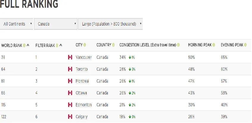
Figure 4: Best and Worst Largest Cities for Traffic in Canada (Tom Tom Traffic Index, 2016)

Since current estimates reveal congestion rate is above normal and might even

grow further, there is always room for new researches regarding management of

transportation. Prediction of congestion being one of the most vital components of such

systems can help to predict future demand which contributes to prevent traffic congestion

using different corridor. Traffic forecast accuracy improves the performance of various

components of transportation systems e.g. corridor management, transit signal priority

control, traveler information system [21]. Prediction process relies on data both historical

and real. Using only real data or only historical data might lead to erroneous prediction as

the traffic tends to exhibit chaotic behavior especially in the metropolitan area [6]. There

are a lot of factors which might influence traffic flow in a particular time e.g. vehicle

collisions, weather conditions, holidays, the day of the week, season, etc. The uncertainty

of data causes uncertainty in the prediction of traffic. Over the years’ scientists have

11

Kalman filter theory [9,10], Markov Chain Model [11], fuzzy-neural approach [12],

sequential learning [13], local regression models [14,15], Bayesian network [16,17], neural

networks [18, 19] and deep learning approach [20] etc. Some of the works combine different methods to come up with a new approach to predict traffic prediction. However,

there is no technique that clearly outperforms any other techniques with the same sets of

inputs in the same experiment environment [6]. More and more research is being

conducted combining two or more methods to predict traffic flow.

This thesis implements a new hybrid approach, combining wavelet transform and

fuzzy logic to predict traffic flow and volume of vehicles using real historical and actual

current data. From a long time, scientists have been using mathematical transformation

on signal to analyze data frequency with respect to time. As traffic data is chaotic, to cope

with the uncertainty of data, fuzzy logic is implemented to turn chaotic characteristic of

data into stochastic behavior. Sharp variation point or zero crossing point has been used

to reveal the similar trend of traffic flow from traffic count per hour. Zero crossing points

refer to the beginning and ending of a trend. So, the window size for taking traffic count is

one hour. For predicting traffic flow in real- time by keeping the integrity of variation

trend, the length of two sharp variation points is reasonable [22].

In the remaining of the thesis, Chapter 2 provides insights of the related works for

prediction of traffic and discusses the data type used to predict traffic. Detail discussion of

the mathematical transformation of time series signal by wavelet transform is presented in

Chapter 3. This remainder of this chapter discusses using Morlet transformation as

continuous wavelet transform and sharp variation points of traffic data to subdivide

similar trend of traffic flow. This chapter also describes the use of scaling functions for

wavelet transformation. Chapter 3 also provides information of some current researches

regarding wavelet transformation which is being used for traffic flow prediction. Chapter 4

mainly describes fuzzy logic systems and the concepts of fuzzy membership sets for

classifying traffic data. Chapter 5 covers data categorization and forming fuzzy

membership sets. The design and implementation of the new algorithm are presented in

this chapter as well. Chapter 6 describes experiment environment, simulation and

12

Results are compared with other related works to demonstrate the proficiency of this new

hybrid approach. Chapter 7 talks about future work and concludes the thesis.

13

CHAPTER 2

LITERATURE REVIEW AND BACKGROUND MATERIAL

2.1 Input Data in Previous Methods

Different approaches use traffic data differently with the dissimilar time span. Some of the

approaches use current data for categorizing and processing those data to predict traffic

volume or traffic speed in the future. For example, Random Walk Forest [7] uses current

traffic conditions to predict traffic flow. On the other hand, methods like Arima Process

[23] reveals short-time traffic conditions of a particular location in the road network based

on previous traffic flow of that particular area. Moreover, there are other methods

presented by R. Chrobok at el. and J. Rice at el. which integrates historical data with current data for classification purposes for forecasting.

Li at el. in his method compares using historical data with both historical and

real-time data to predict traffic congestion [21]. In his paper, Li at el. used 24 data sets with each dataset covering a single day. Each data set contains traffic flow from 5:00 am to

10:00 am and 2:00 pm to 8:00 pm. This method considers two cases for fuzzy rule

construction. In the first case, historical information is being used for constructing fuzzy

rules, while historical and real-time data are used in rule construction in the second case

[21]. The performance of this model is determined by comparing against three commonly

used performance measures for prediction models. They are as followings [2]:

• Mean Absolute Error (MAE) =

∑ ∑I_i=1|x̂_in−x_in|

N

n=1

NI

• Mean Relative Error (MRE) =

∑ ∑ |x̂in−xin| xin I

i=1 N

n=1

14

• Mean Square Error (MSE) =

∑ ∑ (x̂_in−x_in)2

I

i=1 N

n=1

NI

Here, x̂_in represents traffic forecasts at i-1 time for any occupancy level i in n number of run [2]. While N denotes the total number of runs and I indicate the total number of data

points for prediction [2]. Here occupancy means the characteristics of a road being

occupied with vehicles. After the prediction process is completed using fuzzy logic for

both flow (time) and occupancies for all the cases, it is determined that the level of error is

less if the experiment is conducted using both historical and real-time data compared to

using only historical data [2]. Table 3 and Table 4 proves the claim giving conducted

experiment results.

Method Historical Data Only Historical Data combined

with Real Time Data

MRE (%) 12.48 11.97

MAE 1.67 1.54

MSE 8.05 6.71

Table 3: Performance Measure for Forecasting Occupancy [21]

Method Historical Data Only Historical Data combined

with Real Time Data

MRE (%) 5.84 5.61

MAE 5.97 5.75

MSE 65.75 58.49

15

From above method presented by Li at el. [2], it can be suggested that using a combination of historical data with real-time information for prediction traffic situation is

a better approach with marginally improved accuracy. There are also methods developed

on the basis of time series data. For instance, Volterra Neural Network [26] and ARIMA [7]

process attempts to predict the value of a predictable variable based on the previous

values of that variable at a regular interval [6]. Nicholson at el. provided information about the length of dataset [27]. Based on spectral analysis it is an optimal approach to choose

at least 17 days of historical data to predict the future flow of traffic volume [27]. Some

research concentrates only using weekdays data as researchers provided necessary prove

that weekday flow is quite different compared to weekends flow of traffic [27]. Different

factors are considered during prediction of traffic such as,

• different weekdays [24]

• different time periods during the day [27],

• holidays [28]

• special events [24]

• seasonal differences [24] etc.

2.2 Sources of Data

As data is the main requirement for predicting traffic, it is most important to collect traffic

data from trusted sources. The data used in previous researches are collected from Traffic

Management Bureaus, loop detectors, video surveillance camera, GPS-enabled vehicles,

mobile devices, crowdsourcing etc. [6]. Shiliang Sun at el. in his Bayesian approach to predict traffic volume collected data (volume/hr) which was recorded by Traffic

Management Bureau of Beijing [16]. For time series prediction using different neural

networks techniques such as Volterra, RBFNN researchers used volume per hour

techniques on different windows like 15 min, 1 hour. Loop detectors are one of the most

common approaches to collect data for predicting especially short time traffic which is

used by many famous approaches such as CATA, CATB, Slip-Road [29]. A lot of methods

16

conducted using FFT or AADT method to generate synthetic data sets to encounter

information scarcity for predicting traffic volumes as well [22]. Crowdsourcing has become

one of the best approaches to collect data for predicting traffic. Mobile devices have

become really popular. Google Maps uses mobile devices used by people to gather data in

a roadway.

2.3 Forecasting Techniques

Researches on the past used a lot of techniques to forecast traffic volume and congestion

time. Table 5 describes primary methods in the area of traffic flow analysis and traffic flow

prediction with by listing their advantages and disadvantages.

Title Main

Author

Year Advantages Disadvantages Cited By A Bayesian network

approach to traffic flow forecasting

S. Sun 2006 Ability to create Bayesian Network of a traffic flow on a given time by coping with incomplete data

Unexpected conditions such

as events,

holidays,

accidents might

affect the

accuracy

283

Traffic Forecast Using Simulations of Large Scale Networks

R. Chrobok

2001 Real-time data is incorporated, special events are

taken into

consideration

Only used to forecast short time flow

62

Dynamic Prediction of Traffic Volume Through Kalman Filtering Theory

I. Okutani

1984 Short term prediction considering stochastic phenomena with higher accuracy

Bad result in chaotic situation

591

Short-term traffic flow forecasting based on Markov chain model

G. Yu 2003 Short term prediction considering most recent state of traffic which gives better prediction

Can’t forecast

long-term traffic and also fails to produce result during chaotic situation

17

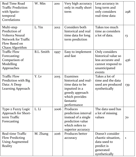
Real Time Road Traffic Prediction with Spatio-temporal Correlations

W. Min 2011 Very high accuracy only in really short term

Less accuracy in long term and only considers real-time data 298 Multi-step Prediction of Volterra Neural Network for Traffic Flow Based on Chaos Algorithm

L. Yin 2012 Considers both historical and real time data for long term prediction

Takes too much time as considers a lot of data. 13

Traffic Flow Forecasting: Comparison of Modelling Approaches

B.L. Smith 1997 Easy to implement and fast

Only considers historical value so less accurate and cannot respond to unanticipated events

436

Traffic Flow

Prediction with Big Data: A Deep Learning Approach

Y. Lv 2015 Examines

historical and real-time data to be inputted in a greedy approach which provides fantastic performance

Takes a lot of time and the data used are produced synthetically

139

Type-2 Fuzzy Logic Approach for Short-term Traffic

Forecasting

L. Li 2006 Produces

prediction interval instead of a single prediction value which refers to superior accuracy

The data used has a lot of missing

values 70

Real-time Traffic Flow Predicting Using Augmented Reality

M. Zhang 2016 Produces better accuracy

Doesn’t consider

chaotic situation, data used to predict is generated synthetically

1

18

CHAPTER 3

WAVELET TRANSFORMATION

3.1 Signal Processing

The world immersed itself with information. Any variable which represents any

information can be denoted as a signal. Examples of signals includes human vocals, the

sound of aeroplane, temperature in a day, human gestures, etc. Human body being a

complex system transmits and receives signals from outside of the body as well as from

inside the body and process those signals to work. Mathematically a signal can be defined

as a real or complex-valued function of one or more variables [32]. Signal varies from one

dimension to multi-dimensions. One dimensional signals represent only a single variable

such as daily mean temperature, annual rainfall etc.; whereas two-dimensional signal

accounts for a function whose domain consists of a two-dimensional real plane such as

time-frequency analysis. Figure 5 and Figure 6 represents a one dimensional and a

two-dimensional signal respectively.

19

Figure 5 represents a waveform signal. This signal can be mathematically represented as,

F(x) = waveform; Here, x is referred as an independent variable.

Figure 6: Two-Dimensional Signal Representing Time-Frequency

Figure 6 represents a time-frequency signal, where x-axis represents time t in a discrete

space (1:00 to 24:00), and y-axis represents the scale of frequency f over that time.

Mathematically this can be expressed as function of both variables,

F(t, f) = F(t) + F(f).

Processing a signal refers to a method by which more useful information can be

revealed from a signal. For example, human hears sound waves and through the auditory

path the brain receives the sound wave and process it to extract information such as low

pitch noise, high pitch noise, etc.

3.2 Mathematical Transformation of Signal

Mathematical transformation is used on signals to obtain further information which is not

readily available on that original signal [33]. This is a way to process the raw signal to

transform into processed signal which provides more information. Most of the signals

Time-20

domain signals represent a graph in which x–axis represents independent variable time

and y-axis represents dependent variable amplitude/frequency [33]. These kinds of graphs

are used to measure frequency on the basis of time. Plotting time-domain signals in a

graph, time-amplitude representation of that signal can be obtained. This kind of

representation does not always provide the best information for any signal processing

related application [33]. In most of the cases, much of the extended information is hidden

in the amplitude of that signal [33]. The frequency spectrum of any signal reveals the

component of the frequency of that signal. This shows characteristics of frequency

components in the signal such as high frequency, low frequency, etc.

Frequency is related to the change of rate of a variable [33]. If a variable change

rapidly with respect to time, we define it to be a variable of high frequency. Whereas if it

does not change rapidly or change smoothly, it is called a variable with low frequency. For

example, if publication frequency of newspaper is considered, daily newspaper has a

higher frequency than the weekly and the monthly newspaper.

3.2.1 Fourier Transform

One of the most famous mathematical transformation used to measure the

frequency component of a signal is Fourier Transformation (FT). FT transforms a

time-domain signal and represents a processed frequency-amplitude signal with one axis being

the amplitude and other representing frequency [33]. An amplitude of a wave can be

defined as the measure of change over a single wave period. This kind of representation

reveals the amount of each frequency existing in the frequency-amplitude signal. For

example, if we consider a voice signal represented Figure 7, we get to know the time along

x-axis and along y-axis we get to know the amplitude of the voice signal, which can be

21

Figure 7: Voice Signal Representing Time and Amplitude [34]

Plotting a signal in the time-domain can be informative, while scientists find it

useful to put a signal in the frequency-domain as well [34]. As discussed earlier, in

frequency-domain representation of graph frequency is represented along the x-axis,

whereas; amplitude is represented along the y –axis. Figure 8 plots a signal in time-domain

and frequency-domain graphs.

Figure 8: Fourier Transformation [34]

The first graph represents the frequency-domain representations of the signal. The three

22

transforming a signal from time-domain to domain and from

frequency-domain to time-frequency-domain can be referred as Fourier Transformation [34]. The amplitude

differs from one frequency to another which represents the different amplitudes and their

frequency. Having FT on signals helps to reduce noise, compress data, detecting changes

in frequencies etc.

3.2.2 Disadvantages of Fourier Transform

Although FT is probably the most used mathematical transformation in this world

for engineering applications, there are lot of other transformations as well such as Wavelet

Transformations, Featured Transformations, Wigner Distribution, etc. Each and every

transformation technique have their advantages and disadvantages with their area of

applications. Fourier Transformation has some drawback of itself as well. Fourier

Transformation has a reversible characteristic which means this technique allows a signal

to go back to its raw signal after being processed and vice verse [33]. But with even if FT

has this characteristic, this technique only can represent one representation either

frequency-domain or time-domain, at a given time [33]. This means, there will be no

frequency information in a time-domain signal and no time information in

frequency-domain signals [33]. As FT is mainly used to reveal frequency information in a

time-domain signal this technique provides the best performance when the signal is stationary

[33]. This technique does not tell in which time that frequency exists. Stationary signal

refers to those signals in which frequency contents do not change over time [33]. For

example, statistics proves that an average of 50 Hz of electricity is needed in each house of

the residents of the USA per day. So, every day the electricity consumed in a house in the

USA is 50 Hz which doesn’t change over time. FT could produce a frequency-domain

representation of this scenario to reveal the frequency of 50 Hz electricity of a house in the

USA. On the other hand, if any house uses 50 Hz, 60 Hz and 70 Hz in consecutive days

using FT won’t provide time-frequency ratio of electricity use for that house which can be

a valuable information to have experimented. Therefore, if time localization of frequency

component for any signal is needed for further investigation time –frequency

23

3.3 Wavelet Transform

Waves can be denoted as oscillation function of time and space such as sine wave or

sinusoid [35]. A wavelet is nothing but a small wave that represents energy (frequency)

with respect to time for providing a tool to analyze non-stationary signals [35]. Wavelet

possesses the ability for analyzing simultaneous time and frequency components of a

signal with strong mathematical foundation [35]. When it comes to signal processing

particular frequency component occurring at any time can provide interesting information

[33]. Wavelet transform can process a raw signal by providing time-frequency

representation of that signal [33].

Fourier Transformation transforms a signal by deconstructing the signal into

waves that are infinitely long [34]. Concentrating on the frequency domain, it becomes

tough to isolate the frequency with respect to time as the frequency with a high resolution

never stops. Recalling the example of the use of electricity at a house in use, it becomes

tough to explain the frequency of using 50 Hz of electricity with respect to time because

this frequency exists all time in the signal. So, the time becomes uncertain fi while

transforming a signal focus is only on the frequency component. To solve this problem, a

signal is deconstructed into small wavelets and then added together to process a newly

transformed signal using wavelet transform [34]. For example, if a signal possesses

frequencies of 1000 Hz, firstly wavelet transform deconstructs this signal by splitting the

signal into half through passing the signal from a high-pass to low-pass filters [33]. This

operation generates two versions of the original signals, one consisting of high-pass

portion (500 to 1000 Hz) and another consisting of low-pass portions. After that, wavelet

transform performs the same task again on those high-pass and low-pass filters until the

original signal is decomposed to a certain level. This process decomposes the original

signal into n number sub-signals where each signal corresponds to different frequency

bands by limiting time [33]. After that wavelet transform adds all the sub-signals and plot

them into a graph to represent time-frequency representation of a graph. Wavelet

transform generally processes a signal in the wavelet domain rather than frequency

domain [34]. The time limiting quality of wavelet transform has proved this technique to

24

the time-domain resolution. For higher frequencies, wavelet transform squishes the wave

together whereas, for lower frequencies it stretches them out. This phenomenon is

handled by the scale parameter of the wavelet [34].

3.3.1 Types of Wavelet Transform

There are mainly two types of wavelet transforms,

I. Continuous Wavelet Transform (CWT) II. Discrete Wavelet Transform (DWT)

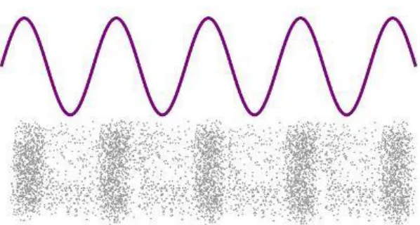
Figure 9: Non-stationary Signal Broken into Stationary Sub-signals

From the concept of wavelet transform it is already being discussed how wavelet

transform decomposes a raw signal into time-limited sub-signals with same frequency

bands. This process is also known as making a non-stationary signal stationary. So, over a small-time period, the frequency spectrum remains unchanged. Figure 9 shows how

25

Hz, 20-80 Hz and 80-120 Hz. Thus, over a period of time, the signal only provides a

time-frequency representation at a maximum 20 Hz time-frequency spectrum and similarly 80 Hz for

the second signal and 120 Hz for the third one. So, in the first signal, the frequency

spectrum remains 20 Hz at all time making it as a stationary signal. Wavelet transform

uses a wavelet function (t) to perform this task, and the transformation is computed

separately for different segments of the time domain signals. Mathematical representation

for Continuous Wavelet Transform can be described as below,

)dt

s

τ

t

(

ψ

x(t)

s

1

s)

,

(

CWT









The above equation represents the transformed signal as a function of two variables. The

first variable is  and the second variable is s, where  can be defined as the translation

and s can be defined as the scale parameter. (t) is the wavelet function.

The scale parameter in the analysis of wavelet is almost identical to scale used in

the Google or Bing map [33]. A high scale in a map corresponds to a less detailed view of

an area and low scale corresponds to a highly-detailed view of an area. Similarly, in

wavelet analysis, low frequency or high scale denotes global information of a processed

signal whereas, high frequency or low scale denotes a local information of a transformed

signal which more detailed and might reveal the hidden pattern of information [33].

Generally, in practical applications, high frequencies do not last through the entire raw

signal whereas, low frequencies last the entire signal. Scaling parameters are mainly used

for either stretching or compressing a signal [33]. So, larger scale stretches the signal, and

small value of scale parameter shrinks the signal. Figure 10 and Figure 11 represents two

transformed signals by wavelet transform (Morlet) with a small scaling and a large scaling

26

Figure 10: Transformed Signal with Scale Value = 3

Figure 11: Transformed Signal with Scale Value = 10

As from the definition of a continuous variable we know that a continuous variable

can be of any value within defined range. For example, time in a race. This variable can be

denoted from minute to nanosecond. The characteristics of this type of pure continuous

behavior of the CWT makes the computation for transforming a signal really time-

consuming. That’s why scientists discretize time for continuous wavelet transform in

order to compute transformation of a signal using a computer [33]. But even after that,

27

hand, transforms a signal revealing sufficient amount of information taking linear

computation time [33].

Discrete Wavelet Transform transforms a signal, using a finite (discrete) number

of wavelet scale parameters and translation variables concentrating on some defined rules

such as a number of coefficients that represents the wavelet. This is the main difference

between CWT and DWT. The scale discretization conducted by CWT is finer compared to

DWT which makes CWT better when it comes to provide more information. This is the

best reason to choose CWT for time-frequency analysis to precisely localize signal

transients.

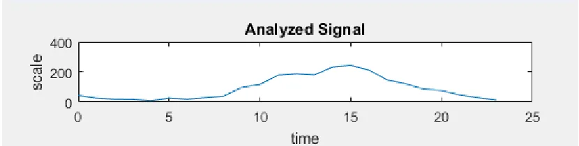
3.4 Sharp Variation Points

Wavelet analysis transforms a signal and represents the processed signal using an

approximation as well as detailed coefficients. After transforming the signal, the wavelet

detail coefficient provides positive and negative values. A zero-crossing point between the

values of detail coefficients represents the sharp variation points in the original signal.

Figure 12 shows the sharp variation points alongside the transformed signal curve.

Figure 12: 10 Sharp Variations Points Alongside Transformed Signal Curve

Signals usually contain high and low frequencies. For low frequencies, the fine

28

frequencies as they vary quickly over time fine time resolution is necessary [37]. Wavelet

transformation uses multiresolution analysis to analyze signal which satisfies the

low-frequency and high-low-frequency characteristics of a raw signal. As for low value of scale

parameter, wavelet transform provides finer detailed information, it becomes easier to

locate special feature of the signal such as sharp variation points. From section 3.3 we

know wavelet transform of a signal can be denoted as,

)dt

s

τ

t

(

ψ

x(t)

s

1

s)

,

(

CWT









Here (t) refers to the wavelet function to transform the signal. If we use Morlet wavelet

function to transform the signal, then (t) can be written as [38],

 2 2 ) ( ψ t ist e e t  

After discretizing scales for transforming a signal, wavelet transform can be represented

as,

)

s

t

n

(

q(n)

s

1

s)

,

Wq(







t

Here, q(n) represents the time series, and n ranges from 1 to N for the whole set vector.

For a particular factor of scale, sharp variation points must satisfy the following condition.

Wq(t, s)Wq(t + 1, s) < 0

The detail coefficients represent values positive and negative. So, the multiplication

between two consecutive coefficients if becomes less than zero then those points will be

29

CHAPTER 4

FUZZY LOGIC

4.1 Definition

The uncertainty of data refers to those data which may contain noise that restricts itself to

provide correct and precise value. Here the term “noise”, can be denoted as observation

error, missing data point, measurement uncertainty, etc. Requiring precision in predicting

systems translates to requiring higher accuracy through collecting noise free data [39].

There are a lot of methods developed to cope with data uncertainty such as

probability theory, the Bayesian network, Markov model, etc. Instead of using real correct

number, probabilities of the value being correct can be employed. In the real world, there

are no certainties among different variables. Thus, it is always a good choice to associate

the probability of correctness or certainty with a particular variable. For example, the

probability of having a disease with the result of a test. Bayesian methods having

advantages like dealing with uncertainty by including prior probabilities have some

disadvantages as well. Bayesian networks don’t work well with missing values thus; it

cannot cope with the real-world changes simultaneously. Many alternative methods have

been suggested to encounter this problem. Fuzzy logic has emerged as one of the most

popular methods to deal with this problem.

Lofti Zadeh at el. first presented the concept of fuzzy logic as a method of processing data by discussing partial set membership opposite to crisp set membership

[40]. Considering all the uncertainties in data, a predictive system does not need to find

precise information but can find close to accurate information considering noisy data as

input. Fuzzy logic is a method that helps a system to arrive to an accurate conclusion

based on imprecise, vague or missing input information [40]. Fuzzy logic implements a

rule-based IF A AND B THEN Z approach to design systems in order to solve problems

rather than modeling a mathematically descriptive solution [40]. Table 7 describes about

30

Product Company Fuzzy Logic Rule

Air Conditioner Hitachi, Sharp, Mitsubishi Prevents too hot and too cold

temperature oscillation and

consumes less power

Elevator Control Fujitec, Mitsubishi Electric,

Toshiba

Reduces waiting time-based on

passenger traffic

Factory Control Omron Schedules tasks and assembly line

strategies

Golf Diagnostic

System

Maruman Golf Select golf club based on golfer’s

physique and swing

Health

management

Omron Over 500 fuzzy rules to track and

evaluate employee’s health and

fitness

Refrigerator Sharp Sets defrosting and cooling times

based on usage [41].

Shower System Panasonic Suppress variations in water

temperature

Cruise Control in

Car

Isuzu, Nissan Adjusts throttle setting to set speed

based on car speed and acceleration

[41]

Copy Machine Canon Adjusts Drum Voltage based on

picture density, temperature and

humidity

Auto Transmission Honda, Nissan, Subaru Selects gear ratio based on engine

load, driving style and road

condition [41].

31

4.2 Fuzzy Sets and Membership Function

While using fuzzy logic for prediction or decision making, set membership is the key to a

system which faces uncertainty. Mathematically a set is defined as the collection of

variables with some definition or domain information. Any randomly selected variable

from a range of values either belongs to the set or does not belong to the set [42]. For

example, let us consider a set of people with a height of 6 feet, who are considered as tall.

Now, the task is to determine whether a person is tall or not considering 6 feet height as

the base height. Therefore, if a person is 6 feet or above he/she is considered as tall and

not tall otherwise. Figure 13 describes this scenario,

Figure 13: Graph Representation of Crisp Set and Inputs (Retrieved from www.mathworks.com)

The membership function µ represents the domain of the set which is 1.0, either a person’s

height is 6 feet so he/she is inside the crisp set or he/she is not. Real world scenario has

been described by sharp-edged membership function for binary operation [42]. But having

32

heights 6´11´´ and 7´11´´. In the real world, both of these persons are tall. On the other

hand, the binary system also cannot distinguish between two individuals with heights

5´11´´ and 6´. The person, having a height of 5´11´´; is tagged as not tall even after he/she

has one-inch difference to be tall. The result is clearly missing ambiguity in this type of

binary system.

The fuzzy set theory solves this ambiguity of the binary system by introducing the

degree of membership to the solution to find the tallness of a person [42]. Figure 14 shows

fuzzy set approach by denoting the degree of membership with a continuous membership

function.

Figure 14: Graph Representation of Fuzzy Sets and Inputs (Retrieved from www.mathworks.com)

The membership function defines the criteria of a person to be tall or not tall. The vertical

axis denotes the value of the height of a person. According to the inclining membership

function, the person having a membership value 0.3 is not tall. But the person having

membership value 0.95 is very tall.

If X is a space of points and a generic element of that space X is denoted by x. So,

33

A membership function can denote a fuzzy set A in space X,

fA(x).

For any value y, the degree of membership is higher if y is close to fA(x) and lower if y is far from the fuzzy set [42]. Membership functions for fuzzy sets can be defined in any way

as long as membership functions follow the fuzzy IF-THEN rules.

4.3 Fuzzy Logic System

According to Boolean logic any variable x in the space X, is a member of F(y) = t if the

value of x is equivalent t. So, either x is a member of F(y) or not. Fuzzy logic is a superset

of traditonal Boolean logic [43]. Fuzzy logic promotes partial membership to encounter

data uncertainty for prediction, thus providing membership values between complete

membership and complete non-membership criteria [43]. Fuzzy Logic System has three

main components which are,

• Fuzzifier

• Inference Engine

• Defuzzifier

Inference engine stores all the fuzzy IF-THEN the rules to check for the degree

Membership of any variable in the same space as of the fuzzy logic set. For example, “If A

is B Then X is Y”. Here the portion “A is B” is known as the antecedent and “X is Y” is

known as the consequence. Fuzzifier inputs crisp sets into fuzzy sets to activate rules [43].

Finally, the Defuzzifier generates output from the input data set. Figure 15 represents a

system design of Fuzzy Logic System (FLS).

34

35

CHAPTER 5

DATA CATEGORIZATION AND DESIGN of ALGORITHM

5.1 Data Categorization

As it has been discussed in section 2.1 that using historical and real-time data provides

marginally better accuracy when it comes to traffic prediction, this thesis also uses

historical data and real-time data to predict traffic volume. Nicholson at el. [27], proposed that 17 days of data are optimal for prediction. So, the test dataset should at least consist of

17 days of historical data which can be used training data sets. For short-term prediction,

well-known method such as CATA, CATB, Slip Road uses 13 hours of data to predict traffic

volume and traffic speed. CATA uses data which is being acquired using loop detectors

with a 5-min span. This process does not encounter stochastic behavior of traffic data. On

the other hand, Volterra Neural network, New Volterra NN and RBF Neural Network

predicts traffic flow by using time series data (24 days from 10 AM to 2 PM and 4 PM to 8

PM). The prediction window size differs from method to method. For example, CATA,

CATB, Slip road can predict traffic volume up to 15 minutes with a 5-min short span. On

the other hand, processes which use time series information tries to predict traffic for long

term such neural network approaches generally predict up to a couple of hours or more.

This thesis used real recorded traffic data provided by Washington State

Department of Transportation (WSDOT), USA. WSDOT determines traffic count data

from most of the roads in the city road network. This research uses traffic count for the

road at Rhododendron, Coupeville on milepost 20:02 point, Eastbound. Figure 16 shows

36

Figure 16: Location of The Road on Which The Experiments are Conducted (Retrieved from http://www.wsdot.wa.gov/)

26 datasets have been collected from WSDOT which represents traffic count/hr for

26 days from the year 2014. 25 datasets have been used as training data and two days of

data have been used for experimental purposes. As the data recorded for volume count per

hour, so this research uses one hour for the prediction window. Therefore, this study

predicts traffic volume per hour in the future at any given time. Prediction for traffic in a

weekday and weekend can be performed in a lot of methods; given the circumstances as

traffic flow differs between weekends and weekdays.

The data collected from WSDOT are classified by adding more chaotic data to

form fuzzy traffic data set. Chaotic information such as, season, the average temperature

in a day, weekday/weekend, weather events, Holidays, Holiday after one day, etc. This

information is chaotic in a way that the information keeps on changing with time. There

37

robust. Three seasons are considered which are Winter, Summer, and Spring. Weather

data depends on the season. Average temperature drops in winter, whereas; it rises in

summer also in Spring. The flow of traffic in weekdays is entirely different compared to

the flow of traffic in weekends. Holidays changes the flow of traffic and coming holiday

might change the traffic condition as well. So, the data is categorized taking into

consideration all the chaotic behavior which makes the frequency of traffic non-stationary

which means flow changes over time. Weather information for the year 2014 is retrieved

from Weather Underground website. Table 7 shows data classification (Chaotic

Information) for prediction of traffic which is being used in this research.

As there are seven extra data components used to make the dataset more robust, a

fuzzy classifier is used to compare real data with stored data with the degree of

membership. From the definition of the degree of membership denoted by µ discussed in chapter 4.2, first the level of preciseness is defined. Three categories of preciseness are

defined which depends on the value obtained from the degree of membership. These

values range from 0 to 1, so the degree of membership can be defined as µ [0,1]. This means, the degree of membership of any historical traffic dataset will be determined on

the basis of similarities between real-time dataset and historical datasets. This degree of

membership can be of any value from 0 to 1. This topic is elaborately described in section