Increasing security of supply by the use of a local power controller during large system disturbances

This is a postprint of a paper published in IEEE Xplore [http://dx.doi.org/ 10.1109/ISGTEurope.2011.6162785] and is subject to IEEE copyright.



Abstract—This paper describes intelligent ways in which distributed generation and local loads can be controlled during large system disturbances, using Local Power Controllers. When distributed generation is available, and a system disturbance is detected early enough, the generation can be dispatched, and its output power can be matched as closely as possible to local microgrid demand levels. Priority-based load shedding can be implemented to aid this process. In this state, the local microgrid supports the wider network by relieving the wider network of the micro-grid load. Should grid performance degrade further, the local microgrid can separate itself from the network and maintain power to the most important local loads, re-synchronising to the grid only after more normal performance is regained. Such an intelligent system would be a suitable for hospitals, data centres, or any other industrial facility where there are critical loads. The paper demonstrates the actions of such Local Power Controllers using laboratory experiments at the 10kVA scale.

Index Terms-- Smart grids, Distributed power generation, Emergency power supplies, Power system reliability, Power system stability, Power quality, Power generation dispatch, Load flow control.

I. INTRODUCTION

HE frequency deviation event which occurred in the UK on 27th _{May 2008 provides an excellent example of a time}

when distributed generation was not used in its most optimal manner [1]. During this event, loss of two major power stations in the UK led to a drop in frequency in three stages over just 4 minutes (Fig. 1):

 first to 49.8 Hz following the loss of a single 345MW unit at a coal power station,

 then to 49.14 Hz following loss of 1237MW (an entire nuclear power station), and a further

This work has been carried out as part of the Rolls-Royce UTC (University Technology Centre) programme.

A. J. Roscoe is with the University of Strathclyde, Glasgow, UK (e-mail: [email protected]).

C. Bright is with Rolls-Royce PLC, Derby, UK. e-mail: [email protected]).

S. J. Galloway is with the University of Strathclyde, Glasgow, UK (e-mail: [email protected]).

G. M. Burt is with the University of Strathclyde, Glasgow, UK (e-mail: [email protected]).

undesirable tripping of 40MW of large generation and 92MW of distributed generation,

 and finally to 48.795 Hz due to the undesired loss of a further 279MW of distributed generation, and a system-wide reduction in the output of thermal power stations due to reduced output caused by the fall in speed of induction motors driving supplies of fuel, water and air.

The fall in frequency was finally arrested by the operation of low frequency protection which disconnected ≈550,000 customers (546MW). Had this action not taken place, network frequency would have quickly fallen further, potentially leading to complete “collapse” of the transmission network.

Fig. 1. Frequency deviation event of 27th _{May 2008 [1]}

The loss of the additional 40+92+279=411MW generation is clearly undesirable because it aggravates an already serious loss of generation. This additional loss of 411 MW ought not to have occurred according to the grid code, which specifies that distributed generation (DG) should remain in service continuously at frequencies down to 47.5 Hz, and remain in service for at least 20s at frequencies down to 47 Hz. [2].

During the frequency deviation event, it is probable that there were many DG units which could have supported the network during this disturbance, but that were not dispatched and lay idle. Examples would be emergency backup generators at hospitals, data centres, or other industrial facilities. Also, such facilities may be able to prioritize their

Increasing Security of Supply by the use of a

Local Power Controller during Large System

Disturbances

Andrew. J. Roscoe, Chris Bright, Stuart J. Galloway, and Graeme. M. Burt,

Member, IEEE

This is a postprint of a paper published in IEEE Xplore [http://dx.doi.org/ 10.1109/ISGTEurope.2011.6162785] and is subject to IEEE copyright.

local loads relatively easily, such that lower priority loads at such demand centres can be shed during disturbances. The local electrical power systems which include these DG units and local loads can be termed microgrids. This paper proposes a way to manage such microgrids during such disturbances, by implementing a microgrid management algorithm called “Local Power Controller” (LPC).

This LPC has many benefits and aims, but the primary focus in this paper is on the ability of the LPC to

 Support the network during frequency disturbances, by dispatching the DG unit and, if necessary, shedding the lowest-priority local loads. This minimizes or removes the need to for low frequency protection to operate. Such low frequency protection disconnects thousands of unsuspecting customers in a wholesale area-by-area manner, without any concern about the importance of loads.

 Maximizing the security-of-supply to the local high-priority loads, initially by supporting the network as above, but also, should the network subsequently collapse, seamlessly transferring to islanded operation. This makes the local microgrid immune to any subsequent collapse of the transmission & distribution network.

This paper describes the way in which the LPC supports the network, prioritises loads and maximises the security of supply. The paper also describes laboratory experiments on a 10 kVA microgrid which confirms that LPC works in practice.

II. LOCAL POWER CONTROLLER (LPC)

The LPC algorithm in its entirety is a relatively complex piece of software containing a suite of control and protection algorithms, executing on a single processor card.

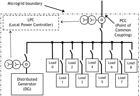
At its highest level, the LPC oversees the control of a microgrid which consists of a local DG unit and local loads (Fig. 2). The LPC has control of local loads by being able to shed loads on a priority basis. In this paper, the load circuits are treated as numbered 0 to 8 in each microgrid, whereby load 0 is the highest-priority load such as a hospital operating theatre or a central computer, and load 8 contains low-priority machines such as air conditioners and coffee machines which can tolerate interruptions to supplies without serious impacts on safety, financial performance, and convenience. Load branch 0 is “always on” while load branch 8 is the first to be shed if shedding is required.

During normal daily operations, the LPC at each microgrid would keep all local load branches connected, although within the load branches various energy pricing or management strategies might actively modify the demand according to price or other network signals, for financial reasons. [3] [4] [5]

Fig. 2. LPC (Local Power Controller) concept for microgrid management Also, during normal daily operations, the LPC could make an informed decision upon whether to despatch the local DG unit or not, at various times of the day, based upon knowledge of prices and constraints [6], such as:

 Maximum microgrid import constraint (power limit), or penalty price per MWh for straying above this limit.

 Maximum microgrid export constraint (power limit) or lowered (or negative) export price per MWh for straying above this limit.

 Price of electrical import within normal import limit.  Price of electrical export within normal export limit.  Price for operating DG unit at different output levels

(overheads plus fuel consumption)

 Price for simply leaving the DG unit standing idle (capital depreciation)

The philosophy of the LPC is that is can be configured with information concerning the above parameters, and then be left to operate in an entirely autonomous mode. Clearly, where power prices or constraints change in real time, there is benefit in passing this information to the LPC via a low-bandwidth communication channel from some higher-level central “control system”, or even a manual user interface. However, the rationale is that should such communications fail, the LPC will remain in an intelligently operating condition using the last set of valid data. Further enhancements of LPC might detect the loss of communications with a higher-level control system, and revert to a pre-set conservative set of parameters which optimise the security of supply or running costs as far as possible, in the absence of outside information.

Within this paper, the scenario described in detail is when the price of imported electricity is lower than the cost of locally generated power from the DG unit, which might require using diesel or hydrogen fuel. This would occur, commonly, when plenty of wind power was available, and demand was not at peak levels. Therefore, the DG units are not dispatched by the LPCs during normal operation.

LPC (Local Power Controller)

Load 0 Microgrid boundary

PCC (Point of Common Coupling)

Load 2

Load

4 Load 6 Load 8

Load 1

Load 3

Load 5

Load 7 Distributed

This is a postprint of a paper published in IEEE Xplore [http://dx.doi.org/ 10.1109/ISGTEurope.2011.6162785] and is subject to IEEE copyright.

This particular scenario is presented since it presents the greatest challenge to LPCs and DG units when a sudden network disturbance occurs, because the DG units are not already dispatched, and need to start “from cold”. In other disturbance scenarios, where the DG units are already dispatched, the response is easier to manage since the DG units are already running and synchronised to the distribution grid.

As shown in Fig. 2, the LPC requires currents and voltages to be measured at just two local points: at the DG terminals, and at the point of common coupling (PCC) to the distribution grid (the boundary of the microgrid). From these measurements (which use algorithms based on those in [7]), the DG power output and grid infeed can be monitored, and the total local load power can be deduced. Also, these measurement points allow the “performance level” (PL) of the DG and grid to be assessed. The term “performance level” (PL) is used here instead of the term “power quality”, since power quality usually refers to fluctuations in the voltage, the voltage waveform, and the phase balance of the electricity supply. In this paper, PL is defined by monitoring the positive-sequence voltage magnitude, and frequency, on a per-unit basis, at both measurement points. A PL score of 0 to 6 is assigned to these two points, (with 6 representing good/nominal and 0 representing very poor), depending upon how close to nominal the values are. Table I shows how the PLs are defined in this paper, although the exact definitions are configurable and may be varied in different scenarios or to support specific grid codes. In future, it would be relatively simple to include measures of unbalance, harmonics, flicker etc. into the PL assessment.

LPC has control over the DG unit and all the contactors in Fig. 2. For traditional synchronous generators coupled to mechanical prime movers, LPC can include all the governor and AVR controls within its functionality, saving cost. Where the DG is more complex, such as an inverter, some of these controls are devolved to a lower-level controller which may need to operate at a very high frame rate to control inverter switching cycles.

By continually monitoring the PL (performance level) at the two key points, the LPC follows a state-table approach to transition from one operating mode to another. There are many different state transitions possible, but in this paper there are a few key transitions which are the most relevant in the discussed scenario. These are summarised in Table I and described below:

TABLEI

EXAMPLE OF STATE TABLE WHEN DG IS DESPATCHED ONLY TO ENHANCE SECURITY OF SUPPLY, I.E. WHEN IMPORTED ENERGY FROM THE GRID IS CHEAP.

1) If the DG unit is not already running due to economical reasons, but is allowed to operated in islanded mode, and grid frequency drops below 49.75 Hz, then the PCC PL drops from 6 to 5. This triggers a “level 1” support mode and the DG unit is started and synchronised with the grid, and outputs lower levels of active and reactive power with conventional droop slopes on frequency/P and voltage/Q (P and Q representing active and reactive power respectively).

2) If the frequency of the grid infeed drops below 49.0 Hz then the PCC PL drops further to 3, triggering a “level 2” support mode which can be called a “virtual island” [8]. Lower priority loads are shed sequentially until the local load magnitude is within the capability of the DG. At the same time, the active power output of the DG unit is adjusted so that is equal to the local load demand. This results in a net zero active power flow across the microgrid-to-grid boundary. This can present a severe risk of non-detection of Loss-of-Mains (LOM) by operating in the non-detection-zone (NDZ) [9],[10], but this risk can be removed by deliberate maintenance of a small managed reactive power flow across the boundary [11]. In this state, the microgrid supports the wider network by reducing its power demand to zero, and can also provide additional stability through the inertia (real or synthetic) of the DG unit. Also, the microgrid is well positioned for any subsequent transition to an islanded state, either forced by a LOM event (due to system collapse and “blackout” of the local distribution grid), or a deliberate transition determined by the LPC.

3) If the frequency of the grid infeed drops below 47 Hz, then the PCC PL drops from 3 to 2, and LPC will deliberately open the contactor between the microgrid and the distribution grid, and form a

This is a postprint of a paper published in IEEE Xplore [http://dx.doi.org/ 10.1109/ISGTEurope.2011.6162785] and is subject to IEEE copyright.

local power island. At this point, the DG control changes from the P/Q control mode to a frequency/voltage control mode. The droop slopes for frequency/P and voltage/Q are modified, so they are suitable for islanded operation. In particular, a non-linear droop slope for frequency/P is used so that generally, power quality (frequency) is held as near nominal as is practical. However if the main DG unit is close to its maximum power output, frequency droop is higher, thereby requesting power from any other (smaller) generators within the microgrid.

4) Later, if the wider transmission distribution grid recovers, such that the PL at the PCC rises all the way to PL 5 (49.5 Hz), then the LPC will initiate a re-synchronisation procedure. Following synchronisation of the microgrid to the distribution grid, the local loads can be reconnected sequentially until all are reconnected. The DG unit remains in a “level 1” support mode.

5) If grid frequency continues to recover above 49.75 Hz, the PL rises further to 6 and the DG unit can also be stood down after a time (unless it is financially sensible to continue to operate it).

An important part of the state-table approach is the hysteresis included between the “entrances” and “exits” of the some of the operational modes. For example, grid frequency needs to drop to 47 Hz to trigger a deliberate transition to islanded mode, whereas grid frequency must recover all the way to 49.5 Hz to initiate a re-synchronisation process. Such an approach is imperative, to avoid cyclic and oscillating behaviours, since transmission and distribution grid is not an infinite bus, and can be affected by the actions of microgrids. Also, it would be wise to wait until the system frequency is within statutory limits in order to avoid connection to a system that might still be weak and at risk of collapse.

It should be noted that Table I shows only a subset of the entire LPC state table:- the subset which is relevant in the described scenario where the DG is only despatched to improve the security of supply. In other scenarios where the DG unit is used in a grid-connected fashion even in cases of good power quality, due to high grid import costs or power-flow constraints, the state table is modified. It should also be appreciated that while the state table forms the core of the decision logic within the LPC, the entire LPC software is a significant piece of software which contains many measurements, calculations, threshold detectors, logic gates, latches, etc., the low-level details of which are beyond the scope of this paper.

The effects of power-system interactions and hysteresis must be carefully considered when implementing a

load-shedding algorithm for use within small or islanded power systems. If fixed frequency set-points are used to trigger the shedding and re-connecting of different load branches, then great care must be taken to ensure that the there is a sufficient hysteresis band between the shedding frequency(ies) and the reconnection frequency(ies). This is because, for example, shedding a single load branch which accounts for 0.2pu of the generator rating, where a 4% frequency droop slope is used, will result in a frequency rise of 0.4 Hz in a 50 Hz system. Therefore, hysteresis bands need to be set with some knowledge of the maximum quantity of load likely to be present within each load branch, and the droop slope in use. Due to the large impact that each load branch can have on the islanded power system frequency, LPC does not use a predefined set of graduated frequency points, one for each load branch. Instead, essentially a single lower frequency is defined which defines the shedding of all load branches, but these are shed one at a time in succession until the limit is no longer violated. In the same way, a single upper frequency point is defined which allows load branches to be reconnected in succession. The minimum allowable hysteresis band between the lower and upper frequency thresholds is defined by the product of:

 nominal frequency (50 Hz in this case)

 the frequency droop slope (p.u. frequency change for 1 p.u. power output change)

 the maximum per-unit load power expected in any single load branch

An extra subtlety is that loads are only disconnected and reconnected at a certain rate, to allow the power system to settle subsequent to each switching event. This is important, otherwise all loads would be shed or reconnected within a very short time. This in turn presents the risk that during severe overloads (sudden and unexpected transitions to islanded mode might cause this), the loads might not be shed quickly enough to avoid a complete frequency collapse due to the limit inertia in the generation unit. Therefore, there are in fact two lower frequency limits. Violation of the upper limit only causes shedding at the normal timer-qualified rate, and only if ROCOF (rate of change of frequency) is negative. Violation of the lower limit (and if ROCOF is negative) causes loads to be shed with a much smaller time limit between successive disconnections. This lower frequency limit can be set slightly above the frequency which would result from the frequency droop slope with the generator outputting its full 1pu rated power, because if frequency settles to this value, the power system is on the verge of collapse.

This is a postprint of a paper published in IEEE Xplore [http://dx.doi.org/ 10.1109/ISGTEurope.2011.6162785] and is subject to IEEE copyright.

thresholds most appropriately.

However, LPC always has a direct measurement of the total local load power, by adding the measurements of generator output power and grid import power in Fig. 2. LPC also knows the capacity of the generator unit. By using this information directly, LPC could implement a much simpler load-shedding algorithm based directly on comparisons of the actual load power against the generator capacity. This would avoid the requirement to wait for the system to settle after each successive load shed or reconnect, and would significantly reduce the time required between the steps, potentially to a time as short as a single cycle, if active power is measured over a single cycle. Further, it might be possible for LPC to learn the likely powers within each load branch from historical measurements. This might mean that load branches could be shed in groups very quickly during sudden islanding events, in order to minimise the frequency disturbance to the remaining critical loads. An even smarter load-shedding algorithm might be able to account for load branches which actually appear to include net generation, and should not be shed.

Note that if instrumentation was inserted on every load branch, the load-shedding algorithm could use this information to aid the decision-making process. However, the present rationale of LPC is to use the minimum possible instrumentation, in order to minimise installation cost and reliability. Therefore, these alternative load-shedding algorithms have not yet been implemented, but might in the long term be significantly beneficial to such islanded systems.

III. PRACTICAL DEMONSTRATION

To demonstrate the proposed functionality of the LPC algorithm, it is coded in MATLAB® _Simulink® _{and converted}

to „C‟ code using the Real-Time-Workshop toolbox. The algorithm manages all software functions, from sampling of the AC voltage and current values, through measurements [7], and high-level decision functions. Practically, in the laboratory the LPC algorithms are executed on an MVME5100 or MVME5500 processor card [12] embedded with a multi-processor rack [13] which enables logging of the performance during complex scenarios. In real applications, many other industrial controller platforms could be used.

The demonstration network (Fig. 3) consists of 2 microgrids which can be connected to a synthetic distribution grid. This grid is provided by an 80kVA synchronous generator which is accurately controlled [14]. In the presented scenario, the grid frequency and voltage follows the following profiles:

 Frequency and voltage ramping from 50 Hz and 1.0 pu to 46.5 Hz and 0.95 pu over 45 seconds, representing a 0.08 Hz/s collapse, the same rate as the greatest change in frequency on 27th _{May 2008}

but extended to the point where the entire transmission grid might fail.

 The “outage” is held for 20 seconds

 Grid frequency and voltage then recover to nominal over 120 seconds.

Fig. 3. Laboratory demonstration of 2 microgrids controlled by LPCs Notably, this scenario contains a quite sudden degradation of frequency, which might easily be seen in practice due to events such as [1]. The “outage” and recovery phases, however, have been sped up for demonstration purposes, and might take much longer in practice for large power networks.

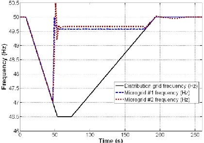
The frequencies of the grid, microgrid #1, and microgrid #2, are shown in Fig. 4. In this scenario, the DG units are switched off at the start. Both are switched on by the LPCs at t=12.5s, 1 second after the 49.75 Hz threshold is violated.

Fig. 4. Frequencies of grid, microgrid #1, and microgrid #2

The two different designs of generator take different times to synchronise. The synchronous generator needs to be physically spun-up and synchronised, which takes nearly 20 seconds, occurring at t=32s (Fig. 5). Also, its prime mover would need to be started from cold which will limit the startup time achievable. The inverter itself can be very quick to start up, in theory almost instantaneous. In this case it takes 9.5s, becoming synchronised at t=22s. However, this requires the energy source supplying the inverter to start equally quickly.

LPC

DG

(Synchronous) Loads Microgrid #1

LPC

DG

(Inverter) Loads

~

This is a postprint of a paper published in IEEE Xplore [http://dx.doi.org/ 10.1109/ISGTEurope.2011.6162785] and is subject to IEEE copyright.

Fig. 5. DG and local load powers: microgrid #1 and microgrid #2

Fig. 5 shows the local load and DG output powers, scaled so that each is in “per-unit” (pu) relative to their respective microgrid DG rating. This is a challenging scenario in which the frequency drop on the grid is so fast that the grid frequency passes the 49.0 Hz threshold at t=21.3s, which is before either DG unit has synchronised. This frequency fall is more severe that that suffered in the incident on 27 May 2008 but could be a credible system condition for example following the islanding of a part of the system in which the load greatly exceeds generation.

This fast fall in frequency initiates the “level 1” support mode, but by the time the DG has synchronised, both LPCs have entered their “level 2” support mode (“virtual islanding”). Therefore, in Fig. 5, it can be seen that the local loads are sequentially shed in both microgrids from t=21.3s, until the total load is less than 1pu.

Since “level 2” support mode is already engaged when the DG units synchronise, the LPC immediately despatches them to export the same active power as the local loads, and this is clearly seen on Fig. 5, leading to net zero active power exchanges with the grid. Since there is a significant risk of non-detection of LOM, a small reactive power exchange is maintained so that LOM can always be detected within 2 seconds as per [15].

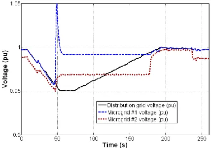
At t=47.2s, grid frequency falls past the 47 Hz threshold, and both LPCs deliberately island their microgrids from the grid. Some momentary power adjustments are seen immedaitely afterwards. This is due to the readjustment of frequency and voltage from the grid levels to the new stable islanded levels. The frequency and voltage supplied to the local loads is shown in Fig. 4 (frequency) and Fig. 6 (voltage). The brief voltage excursion to 1.05pu visible for microgrid #1 is due to the previous (surplus) reactive power required to avoid the LOM NDZ and the time required for the AVR and machine field to settle to the new islanded state. This feature is not evident on microgrid #2, mainly because the inverter is much faster to respond. Of note is that on both microgrids, the DG output active powers were pre-matched to the local load active powers, and so the generators are able to seamlessly ride-through the transition from grid-connected to islanded operation without under/overfrequency or under/overvoltage events, apart from a small, brief voltage disturbance which

would be perceived as flicker.

Once in the islanded state, between t=50s and t=170s when the grid is “down”, the microgrids could sustain themselves as long as their is sufficient fuel for the DG units. Should local load increase or decrease, the load shedding algorithm continues to adjust to ensure that the generator is serving as many loads as possible, without becoming overloaded.

Fig. 6. Voltages at local loads: microgrid #1 and microgrid #2

At t=176s, the grid frequency recovers, evidenced by its frequency rising above 49.5 Hz . Therfore, both LPCs begin a resynchronisation process. In this case, there is no particular urgency to synchronisation, and so this is done in a controlled manner to avoid undue transients in case the local loads include frequency-sensitive or high-inertia devices. The time taken is “random” and depends upon the initial differences in phase and frequency between the microgrids and the distribution grid. In fact, such “random” reconnection might be highly beneficial so that many microgrids do not connect at the same time and coincidentally disturb the distribution grid. Once re-synchronisation is achieved (t=187s for microgrid #1, t=236s for microgrid #2), the local loads which were shed are sequentially reconnected (Fig. 5). Also, in this case, the DG units are stood-down rapidly since the original scenario was that their fuel cost did not justify running simply to export power to the grid. In reality, prudence might dictate that this action might be delayed by minutes or hours, in case the distribution grid is still subject to disturbance.

IV. CONCLUSIONS

The operational strategy presented in this paper demonstrates that both network support functions and local security-of-supply can be improved by allowing DG units to make seamless transitions between grid-connected and islanded operational and vice-versa. This allows “emergency backup” generators to be used in grid-connected scenarios, and “grid-connected” generators to be used in islanded scenarios. While both of these use cases tend to be discouraged by present regulatory frameworks, the potential advantages during scenarios such as May 27th _{2008 should be}

This is a postprint of a paper published in IEEE Xplore [http://dx.doi.org/ 10.1109/ISGTEurope.2011.6162785] and is subject to IEEE copyright.

to the highest priority loads, and to the removal of the need to disconnect unsuspecting customers in their entirety.

The potential impact on the higher-level network and between multiple microgrids warrants further investigation, via more complex simulation studies or power hardware-in-the-loop experiments [16]. This is particularly true where the size of the high-level network is limited, such as a small island or a marine power system, or where the number and size of LPC-equipped microgrids is so large that they become a significant part of the total power system.

V. REFERENCES

[1] National Grid, "Report of the National Grid Investigation into the Frequency Deviation and Automatic Disconnection that occurred on the 27th May 2008," 2009 Available: http://www.nationalgrid.com/NR/rdonlyres/E19B4740-C056-4795-A567-91725ECF799B/32165/PublicFrequencyDeviationReport.pdf, accessed Feb 2010.

[2] National Grid, "The grid code," Issue 4 Revision 6, 2011. Available: http://www.nationalgrid.com, accessed May 2011.

[3] A.-H. Mohsenian-Rad, V. W. S. Wong, J. Jatskevich, R. Schober, and A. Leon-Garcia, "Autonomous Demand-Side Management Based on Game-Theoretic Energy Consumption Scheduling for the Future Smart Grid," IEEE Transactions on Smart Grid, vol. 1, pp. 320-331, 2010.

[4] D. Westermann and A. John, "Demand matching wind power generation with wide-area measurement and demand-side management," IEEE Transactions on Energy Conversion, vol. 22, pp. 145-149, Mar 2007.

[5] A. J. Roscoe and G. Ault, "Supporting high penetrations of renewable generation via implementation of real-time electricity pricing and demand response," IET Renewable Power Generation, vol. 4, pp. 369-382, 2010.

[6] H. A. Gil and G. Joos, "Customer-owned back-up generators for energy management by distribution utilities," IEEE Transactions on Power Systems, vol. 22, pp. 1044-1050, Aug 2007.

[7] A. J. Roscoe, G. M. Burt, and J. R. McDonald, "Frequency and fundamental signal measurement algorithms for distributed control and protection applications," IET Generation, Transmission & Distribution vol. 3, pp. 485-495, May 2009.

[8] A. J. Roscoe, R. C. Knight, and D. R. Trainer, "Distributed Generation (A micro-grid control system including an automatic “Virtual Islanding” mode)," International patent application WO2010130583 (A2/A3), 2011.

[9] Z. H. Ye, A. Kolwalkar, Y. Zhang, P. W. Du, and R. Walling, "Evaluation of anti-islanding schemes based on nondetection zone concept," IEEE Transactions on Power Electronics, vol. 19, pp. 1171-1176, Sep 2004.

[10] A. Dyśko, C. Booth, O. Anaya-Lara, and G. M. Burt, "Reducing unnecessary disconnection of renewable generation from the power system," IET Renewable Power Generation, vol. 1, pp. 41-48, Mar 2007.

[11] A. J. Roscoe, "An electrical generator network and a local electrical system (Power flow management to avoid the non-detection of loss of mains (islanding), relays)," International patent applications EP2286499 (A1), WO2009150397 (A1), US2011068631 (A1), 2011. [12] Emerson Network Power, "MVME5500 VME with PowerPC

Processor," Available: http://www.emersonnetworkpower.com, accessed January 2011.

[13] Applied Dynamics International, "Real Time Station (RTS)," Available: http://www.adi.com, accessed January 2011.

[14] A. J. Roscoe, I. M. Elders, J. E. Hill, and G. M. Burt, "Integration of a mean-torque diesel engine model into a hardware-in-the-loop shipboard network simulation using lambda-tuning," IET Electrical Systems in Transportation, vol. 1, pp. 103-110, 2011.

[15] IEEE, "IEEE Standard for Interconnecting Distributed Resources with Electric Power Systems," IEEE 1547-2003, 2003.

[16] A. J. Roscoe, A. Mackay, G. M. Burt, and J. R. McDonald, "Architecture of a network-in-the-loop environment for characterizing AC power system behavior," IEEE Transactions on Industrial Electronics, vol. 57, pp. 1245-1253, 2010.

VI. BIOGRAPHIES

Andrew J. Roscoe received the B.A. and M.A. degree in Electrical and Information Sciences Tripos at Pembroke College, Cambridge, England in 1991 & 1994. Andrew worked for GEC Marconi from 1991 to 1995, where he was involved in antenna design and calibration, specialising in millimetre wave systems and solid state phased array radars. Andrew worked from 1995 to 2004 with Hewlett Packard and subsequently Agilent Technologies, in the field of microwave communication systems, specialising in the design of test and measurement systems for personal mobile and satellite communications. Andrew was awarded an MSc from the University of Strathclyde in 2004, in the field of “Energy systems and the Environment”, and received his Ph.D degree in 2009. Andrew is currently a Research Fellow in the Institute for Energy and the Environment, Department of Electronic and Electrical Engineering at Strathclyde University, working in the fields of distributed and renewable generation, active network management, power system metrology, inverter control, and marine and aero power systems.

Chris Bright received a BSc degree in electrical engineering at the University of Southampton, UK in 1980 and received an MPhil degree in induction motor control from the University of Southampton in 1987. From 1982, Chris worked in the UK electricity supply industry in research and development and also electrical system design of systems from 415 V to 400 kV, specialising in electrical system protection. Since 2005, Chris has worked in the Rolls-Royce Strategic Research Centre in Derby, UK as an electrical systems specialist.

Stuart J. Galloway received his BSc (honours) in Mathematical Sciences from the University of Paisley in 1992. He was awarded an MSc in Non-Linear Modelling from the University of Edinburgh in 1994 and received his PhD in applied mathematics in 1998. He joined the Electronic and Electrical Engineering Department at the University of Strathclyde in 1998 to work on large scale optimisation problems. He is currently a Senior Lecturer in the Institute for Energy and Environment at the University of Strathclyde. His core research interests spans aero electrical, marine electrical and energy electrical activities and includes strategic and applied research.