N.J. Mottram∗
Department of Mathematics and Statistics, University of Strathclyde, Livingstone Tower, Glasgow G1 1XH, U.K. C.J.P. Newton
Peartree Cottage, Little London, Longhope, Gloucestershire GL17 0PH, U.K.
This paper aims to provide an introduction to a basic form of theQ-tensor approach to modelling
liquid crystals, which has seen increased interest in recent years. The increase in interest in this type of modelling approach has been driven by investigations into the fundamental nature of defects and new applications of liquid crystals such as bistable displays and colloidal systems for which a description of defects and disorder is essential. The work in this paper is not new research, rather it is an introductory guide for anyone wishing to model a system using such a theory. A more complete mathematical description of this theory, including a description of flow effects, can be found in numerous sources but the books by Virga and Sonnet and Virga are recommended. More information can be obtained from the plethora of papers using such approaches, although a general introduction for the novice is lacking. The first few sections of this paper will detail the development
of the Q-tensor approach for nematic liquid crystalline systems and construct the free energy and
governing equations for the mesoscopic dependent variables. A number of device surface treatments
are considered and theoretical boundary conditions are specified for each instance. Finally, an
example of a real device is demonstrated.
I. BACKGROUND
In all matter, the physical state of the material can be described in terms of the translational and rotational motion of the constituent molecules. In a crystalline solid the intermolecular forces hinder motion and force the molecules to lie, on average, in a regular array (i.e. in a crystal lattice structure). As the substance is heated the molecules gain kinetic energy and large molecular vibrations break the crystal structure resulting in a fluid phase. In the liquid fluid phase the intermolecular forces are still strong over the average distance between molecules but cannot maintain the crystal structure. In the gas fluid phase the average distance between molecules is large, the intermolecular forces are weak and the unrestricted motion of the molecules cause the gas to expand and fill the container holding it.
In certain materials, which typically consist of either rod-like or disc-like molecules, it is not just the translational motion, i.e. the motion of positions of the centres of mass of the molecules, which determines the state of matter. We must also consider the orientation of the rod- or disc-like molecules. In a “normal” liquid, or more correctly, an isotropic liquid, the orientation of the molecule is random. If we pick a single molecule and consider how the orientation varies with time it will eventually take all possible orientations. Alternatively, if we look in a small region of the material (say a fixed ball,B, centred at the pointx, see Fig. 1(a)), then the molecules in the ball will be randomly oriented. Such a system, in which a time average is equivalent to a space average, is said to beergodic.
However, in a temperature region between the isotropic liquid and crystal states, some materials exhibit an amount of orientational order. That is, if we look in the small ballBthe orientation is not random, rather there exists an average orientation, see Fig. 1(b). Materials which exhibit such orientational order are calledliquid crystals.
A. Measures of orientational order
For such a situation we can define a unit vector ncalled thedirectorto be the average molecular orientation direction. For rod-like (or calamitic) molecules this will be the average long axis orientation and for disc-like
∗author for correspondence: [email protected]
(a) (b)
B
B
+δ
[image:2.612.191.415.75.176.2]B
-δFIG. 1: A snap-shot of molecules within the ballBin (a) the isotropic liquid phase and (b) the nematic liquid crystal
phase. Due to the head-tail symmetry of the molecules, the order parameter integration need only be performed over the half sphereδB+orδB−.
0 f(θ )
θm m
m θ
n
0 f(θ )
θm m
m θ
n
(a) (b)
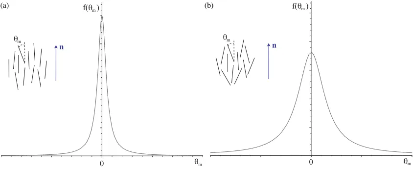
FIG. 2: (a) High orientational order: Ifθm denotes the angle between a molecule and the director and f(θm) is the
probability of finding a molecule with orientationθmin the small regionBthen for a highly ordered system,f(θm) has a
small standard deviation. (b)Low orientational order: We can still define the average orientation, i.e. the mean off(θm)
but in this case the molecules have more energy and the orientational distribution is more spread out. The standard deviation off(θm) is larger.
(discotic) molecules it will be the average orientation of the disc normal. If we consider a different region in the material the directornmay be in a different direction. This director may also vary with time and so it is a variable which is dependent on both space and time coordinates, n(x, t). We can also measure the amount of orientational order about this average direction, in the small ballB. If we consider all the molecules inB
and construct a probability distribution of the molecular orientations then the mean of this distribution is the director orientation but we can also compute, for instance, the standard deviation of the distribution. This would measure how spread out the molecular orientation distribution is. However, rather than the standard deviation of this distribution, the usual measure of this amount of order is thescalar order parameter, usually denoted byS. This is a weighted average of the molecular orientation angles θm between the long molecular
axes and the director
S= 1
2 <3 cos 2θ
m−1>, (1)
where<>denotes the thermal or statistical average so that
S=1 2
Z
B
(3 cos2θm−1)f(θm)dV, (2)
andf(θm) is the statistical distribution function of the molecular angle θm. Figure 2 shows typical statistical
distribution functions f(θm) for two cases, high orientational order and low orientational order. The function f(θm) will be even and periodic due to the head-tail symmetry of the molecules which impliesf(θm+π) =f(θm).
[image:2.612.89.511.229.402.2]x'
y'
z'
θ
m [image:3.612.229.373.78.205.2]φ
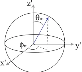
mFIG. 3: A description of the orientation of a single molecule in terms of the zenithal angleθmand azimuthal angleφm.
Thex0,y0andz0 axes are locally defined and are not the laboratory frame of reference.
sphere. The integration in eq. (2) may therefore be performed over half the boundary of the sphere, δB+ say in Fig. 1(b). An even function of θm must be used in eq. (1) because, since f(θm) is an even function, any
odd function of θm would lead to zero upon integration in eq. (2). To leading order this function is a good
approximate measure of the orientational order although a more accurate measure would include higher order polynomials of cosθm. Equation (1) is in fact the second order Legendre polynomial,P2(cosθm), and it is usual
to use the higher order even Legendre polynomialsP2n(cosθm) when greater accuracy is required.
When the material is crystalline all molecules align exactly with the director and soθm= 0 for all molecules,
which means that<cos2θ
m>= 1 and, from eq. (1),S= 1. When all molecules lie in the plane perpendicular
to the director, but randomly oriented in that plane, then the average still leads to the same director but
θm=π/2 for all molecules so that <cos2θm>= 0 andS =−1/2. In the isotropic liquid phase the molecules
are randomly oriented and sof(θm) is constant and equal to 1/(2π) (which can be derived from the property
of probability distributions thatR
f(θm)dV = 1). Therefore, performing the integration in eq. (2) in spherical
coordinates whereθmis the angle between the molecule and the director andφmis the azimuthal angle, i.e. the
angle between a fixed direction in the plane perpendicular to the director and the projection of the director onto that plane (see Fig. 3), we obtain (using the substitutionx= cos(θm) on the second line),
Z
δB+
cos2θmf(θm)dA =
1 2π
Z 2π
0
Z π/2
0
cos2θmsinθmdθmdφm
=
Z π/2
0
cos2θmsinθmdθm=−
Z 0
1
x2dx= 1
3 (3)
and so<cos2θm>= 1/3 and from eq. (1),S= 0.
Although it is possible to achieve a molecular configuration for whichS is negative, i.e. −1/2 < S < 0, it is more usual that in the equilibrium liquid crystal state the scalar order parameter is positive, 0< S <1. As the temperature of the material changes the scalar order parameter will change fromS = 0 in the isotropic state, at high temperature, toS = 1 in the crystalline state, at low temperature. A typical scalar order parameter in the middle of the phase region, for this type of liquid crystal, might beS = 0.6.
B. Biaxial nematics
The fundamental principle of any biaxial system is that there is no axis of complete rotational symmetry (i.e no axis about which a rotation ofany angle leaves the system unchanged), unlike a uniaxial system which has an axes of rotational symmetry (such as the director n in uniaxial liquid crystals). For instance, some solid materials (i.e. calcite) are uniaxial, and therefore birefringent, so that light travelling along the optical axis sees a different refractve index than light travelling perpendicular to the optic axis. However, other materials are biaxial (i.e. olivine), and have trirefringence, where there are three different refractive indices, for light travelling along three orthogonal directions.
In biaxial liquid crystals the two axes n and m are therefore defined and the symmetries are the reflections n→ −nandm→ −m.
The definition of three axes of reflective symmetry in a material is a relatively straightforward concept. Less straightforward is to understand the molecular arrangement corresponding to a biaxial systems. There are two possibilities for the shape of the molecules: either the molecules are uniaxial or they are biaxial. A uniaxial molecule can be thought of as shaped like a cylinder or rod (uniaxial because there is a rotation symmetry about the axis of the molecule), a biaxial molecule might be shaped like a plank of wood. There is no rotation axis along the long axis of the plank (rotating the plank changes its configuration) but there are three axes of reflective symmetry (the long, intermediate and short axis of the plank).
We can now have a uniaxial or biaxial arrangement of uniaxial molecules and a uniaxial or biaxial arrangement of biaxial molecules. The easiest arrangements to imagine are the uniaxial arrangement of uniaxial molecules - a group of cylindrical molecules oriented, on average, along a single direction where rotation about this direction does not alter, at least statistically speaking, the arrangement - and also the biaxial arrangement of biaxial molecules, a group of plank-shaped molecules where the long axes of the planks align in one direction and the short axes also align, in a second direction, so creating a biaxial ensemble arrangement.
A uniaxial arrangement of biaxial molecules is also relatively easy to imagine. In this arrangement the molecular long axes orient as before but the short axes of the plank are oriented randomly so that, if we view from the side as in Fig. 1, at any moment in time some of the planks are facing out of the page and some are turned end on. When you rotate the system the individual molecules look different but on average the same proportion of molecules are face on and end on (and all orientations in between).
A more difficult situation to imagine is a biaxial arrangement of uniaxial molecules. Such an alignment is described below and is the most relevant to the liquid crystal structure at the centre of defects.
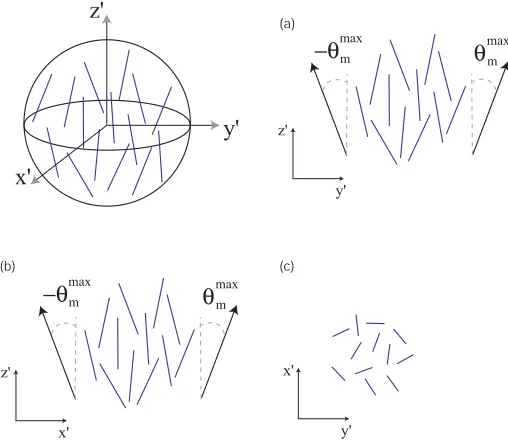
Imagine a group of uniaxial molecules (the cylindrical or rod-like molecules) which are in a uniaxial arrangement (Fig. 4) if you look down the director (the z0 axis) the molecules, which are now viewed almost end-on, look random, it is only the side view (along thex0ory0 axis) which indicates the directorn. Now restrict this group of molecules by “squashing” the distribution within the ball (see Fig. 5) between two imaginary plane surfaces parallel to the x0z0 plane, and look along the z0 axis again. There will be a restriction of the motion of the molecules in Fig. 4(c) to an arrangement similar to Fig. 5(c).
In more mathematical terminology: in the ballB, if the distribution of molecules is such that the zenithal angles
θmvary between−θmaxm andθ max
m and the azimuthal angles vary between−φ max m andφ
max
m then the three views
of the group of molecules along the x0, y0 and z0 axes are shown in Fig. 5(a), (b) and (c) respectively. If we look at the molecules along they0-axis (Fig. 5(b)) the extent of the zenithal angle is−θmax
m < θm< θmmaxand
we can define a scalar order parameterS1. If we look at the molecules along thez0-axis (Fig. 5(c)) the extent of the azimuthal angle is−φmax
m < φm< φmaxm and we can define a scalar order parameter S2 say. If we look along the x0-axis (Fig. 5(a)), the restriction to the azimuthal angle means we see an effective zenithal angle range which is smaller than in Fig. 5(a). Simple geometry gives us that theeffectiverange of zenithal angles is now
−θef fmax=−tan−1(sinφ max m tanθ
max
m )< θm<tan−1(sinφmaxm tanθ max m ) =θ
max
ef f (4)
Therefore, with this view, we would calculate a different scalar order parameter,S3say which is larger thanS1 (in factS3is related toS1andS2). It is now necessary to define three directors and corresponding scalar order parameters. If we take two perpendicular directorsnand m, in our situation thez0 andy0 directions, then we can define the two scalar order parametersS1andS2associated with order about the two directors respectively (the third director beingn×m). If the order parameter S2 is non-zero and not equal to S1 the liquid crystal is said to be biaxial, i.e. there are two axes of symmetry. If, however, S2=0 then in comparison to Fig. 5(c) the range of azimuthal angles is now−π/2< φm< π/2 and a view along thez0-axis shows randomly oriented
molecules (see Fig. 4). The view from thex0-axis will show a regular nematic distribution of molecules and the director and a non-zero order parameter S1 can be defined. Since the system of molecules is now rotationally symmetric about thez0-axis, the view along they0 axis will be the same as that along thex0-axis and thus the order parameter will again beS1.
From these examples we see that the uniaxial nematic state exists when the order parameter with respect to one direction is zero, or equivalently the order parameters with respect to the perpendicular directions are the same. The biaxial nematic state exists when the scalar order parameters in all three perpendicular directions are different.
m
−θ
maxθ
mmax (b)
x' z'
(a)
y' z'
(c)
y' x'
m
−θ
maxθ
mmax
x'
[image:5.612.173.427.76.300.2]y'
z'
FIG. 4: A uniaxial distribution of molecules. Viewed along thex0ory0-axes the molecular distribution is similar and the
calculated scalar order parameter is identical. Viewed along the director, thez0-axis, the molecules are viewed virtually
end-on and the distribution looks isotropic.
m
−θmax θmmax
(b)
x' z'
eff
−θmax θeff
max (a)
y' z'
m
−φmax φm
max (c)
y' x'
x'
y' z'
FIG. 5: A biaxial distribution of molecules. Viewed along the three local axes the scalar order parameter, i.e. how spread out the molecules are, is different in each case
(after over 50 years of searching). Many attempts to synthesise such a material, mainly using flat, board-like molecules, have failed and it seems that bent-core molecules have provided the solution [3–5]. The biaxial state is certainly important since certain external forces such as surfaces in contact with the liquid crystal, electric fields and some topological constraints can induce a biaxial state in regions of a uniaxial nematic liquid crystal sample.
In this paper we will only consider an ensemble of rod-like (i.e. uniaxial) molecules which, as mentioned above, may form a uniaxial or biaxial configuration. Consideration of an ensemble of plank-like or bent core (i.e. biaxial) molecules is more complicated and involves a second order tensor B to describe the ordering of the short molecular axes. Such a theory is detailed in Sonnet and Virga [2].
[image:5.612.171.428.363.554.2]x
y
z
θ
φ
n
m
[image:6.612.244.357.78.173.2]ψ
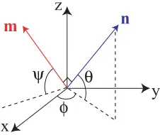
FIG. 6: The directorsnandmin terms of the Euler anglesθ,φandψ. The axesx,yandz form the laboratory frame
of reference.
S1(x, t) andS2(x, t), all of which may depend on the spatial coordinatesxand time.
We assume, without loss of generality, that the directors are of unit length, |n|= 1 and|m|= 1. Just as we have described each molecule in Fig. 3, each of these directors can be represented in terms of the standard Euler angles, see Fig. 6. Since the directornis of unit length it can be written as,
n= (cosθcosφ, cosθsinφ, sinθ). (5)
It is important not to confuse the director anglesθ andφ with the molecular angles in Fig. 3. The molecular anglesθm andφmare angles relative to a local frame of reference, i.e. the directors, whereas the angles θand φare defined relative to the laboratory frame of reference, i.e a set of axes fixed in space, independent of the orientation of the material.
The directormis perpendicular tonand therefore has one remaining degree of freedom, the angleψ,
m= (sinφcosψ−cosφsinψsinθ, −sinφsinψsinθ−cosφcosψ, sinψcosθ). (6)
The angleψis the angle frommto the direction (sinφ, −cosφ, 0) in thexy-plane which is also perpendicular ton.
A theory can now be constructed using thefivedependent variables,
θ(x, t), φ(x, t), ψ(x, t), S1(x, t), S2(x, t). (7)
However, there may be problems with a theory such as this, based on Euler angles. When the zenithal angle
θ equals π/2 the azimuthal angle φ is undefined and, as with all such angle variables, there may also be a problem with multi-valuedness sinceφ= 0 is equivalent toφ= 2π. Care must be taken when solving governing differential equations forθ,φandψ.
C. The tensor order parameter Q
We now define an alternative approach which removes the problems of the angle representation described above. Instead of defining the nematic state in terms of the five separate variables in eq. (7) we construct a 3x3 matrix which contains all the information about the nematic state, i.e. the information contained in the five variables. The problems of solving the Euler angle governing equations will be removed with this approach (for reference see for example [1, 2]).
Consider the 3x3 matrix,
M=S1(n⊗n) +S2(m⊗m), (8)
where, for any vectorhtheijth element of the producth⊗hishihj, theith element ofhmultiplied by the jth element ofh. This matrix will be symmetric, sincen
inj =njni and mimj =mjmi, and the trace ofM
will beS1(n1n1+n2n2+n3n3) +S2(m1m1+m2m2+m3m3) =S1+S2 since|n|= 1 and|m|= 1
Since the trace ofMis fixed and the matrix is symmetric,Mwill have five independent elements,
M=
m1 m2 m3
m2 m4 m5
m3 m5 (S1+S2)−m1−m4
The tensorMcontains the same information as the five separate variables in eq. (7). However, if we construct a theory usingM there will be no problems with the degeneracies of Euler angles.
As will be indicated later, it is actually more useful to use the tensor,
Q=S1(n⊗n) +S2(m⊗m)− 1
3(S1+S2)I, (10)
where I is the identity matrix so that the trace of Q is zero. The tensor order parameter Q is therefore a symmetric traceless matrix and can be written as,
Q=
q1 q2 q3
q2 q4 q5
q3 q5 −q1−q4
, (11)
and from the definitions ofnandmand eqs (10) and (11) we see that the elementsqi can be written in terms
of the variablesθ,φ,ψ,S1andS2thus,
q1 = S1cos2θcos2φ+S2(sinφcosψ−cosφsinψsinθ) 2
−1
3(S1+S2), (12)
q2 = S1cos2θsinφcosφ
−S2(cosφcosψ+ sinφsinψsinθ) (sinφcosψ−cosφsinψsinθ), (13)
q3 = S1sinθcosθcosφ+S2sinψcosθ(sinφcosψ−cosφsinψsinθ), (14)
q4 = S1cos2θsin2φ+S2(cosφcosψ+ sinφsinψsinθ) 2
−1
3(S1+S2), (15)
q5 = S1cosθsinθsinφ−S2sinψcosθ(cosφcosψ+ sinφsinψsinθ). (16)
From the previous section, the description of biaxiality tells us that, if the matrixQwas diagonalised (so that the eigenvectors are along thex0,y0andz0 directions) then for a uniaxial state two of the eigenvalues would be the same and for a biaxial state all three eigenvalues would be different.
The eigenvalues of the matrixQ, described by eqs (12)-(16), are,
λ1 = (2S1−S2)/3, (17)
λ2 = −(S1+S2)/3, (18)
λ3 = (2S2−S1)/3. (19)
Uniaxial states exist when two of these eigenvalues are the same i.e. when λ1 = λ2 so that S1 = 0 or when
λ2 =λ3 so S2 = 0 or whenλ1 =λ3 so S1 =S2. When all the eigenvalues are the same we have an isotropic system and we have S1 = 0 and S2 = 0 so that Q=0. We shall see later that the use ofQ rather thanM as our dependent tensor variable was in fact dictated by the property that the isotropic state is described by Q=0.
If we, for simplicity, define our laboratory axes to be such that the directorsnand m are in the directions of thexandy axes thenθ= 0, φ= 0 andψ=πso that
q1 = 1
3(2S1−S2), (20)
q2 = 0, (21)
q3 = 0, (22)
q4 = 1
3(2S2−S1), (23)
q5 = 0, (24)
and therefore the three possible uniaxial states correspond to: q1 = −q1−q4 so that q1 = −q4/2 = −S2/3;
−q1−q4=q4 so thatq4=−q1/2 =−S1/3; orq1=q4=S1/3 =S2/3.
II. PHENOMENOLOGICAL THEORY
In order to form a theoretical framework to consider such liquid crystals it is necessary to construct the total free energyFof the liquid crystal sample, which may include terms such as: the elastic energy of any distortion to the structure of the material; thermotropic energy which dictates the preferred phase of the material; electric and/or magnetic energy from an externally applied electric or magnetic field and, in polar materials, the internal self-interaction energy of the polar molecules; surface energy terms representing the interaction energy between the bounding surface and the liquid crystal molecules at the surface. The total energy is therefore,
F = Fdistortion+Fthermotropic+Felectromagnetic+Fsurf ace
=
Z
V
(Fd+Ft+Fe) dv+
Z
S
(Fs) ds, (25)
where the energy densities,Fd, Ftetc., depend on the dependent variables, the tensor order parameter elements.
In static situations minimisation of this energy, using the calculus of variations, leads to sets of differential equations in the bulk of the material and at the surface, for each of the dependent variables. The solution of these bulk equations subject to the surface boundary conditions gives the equilibrium configuration of the dependent variables through the sample.
The free energy density is assumed to depend on the tensor order parameterQand all first order differentials ofQ. It is also assumed that distortions ofQare small and therefore higher order differentials and high powers of first order differentials will be negligible. The bulk free energy density,Fb=Fd+Ft+Fe, will be an integral
of a function dependent on the elements ofQand all derivatives of the elements whereas the surface free energy density is assumed to be a function of the elements ofQonly,
F=
Z
V
Fb(qi,∇qi) dv+
Z
S
Fs(qi) ds. (26)
Static equations
The governing differential equations forqi(x) are the Euler-Lagrange equations, the solution of which minimises
the free energy. The general Euler-Lagrange equations for the free energy eq. (26) are the five equations
3
X
j=1
∂ ∂xj
∂F
b ∂qi,j
= ∂Fb
∂qi
, (27)
fori= 1. . .5 and whereqi,j=∂qi/∂xj. These five equations should be solved together with suitable boundary
conditions.
Equations (27) may be written as
∇.ΓΓΓi=fi, (28)
where
Γij = ∂Fb
∂qi,j
, (29)
fi = ∂Fb
∂qi
. (30)
Dynamic equations
When the dynamic evolution of the Qtensor is required and the coupling between the director rotations and fluid flow is thought to be small (an assumption that is not always true, but see [2] for a full dynamical theory), a dissipation principle can be used to show that the governing equations will be,
γ∂D ∂q˙i
=∇.ΓΓΓi−fi, (31)
whereDis the dissipation function
D= tr
∂Q
∂t
2!
˙
qi =∂q/∂xi and the viscosity γ is related to the standard nematic viscosity γ1 (which is equal to α3−α2 in Leslie viscosities) by,
γ= γ1
Sexp
, (33)
whereSexpis the uniaxial order parameter of the liquid crystal when the experimental measurement ofγ1 was taken.
Boundary conditions
Two types of boundary conditions will be considered; strong (infinite) or weak anchoring.
(i) Strong: For strong, also termed infinite, anchoring we use Dirichlet conditions. That is, the order tensor will be fixed at a specified value at the domain boundary that has been dictated by some substrate alignment technique. In this case the boundary condition is
Q=Qs, (34)
whereQsis the prescribed order tensor at the boundary. In this case there is no surface energy and Fs= 0 in
eq. 25.
(ii)Weak: For a weak anchoring effect there exists a surface energy,Fs, which is added to the free energy and
must be minimised at the same time as the bulk free energy. This minimisation leads to the condition that, on the boundary, the liquid crystal variablesqi satisfy
X
j=1,2,3
νj
∂F
b ∂qi,j
= ∂Fs
∂qi
(35)
or equivalently
ν ν
ν.ΓΓΓi=Gi (36)
where ΓΓΓi is as in eq. (29), Gi =−∂F
s/∂qi and whereννν is the normal to the substrate. Usually the surface is
planar or circular so that the surface normal is relatively simple, for exampleννν = (0,0,1) if the surface is a plane parallel to thexy-plane. However, in general the substrate normal is position dependentννν(x).
In order to complete this theory it is necessary to specify each of the components of the free energy. The following sections describe the thermotropic, elastic, electrostatic and surface energies.
A. Landau-de Gennes thermotropic energy
The thermotropic energy,Ft, is a potential function which dictates which state the liquid crystal would prefer
to be in, i.e. a uniaxial state, a biaxial state or the isotropic state. At high temperature this potential should have a minimum energy in the isotropic state, i.e.Q=0whereas at low temperatures there should be minima at three uniaxial states, i.e. the states where any two of the eigenvalues ofQare equal. For rod-like molecules a bulk biaxial minimum energy state is not possible[2]. The simplest form of such a function is a truncated Taylor expansion aboutQ=0[6],
Ft=atr Q2
+2b 3 tr Q
3
+c 2 tr Q
22
(37)
which is a quartic function of theqis. This energy is sometimes written as
Ft=atr Q2
+2b 3 tr Q
3
+ctr Q4
. (38)
Equations (37) and (38) are equivalent only if the factor of two in thec term is included. This form of energy can also be thought of as an expansion in terms of the two invariants of the order tensor, tr Q2and det(Q).
The coefficientsa, b and c will in general be temperature dependent although it is usual to approximate this dependency by assuming that b and c are independent of temperature whilst a= α(T−T∗) = α∆T where
As stated in Section I C, the eigenvalues ofQareλ1= (2S1−S2)/3, λ2=−(S1+S2)/3, λ3= (2S2−S1)/3 and since the trace of the nth power of Qis the sum of the nth powers of these eigenvalues, thus the thermotropic energy is simply a function ofS1andS2,
Ft = a
3
X
i=1
λ2i +2b 3
3
X
i=1
λ3i + c 2
3
X
i=1
λ2i
!2
(39)
= 2a
3 S
2
1−S1S2+S22
+2b 27 2S
3
1−3S21S2−3S1S22+ 2S23
(40)
+2c
9 S
4 1−2S
3
1S2+ 3S12S 2
2−2S1S23+S 4 2
For a uniaxial state such asλ2=λ3, or equivalently S2= 0, the thermotropic energy becomes,
Ft =
2 27 9aS
2 1+ 2bS
3 1+ 3cS
4 1
(41)
Which has stationary points whendFt/dS1= 0 so that,
S1 = 0 (42)
S1 = 1 4c
−b+pb2−24ac (43)
S1 = 1 4c
−b−pb2−24ac (44)
This calculation can be performed using the qi variables if we first assume for simplicity that the laboratory
frame of reference is set such that the directors are along the axes, as in Section I B. In this case we obtain the stationary points of the free energy as,
q1 = 0 (45)
q1 = 1 6c
−b+pb2−24ac (46)
q1 = 1 6c
−b−pb2−24ac (47)
By calculatingd2F
t/dS21 and comparing the energies of each solution we find that
• S1 = 0, the isotropic state, is globally stable fora > b 2
27c, metastable for 0< a < b2
27c and unstable for a <0.
• S1= 41c −b+
√
b2−24ac
, the nematic state, is globally stable fora < 27b2c, metastable for 27b2c < a < 24b2c
and not defined fora > 24b2c.
• S1= 41c −b−
√
b2−24ac
is metastable (but has a negative value) fora <0, unstable for 27b2c < a < 24b2c
and not defined fora > 24b2c.
The equilibrium nematic scalar order parameter (43) will be denoted bySeq.
There are clearly three important values ofa: a= 24b2c, the high temperature where the nematic state disappears;
a= 27b2c, the temperature at which the energy of the isotropic and nematic states are exactly equal;a= 0, the low temperature where the isotropic state loses stability. If we use the notationa=α(T−T∗) then the critical temperatures areT+=24b2αc+T∗;TN I= b
2 27αc+T
∗;T =T∗.
–0.4 –0.2 0 0.2 0.4 0.6 q 1 –0.4 –0.2 0 0.2 0.4 0.6 q 4 0 2000 4000 6000 8000 10000 –0.4 –0.2 0 0.2 0.4 0.6 q1 –0.4 –0.2 0 0.2 0.4 0.6 q4 0 2000 4000 6000 8000 10000 –0.4 –0.2 0 0.2 0.4 0.6 q 1 –0.4 –0.2 0 0.2 0.4 0.6 q 4 0 2000 4000 6000 8000 10000 –0.6 –0.4 –0.2 0 0.2 0.4 0.6 0.8 q 1 –0.6 –0.4 –0.2 0 0.2 0.4 0.6 0.8 q 4 –8000 –6000 –4000 –2000 0 2000 4000 6000 8000 10000 –0.6 –0.4 –0.2 0 0.2 0.4 0.6 0.8 q 1 –0.6 –0.4 –0.2 0 0.2 0.4 0.6 0.8 q 4 –20000 –15000 –10000 –5000 0 5000 10000 –0.6 –0.4 –0.2 0 0.2 0.4 0.6 0.8 q 1 –0.6 –0.4 –0.2 0 0.2 0.4 0.6 0.8 q 4 –20000 –15000 –10000 –5000 0 5000 10000 F t (a) (b) (c) (e) (f) (d)
FIG. 7: The thermotropic potential for parametersα= 0.042×10⁶Nm−2K−1,b=−0.64×10⁶Nm−2,c= 0.35×10⁶Nm−2 [7] and (a) ∆T = 2.0, (b) ∆T = 1.5, (c) ∆T = 1.0, (d) ∆T = 0.5, (e) ∆T = 0.0, (f) ∆T =−0.1. At high temperatures (a,b) only the isotropic state is stable and at low temperature (d,e,f) the three uniaxial states are stable. At intermediate temperatures (c) both the isotropic and all three nematic states are stable.
8. In these figures the tensor order parameter is assumed to be diagonalised so that the directors align with the laboratory frame of reference. Therefore, as mentioned in Section I C, the off diagonal terms ofQare zero and
Ftdepends only onq1andq4. Figure 7(a) clearly shows the three uniaxial states and as temperature increases the potential function changes to exhibit a single minima at the isotropic state.
–20000 –10000 0 10000 20000 30000
–0.2 0 0.2 0.4 0.6 0.8
q1 Ft
ΔT=0.5
ΔT=0.0
ΔT=0.5
ΔT=-0.1
ΔT=1.0
[image:12.612.172.429.73.397.2]ΔT=2.0
FIG. 8: Cross-section of Fig. 7 along the line q4 = q1/2, the equivalent to the uniaxial state S2 = 0, for varying
temperature with the parameter valuesα= 0.042×10⁶Nm−2K−1,b=−0.64×10⁶Nm−2,c= 0.35×10⁶Nm−2 [7]. At
∆T = 0.5 both the isotropic minima (q1= 0) and the uniaxial nematic minima (q16= 0) are locally stable.
assume that higher order powers ofQ may be neglected in eq. (37). The first five powers of Q are included in eq. (37) (the constant term is neglected as it will not enter into a minimisation of the energy and the linear term is taken to have zero coefficient since tr(Q) = 0 so that there is a minimum at Q= 0) since we assume there are at most four minima in the potential functionFt.
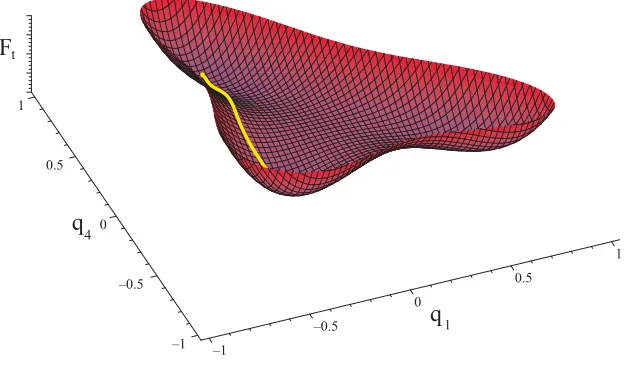
It would be energetically favourable for the system to lie in one of the minima ofFt. When a liquid crystal
material is forced to contain some form of distortion (e.g. through the influence of surface or electric field effects) there are two mechanisms for undertaking such a distortion. For example imagine a region of liquid crystal constrained to lie between two solid surfaces. If, through some surface treatment, one of the surfaces forces the liquid crystal in contact with that surface to lie in a fixed uniaxial state, i.e in one of the minima of Fig. 7(a) whereas the other surface forces the liquid crystal in contact with it to lie in a different uniaxial state. Firstly, for the system to move from one minima ofFt to another, the eigenvectors ofQ may change. This is
equivalent to the molecular frame of reference changing. The system effectively rotates the picture in Fig. 7 so that the system always remains in the same minima ofFt, it is simply that the minima itself that changes
–1
–0.5
0
0.5
1
q
–1 –0.5 0 0.5 1
1 4
q
t
[image:13.612.145.458.74.257.2]F
FIG. 9: A schematic plot of how a system may be forced out of the thermotropic potential minimum. At one point in the liquid crystal (represented by one end point of the yellow line) the system is forced, through some external agent, to lie at one of the uniaxial states. At another point in the liquid crystal (represented by the other end point of the yellow line) the system is forced to lie in a different uniaxial states. For the macroscopic variables to be continuous through the region the system continuously transforms from one state to the other, at some points moving out of the potential minima. The yellow line plots the state variables on the potential energy surface of the system from one region in the liquid crystal to the other.
B. Elastic energy
The distortional or elastic energy density,Fd, of a liquid crystal is derived from the energy induced by distorting
theQ tensor in space. It is, generally, energetically favourable forQ to be constant throughout the material and any gradients in Qwould lead to an increase in distortional energy. Fd therefore depends on the spatial
derivatives ofQ. Given a fixed distortion in space of Q the distortional energy must remain unchanged if we were to translate or rotate the material. Such restrictions (or symmetries) mean that not all combinations of Qderivatives are allowed. In fact the elastic energy may be simplified to [8],
Fd =
X
i=1,2,3 j=1,2,3 k=1,2,3
"
L1 2
∂Q
ij ∂xk
2
+L2 2
∂Qij ∂xj
∂Qik ∂xk
+L3 2
∂Qik ∂xj
∂Qij ∂xk
#
+ X
i=1,2,3 j=1,2,3 k=1,2,3 l=1,2,3
L
4 2 elikQlj
∂Qij ∂xk
+L6 2 Qlk
∂Qij ∂xl
∂Qij ∂xk
. (48)
The coordinates (x1, x2, x3) = (x, y, z) are the usual Cartesian coordinate system andQij is theijthelement
The elastic parametersLi are related to the Frank elastic constantskij by [8]
L1 = 1 6S2
exp
(k33−k11+ 3k22), (49)
L2 = 1
S2
exp
(k11−k22−k24), (50)
L3 = 1
S2
exp
k24, (51)
L4 = 2
S2
exp
q0k22, (52)
L6 = 1 2S3
exp
(k33−k11), (53)
where Sexp is the uniaxial order parameter of the liquid crystal when the experimental measurement of the Li was taken and may not be equal to the current order parameterSeq = −b+
√
b2−24ac
/(4c) mentioned in Section II A. The parameterq0 is the chirality of the liquid crystal and if an achiral liquid crystal is under consideration thenL4= 0.
It has been shown that there are seven elastic terms of cubic order [9, 10] but we will only include one, theL6 term in eq. (48), in order to ensure we can model a nematic state with non-equal elastic constantsk11,k22,k33. Without theL6term we have four elastic parametersL1, . . . , L4in theQtensor elastic energy but we have five independent parameters in the Frank approach,k11,k22, k33, k24 and q0. Including theL6 term removes the degeneracy in the mapping from theQtensor to the Frank energy approaches.
C. Electrostatic energy
The liquid crystal will interact with an externally applied electric field or indeed self-induce an internal electric field due to the dielectric and spontaneous polarisation effects. The electrostatic energy density is
Fe=−
Z
D.dE, (54)
whereDis the displacement field andEis the electric field. The constitutive equation,
D = 0E+P
= 0E+Pi+Ps
= 0E+0χχχE+Ps
= 0E+Ps, (55)
relates the displacement field with the electric fieldEand the internal polarisationP. This polarisation is split into dielectrically induced polarisation Pi and the spontaneous polarisation Ps. The induced polarisation is
dependent on the dielectric susceptibilityχand the electric field Eand the dielectric tensor is then defined as
=I+χwhereIis the identity matrix. The electrostatic energy density is then,
Fe=−
Z
(0E+Ps).dE=−
1
20(E).E−Ps.E. (56)
In a nematic liquid crystal the dielectric tensor is approximated to= ∆∗Q+ ¯Iwhere ∆∗= (||−⊥)/Sexp
is the scaled dielectric anisotropy and ¯= (||+ 2⊥)/3 is an average permittivity. Within an isotropic material, such as an alignment layer of photo-resist material, the dielectric tensor is diagonal and isotropic,=II.
In the present, nematic, situation a spontaneous polarisation vector is assumed to derive only from a flexoelectric type of polarisation, that is a polarisation caused by a distortion of the molecular arrangement. This may be due to a shape asymmetry in the molecules or due to a distortion of a pair-wise coupling of molecules. For either of these mechanisms, the polarisation may be written, to leading order, in terms of theQtensor as [11],
where theith component of∇.Qis understood to beP
j=1,2,3∂Qij/∂xj.
If we consider the flexoelectric polarisation of a uniaxial state, whereQ=S((n⊗n)−I/3), we find
Ps= ¯e
S(∇.n)n+S(∇ ×n)×n+ (n.∇S)n−1
3∇S
. (58)
Comparing this to the standard expressions for flexoelectric polarisation and order electricity [12–14],
Pf = e11(∇.n)n+e33(∇ ×n)×n, (59)
Po = r1(n.∇S)n+r2∇S, (60)
we see that eq. (57) is equivalent to eqs (59) and (60) when we set e11 = e33 = Se¯ and r1 = ¯e, r2 =
−e/¯ 3. Therefore, without taking higher order terms in eq. (57), this expression assumes that the coefficients of flexoelectric and order electric terms are equal. Within a region where S is constant, only the flexoelectric polarisation eq. (59) would be present.
In order to distinguish between the flexoelectric parameterse11 ande33 higher order terms are needed in the flexoelectric polarisation term in eq. (57) [15]. For instance, if we include second order terms theithcomponent of the polarisation vector is
(Ps)i=p1
X
j=1,2,3
∂Qij ∂xj
+p2
X
j=1,2,3 k=1,2,3
Qij ∂Qjk
∂xk
+p3
∂ ∂xi
X
j=1,2,3 k=1,2,3
QjkQjk
+p4
X
j=1,2,3 k=1,2,3
Qjk ∂Qji
∂xk
. (61)
For a uniaxial material we can substitute, expand and collect terms as before. This gives
e11 = Sp1+
S2
3 (2p2−p4),
e33 = Sp1+
S2
3 (2p4−p2),
r1 = p1+
S
3(p2+p4),
r2 = 1 3
−p1+
S
3(p2+p4) + 4Sp3
.
Therefore, including second order terms does allow us to have different values fore11ande33ifp26=p4. However, deciding on values forp1. . . p4is non-trivial. Barbero et al. [14] have stated thatp1,p2andp4can be obtained by measuring the flexoelectric parameters as a function of temperature, and assume a similar magnitude forp3, but there seems to be no such measurements in the literature.
At this point the electric field within the whole cell is unknown but may be found using Maxwell’s equations which are, in this static case with no free charges,
∇.D = 0, (62)
∇ ×E = 0. (63)
Equation (63) means that we may define a scalar functionU, the electric potential, which satisfiesE=−∇U
(it is convention to makeEthe negative gradient ofU). If we find the functionU then eq. (63) is automatically satisfied. Equation (62) is then the governing equation for the electric potentialU,
0 = ∇.D=∇.(−0∇U+Ps), (64)
and the free energy density,
Fe=−
1
20∇U.∇U+Ps.∇U, (65)
will enter the total free energy density to be minimised in order to obtain the Euler-Lagrange equations for the
qi. Equation (64) is in fact equivalent to the Euler-Lagrange equation derived from minimising the free energy
in eq. (65) with respect toU.
D. Surface energy
When the liquid crystal molecules are close to a solid surface they will feel a molecular interaction force. Whatever this force is we would like to model this liquid crystal-surface interaction in a macroscopic framework. That is, how does the surface interact with the macroscopic variables (the elements of the tensor order parameter Q). If the surface is treated is some way, usually by coating the surface with a chemical and possibly rubbing the surface in a fixed direction so as to create a preferred surface direction, then we will assume that at that surface the directorsn and m would prefer to lie in a certain direction. We may also assume that the solid surface may affect the amount of order (i.e. the variables S1 and S2) at that surface. Associated with this preference for a certain orientation and order will be asurface energy, Fsurf ace, which will have a minimum
at the preferred state. This surface energy will be a function of the value of the dependent variables at the surface. Thus, ifS is the surface in contact with the liquid crystal, Fsurf ace=Fsurf ace(Q|S). If the variables are forced to move out of the minima, usually by the bulk of the liquid crystal being in some alternate state, then the surface energy will increase and there will be a competition between surface energy and bulk energy. In equilibrium, a balance will be reached such that the total energy in eq. (25) is minimised.
Weak anchoring: One simple form of the free energy density,Fs, has a single minimum at the point where
the dependent variables take the value dictated by the surface treatment,
Fs= W
2 tr (Q|S−Qs) 2
(66)
where Qs is the value of the tensor order parameter preferred by the surface and W is the anchoring energy.
When the system is in equilibrium the calculus of variations gives the set of boundary conditions in eqs (35) which are similar to a torque balance at the surface, of the distortion torque and the torque due to the surface energy function. If we were to compare this energy to a Rapini-Papoular type anchoring energy where, say, a preference for the director to lie in the xdirection is given by the energy density Fs = W2ssin2θ, then the
relationship between the Rapini-Papoular anchoring strengthWsand theQtensor anchoring strength in eq. (66)
will be,
W = Ws 2Ss2
, (67)
whereSsis the preferred surface order parameter.
An example of the type of anchoring in eq. (66) is if we have a surface which prefers the nematic to be uniaxial with the director in the z direction and scalar order parameter of 0.6. We then take S2 = 0, θ = π/2 and
S1= 0.6 in eqs (12-16) so that the preferredQtensor is,
Qs=
−0.2 0 0 0 −0.2 0 0 0 0.4
, (68)
or in terms of theqi values,q1=−0.2, q2= 0.0, q3= 0.0, q4=−0.2, q5= 0.0.
Another important example of weak anchoring is homeotropic anchoring on a non-planar surface. Such anchoring prefers the director to lie perpendicular to the surface at all points. If we denote the unit normal to the surface asννν = (νx, νy, νz) then this will be the preferred director. If we assume that the surface will prefer a uniaxial
state (as suggested by the local symmetry of homeotropic anchoring) then we may use eq. (10) with n =ννν,
S1=SsandS2= 0 to obtain the preferred Qtensor,
Qs=Ss
νx2−13 νxνy νxνz νxνy νy2−13 νyνz νxνz νyνz 32−νx2−νy2
. (69)
Strong/infinite anchoring: The case of strong anchoring mentioned in Section II is equivalent to the limit
Ws→ ∞, and is therefore often termed infinite anchoring. In this case the Dirichlet condition
Q=Qs, (70)
Planar degenerate anchoring: Another common liquid crystal substrate (i.e. untreated SU8) leads to planar degenerate anchoring. In this situation the preferred orientation for the directors is to lie parallel to the substrate. There is no preference as to which direction on the plane of the surface to lie but simply that the director lies on the surface.
The most general surface energy density in this case is [16],
Fs = c1ννν.Q.ννν+c2(νν.νQ.ννν)2+c3ννν.Q2.ννν
+astr Q2
+2bs 3 tr Q
3
+cs 2 tr Q
22
. (71)
In this energy density the first three terms give the most general energy density, up to quadratic order, which specifies that the eigenvectors of Qlie parallel to the surface with normalννν. The last three terms in eq. (71) are added to specify preferred eigenvalues ofQ.
If we assume the liquid crystal has taken a uniaxial state at the surface,S1 =S and S2 = 0, then the planar degenerate surface energy density is
Fs= S
3 3c2Ssin
4θ+ (3c
1+ (c3−2c2)S) sin2θ
+f(S), (72)
which has a minimum atθ= 0 whenS(3c1+ (c3−2c2)S)>0. The effective anchoring strength, when compared to a Rapini-Papoular energy, may be thought of as Ws = 23S(3c1+ (c3−2c2)S). It is clear that there is no dependence on the azimuthal angleφas such a degenerate anchoring condition would suggest.
With all terms in the free energy now specified, as well as appropriate examples of boundary conditions, it is possible to apply the governing equations to a realistic problem.
III. EXAMPLE: THE ZENITHAL BISTABLE DEVICE
x z
electrode, U=V
electrode, U=0
alignment layer
photo-resist liquid crystal
[image:17.612.200.402.423.641.2]3µm
FIG. 10: Typical ZBD cell. A periodic grating structure formed out of a photo-resist material. The upper surface is coated with an alignment layer material and electrodes are placed around the system. In the numerical computation we assume that we may consider only one of the repeating cells and enforce periodic boundary conditions.
-0.2 -0.1 0 0.1 0.2 0.3 0.4
-0.15 -0.1 -0.05 0 0.05 0.1 0.15 0.2 0.25 0.3
-0.23 -0.22 -0.21 -0.2 -0.19 -0.18 -0.17
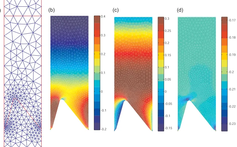
[image:18.612.111.501.78.320.2](a) (b) (c) (d)
FIG. 11: ZBD display with zero voltage, the HAN state: (a) finite element mesh and the solutions for (b)q1, (c)q2, (d)
q4.
photoresist surface we will assume that there exists homeotropic anchoring so that the preferred Q tensor is a uniaxial tensor with a director in the surface normal direction. We therefore use the boundary condition in eq. (35) and the surface energy in eq. (66) with eq. (69).
The electric potentialU will be solved within the whole region bounded by the two electrodes. Within the whole regionU is subject to eq. (64) where the dielectric tensor is different within the alignment layer, the liquid crystal layer and the photo-resist. Within the alignment layer =aI, in the liquid crystal layer = ∆∗Q+ ¯Iand
within the photo-resist=pI. The boundary conditions for U areU = 0 at the bottom electrode andU =V
at the top electrodes.
We will also apply periodic boundary conditions on twoyz planes (dashed lines in Fig. 10) in order to model an infinite periodic grating. In this example no voltage is applied to the electrodes.
Using MATLAB[19] and the finite element modelling package COMSOL[20] the domain is meshed (see Fig. 11(a)) and the solution of the governing equations is found. As an example Figure 11 shows the solu-tions for q1, q3 and q4. The variables q2, q5 and U are identically zero through the region. Possibly more instructive are plots of the eigenvalues and eigenvectors ofQ, see Figure 12.
From Fig. 12 we see that there exist two regions where the eigenvalues vary significantly. Near the peak and trough of the grating structure there exist -1/2 and +1/2 defects respectively. This defect structure means that in the region immediately above the grating the director (the eigenvector in Fig. 12(d)) is almost horizontal and a hybrid aligned nematic (HAN) type structure results.
IV. SUMMARY
In this paper we have introduced a simple form of theQ-tensor theory for calamitic nematic liquid crystals. We have described the governing equations for a model where fluid flow is neglected and given the forms for the constitutive components of energy and dissipation. This paper should hopefully allow both simple numerical models of liquid crystal devices to be constructed and give the reader a better understanding of the vast array of publications written in the last 10-15 years which have utilised such a theory.
-0.23 -0.22 -0.21 -0.2 -0.19 -0.18 -0.17
-0.2 -0.15 -0.1 -0.05 0 0.05
0.15 0.2 0.25 0.3 0.35 0.4
[image:19.612.105.503.73.288.2](a) (b) (c) (d)
FIG. 12: ZBD display with zero voltage, the HAN state: the three eigenvalues (a), (b) and (c) and the eigenvector associated with the largest eigenvalue.
scale of 10s or 100s of microns) and the defect core (on the scale of 10s to 100s of nanometres) means that discretisation of even a static example can lead to large numbers of numerical elements. A non-uniform grid is essential and, if the dynamic equations are to be solved, both adative meshing and timestepping will also be necessary. A number of papers have been written about these topics and those attempting to model such systems would be advised to consult these papers or seek assistance from researchers in the area[21–23].
[1] E. G. Virga,Variational theories for liquid crystals, Chapman & Hall, London (1994).
[2] A. M. Sonnet and E. G. Virga,Dissipative Ordered Fluids: Theories for Liquid Crystals, Springerl, New York (2010).
[3] L. A. Madsen, T. J. Dingemans, M. Nakata, and E. T. Samulski,Thermotropic biaxial nematic liquid crystals, Phys.
Rev. Lett.92, 145505 (2004).
[4] B. R. Acharya, A. Primak, and S. Kumar,Biaxial nematic phase in bent-core thermotropic mesogens, Phys. Rev.
Lett.92, 145506 (2004).
[5] G. R. Luckhurst, S. Naemura, T. J. Sluckin, S. K. Thomas, & S. S. Turzi, Molecular-field-theory approach to the
Landau theory of liquid crystals: Uniaxial and biaxial nematics, Phys. Rev. E85, 031705 (2012).
[6] N. Schophol and T. J. Sluckin,Defect core structure in nematic liquid crystals, Physical Review Letters59, p.2582
(1987).
[7] E. B. Priestley, P. J. Wojtowicz and P. Sheng,Introduction to liquid crystals, Plenum Press, New York and London
(1976).
[8] H. Mori, E. C. Gartland, J. R. Kelly and P. J. Bos,Multidimensional director modeling using the Q tensor
repre-sentation in a liquid crystal cell and its application to the π cell with patterned electrodes, Jap. J. App. Phys. 38, p.135 (1999).
[9] D. W. Berreman and S. Meiboom,Tensor representation of Oseen-Frank strain energy in uniaxial cholesterics, Phys.
Rev. A30, p.1955 (1984).
[10] K. Schiele and S. Trimper,On the elastic constants of a nematic liquid crystal, Physica Status Solidi B118, p.267
(1983).
[11] A. L. Alexe-Ionescu, Flexoelectric polarisation and 2nd order elasticity for nematic liquid crystals, Phys. Lett. A
180(6), p.456 (1993).
[12] R. Meyer,Piezoelectric effects in liquid crystals, Phys. Rev. Lett.22, p.918 (1969).
[13] P. G. de Gennes and J. Prost,The physics of liquid crystals, 2nd Edition, Clarendon Press, Oxford (1993).
[14] G. Barbero, I. Dozov, J. F. Palierne and G. Durand, Phys. Rev. Lett.56, p.2056 (1986).
[15] M. A. Osipov, The order parameter dependence of the flexoelectric coefficients in nematic liquid-crystals, J. Phys.
Lett. (Paris)45, p.L823 (1984).
[16] M. A. Osipov and S. Hess, Density functional approach to the theory of interfacial properties of nematic liquid
crystals, Journal of Chemical Physics99, p.4181 (1993).
[18] C. J. P. Newton and T. P. Spiller,Bistable Nematic Liquid-Crystal Device Modeling, in SID Proceedings of IDRC 97, edited by J. Morreale SID, Santa Ana, CA, p.13 (1997).
[19] MATLAB version 8.1 (R2013a), The MathWorks Inc., Natick, Massachusetts (2013) [20] COMSOL Multiphysics, version 4.3b, COMSOL Inc. (2013)
[21] A. Ramage and E. C. Gartland Jnr,A preconditioned nullspace method for liquid crystal director modelling, SIAM
Journal on Scientific Computing35, p. B226 (2013).
[22] C. S. MacDonald, J. A. Mackenzie, A. Ramage and C. J. P. Newton,Efficient moving mesh methods for Q-tensor
models of nematic liquid crystals, Strathclyde Mathematics Research Report No. 10 (2013).
[23] MacDonald, C. S. MacDonald, J. A. Mackenzie, A. Ramage and C. J. P. Newton,Robust adaptive computation of a
![FIG. 7: The thermotropic potential for parameters α[7] and (a) ∆(a,b) only the isotropic state is stable and at low temperature (d,e,f) the three uniaxial states are stable](https://thumb-us.123doks.com/thumbv2/123dok_us/1644660.117954/11.612.129.474.76.593/thermotropic-potential-parameters-isotropic-temperature-uniaxial-states-stable.webp)
![FIG. 8: Cross-section of Fig. 7 along the line qtemperature with the parameter values∆4 = q1/2, the equivalent to the uniaxial state S2 = 0, for varying α = 0.042 × 10⁶Nm−2K−1, b = −0.64 × 10⁶Nm−2, c = 0.35 × 10⁶Nm−2 [7]](https://thumb-us.123doks.com/thumbv2/123dok_us/1644660.117954/12.612.172.429.73.397/cross-section-qtemperature-parameter-values-equivalent-uniaxial-varying.webp)