Effects of structured roughness on fluid flow at the microscale level

Rochester Institute of Technology

RIT Scholar Works

Theses

Thesis/Dissertation Collections

11-1-2010

Effects of structured roughness on fluid flow at the

microscale level

Rebecca Noelani Wagner

Follow this and additional works at:

http://scholarworks.rit.edu/theses

This Thesis is brought to you for free and open access by the Thesis/Dissertation Collections at RIT Scholar Works. It has been accepted for inclusion in Theses by an authorized administrator of RIT Scholar Works. For more information, please [email protected].

Recommended Citation

Effects of Structured Roughness on Fluid Flow at the Microscale Level

by

Rebecca Noelani Wagner

A Thesis Submitted in Partial Fulfillment of the Requirements for the degree of

Master of Science in Mechanical Engineering

Approved by:

Dr. Satish Kandlikar

_____________________________________

Department of Mechanical Engineering

(Thesis Advisor)

Dr. Steven Weinstein

_____________________________________

Department of Chemical and

(Committee Member)

Biomedical Engineering

Dr. Kathleen Lamkin-Kennard

_____________________________________

Department of Mechanical Engineering

(Committee Member)

Dr. Alan Nye

_____________________________________

Department of Mechanical Engineering

(Department Representative)

Department of Mechanical Engineering

Rochester Institute of Technology

ii

Permission for Thesis Reproduction

I, Rebecca Noelani Wagner, hereby grant permission to the Wallace Memorial Library of the

Rochester Institute of Technology to reproduce my thesis entitled Effects of Structured Roughness on

Fluid Flow at the Microscale Level in whole or in part. Any reproduction will not be for commercial

use or profit.

_______________________________ ____________________

iii

Abstract

There are no theoretical differences between microscale and macroscale flows for

incompressible liquids. Fluid flow and heat transfer characteristics in microchannels, however, are

known to deviate from conventional macroscale theory in both the laminar and turbulent regimes. As

the hydraulic diameter of a channel decreases, the effects of inherent surface roughness within the

channel becomes more apparent, causing an increase in frictional losses and early transition to

turbulence, as well as unpredictable heat transfer performance. Though many have experimentally,

analytically, and numerically established that such deviations occur, the hypotheses attempting to

characterize the deviations are sometimes contradictory and frequently employ correctional factors.

Hence, no concise and conclusive explanation has been given.

Difficulties with existing knowledge hinge around defining surface roughness itself. Average

roughness amplitude parameters are commonly in use, but do not provide sufficient representation of

designed roughness structures. Two-dimensional grooves or ridges can yield the same amplitude

values yet exhibit vastly different hydraulic and heat transfer performance.

This work aims to characterize structured surface roughness using existing parameters, and

form a theoretical model to correlate surface descriptors to fluid performance in rectangular channels

of varying aspect ratios and surface geometries. A theoretical model was developed to predict the

effect of roughness pitch and height on pressure drop along the channel length, using friction factors

for comparison with prior work. Validation of the proposed theory was carried out through

experimentation with water flow in channels possessing designed transverse rib roughness. The end

goal was to develop a clear understanding of the effect of two-dimensional structured roughness on

frictional losses in fully-developed laminar flow, with the potential for extension to analysis of heat

iv

Table of Contents

Abstract ... iii

Table of Contents ... iv

List of Figures ... vi

List of Tables ... viii

Nomenclature ... ix

1

Introduction ...1

2

Related Work ...3

2.1

Historical Perspective ...3

2.2

Channel Geometry ...4

2.3

Uniform Roughness ...6

2.4

Structured Roughness ...8

2.5

Roughness Models ...9

2.6

Objectives ...10

3

Theoretical Model ...12

3.1

Fundamental Equations and Computational Domain ...12

3.2

Assumptions and System of Equations ...13

3.2.1 Lubrication Approximation ... 14

3.2.2 Simplified System of Equations ... 15

3.3

Wall Function Method ...16

3.3.1 Structured Roughness ... 16

3.4

Constricted Flow Method ...17

3.4.1 Surface Roughness and Channel Separation ... 18

3.5

Further Theoretical Analysis ...20

3.6

Application of Theory ...22

4

Preliminary Results ...23

4.1

Saw-tooth Roughness ...23

4.2

Idealized Roughness ...27

4.3

Friction Factors ...31

4.4

Flow through Channels Possessing Idealized Roughness ...36

5

Experimental Setup ...39

5.1

Design Parameters ...39

v

5.3

Channel Assembly ...45

5.4

Test Loop ...48

5.5

Calibration and Experimental Uncertainty ...49

5.5.1 Pressure Transducer Calibration ... 50

5.5.2 Flowmeter Calibration ... 50

5.5.3 Thermocouple Calibration ... 51

5.5.4 Bias and Precision Error ... 51

6

Results and Discussion ...57

6.1

Validation of Test Set with Hydraulically Smooth Channels ...57

6.2

Structured Roughness Results ...60

6.3

Comparison with Wall Function Method ...69

6.4

Comparison with Constricted Flow Model ...78

7

Conclusions ...79

8

Recommendations ...81

vi

List of Figures

Figure 1. Channel Geometry and Axis Orientation ...12

Figure 2. Computational Domain ...13

Figure 3. Trajectory of a Fluid Particle and its Velocity Components ...14

Figure 4. Profilometer Data for 815 μm Pitch Saw-tooth Roughness Profile ...18

Figure 5. Representative Channel and Roughness Geometry;

h

= 100 μm,

λ

= 400 μm,

b

= 400 μm ...19

Figure 6. Smooth Channel Validation of Previous Experimental Setup ...23

Figure 7. Saw-tooth Roughness Profile with Height Parameters,

λ

= 503 μm ...24

Figure 8. Curve Fit of 503 μm Pitch Saw-tooth Roughness Profile ...25

Figure 9.

f

vs.

Re

for 503 μm Pitch Surface,

b

= 400 μm ...26

Figure 10.

f

vs.

Re

for 503 μm Pitch Surface,

b

= 300 μm ...26

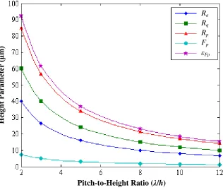
Figure 11. Roughness Parameters vs.

λ

/

h

for

λ

= 250 μm and

p

= 6 ...28

Figure 12. Ideal Surface Roughness Profiles for

h

= 50 μm,

λ

varies,

p

varies ...29

Figure 13. Roughness Parameters vs.

λ

/

h

for

λ

= 250 μm,

p

varies ...29

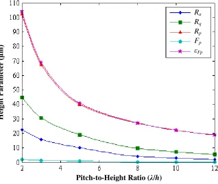
Figure 14. Roughness Parameters vs.

λ

/

h

for

h

= 50 μm,

p

varies ...30

Figure 15. Friction Factor vs. Aspect Ratio, Smooth Channel Correlation ...32

Figure 16. Friction Factor vs. Aspect Ratio, Constricted Flow Method,

Re

= 50 ...33

Figure 17. Friction Factor vs. Aspect Ratio, Wall Function Method,

Re

= 50 ...34

Figure 18. Comparison of Wall Function Method with Smooth Channel Correlation,

for Channel Separation

b

= 150 μm ...37

Figure 19. Comparison of Wall Function Method with Smooth Channel Correlation,

for Surface Profile

λ

/

h

= 5 ...38

Figure 20. Designed Roughness Profile,

h

= 50 μm,

λ

= 150 μm ...40

Figure 21. Laser Confocal Image of Wire EDM Result,

R

= 49.6 μm,

R

= 149.8 μm ....41

Figure 22. Curve-fit and Profile Data of Surface Designed for

h

= 50 μm,

λ

= 150 μm ...42

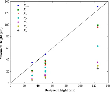
Figure 23. Measured Amplitude Parameters vs. Designed Height ...43

Figure 24. Shape Parameters vs. Power ...44

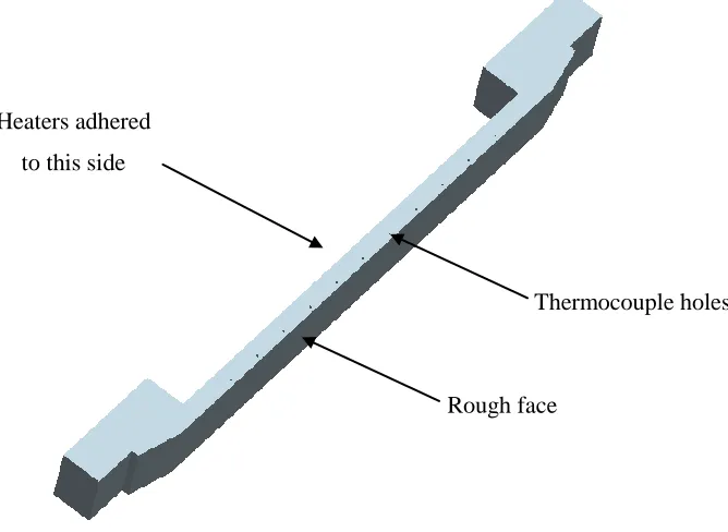
Figure 25. Solid Model of Roughness Test Piece ...45

vii

Figure 27. Solid Model of Microchannel Assembly ...47

Figure 28. Solid Model of Test Set Assembly (rear view) ...47

Figure 29. Schematic of Experimental Test Loop ...49

Figure 30. Smooth Channel Friction Factor vs. Reynolds Number, ...59

Figure 31. Smooth Channel Experimental vs. Theoretical Friction Factors ...60

Figure 32. Deviation in Channel Separation Measured Before and After Flow Testing ...61

Figure 33. Experimental Friction Factor vs. Reynolds Number,

λ

/

h

= 7 ...64

Figure 34. Experimental Friction Factor vs. Reynolds Number,

λ

/

h

= 8 ...65

Figure 35. Experimental Friction Factor vs. Reynolds Number,

λ

/

h

= 5 ...66

Figure 36. Experimental Friction Factor vs. Reynolds Number,

λ

/

h

= 3 ...67

Figure 37. Experimental Friction Factor vs. Reynolds Number,

λ

/

h

= 2 ...68

Figure 38. Experimental and Theoretical Friction Factor vs. Reynolds Number,

λ

/

h

= 7 ...70

Figure 39. Experimental and Theoretical Friction Factor vs. Reynolds Number,

λ

/

h

= 8 ...71

Figure 40. Experimental and Theoretical Friction Factor vs. Reynolds Number,

λ

/

h

= 5 ...72

Figure 41. Experimental and Theoretical Friction Factor vs. Reynolds Number,

λ

/

h

= 3 ...73

Figure 42. Experimental and Theoretical Friction Factor vs. Reynolds Number,

λ

/

h

= 2 ...74

Figure 43. Experimental Poiseuille Number vs. Channel Aspect Ratio ...76

viii

List of Tables

Table 1. Test Matrix Summary: Roughness Geometry - Designed ...39

Table 2. Test Matrix Summary: Channel Geometry - Designed ...39

Table 3. Roughness Parameters ...42

Table 4. Instrument Bias and Precision Error ...55

Table 5. Laminar and Turbulent Precision Error ...55

Table 6. Parameter Error ...56

Table 7. Measured Channel Geometry – Smooth Surfaces ...58

Table 8. Test Matrix Summary: Roughness Geometry - Measured ...61

Table 9. Test Matrix Summary: Channel Geometry - Measured...62

Table 10. Experimental Error ...75

ix

Nomenclature

Latin

A Area, surface or cross-sectional, as noted in the text

a Rectangular channel height, or

longer of the two dimensions

b Rectangular channel separation, or

smaller channel dimension

beff Effective channel separation

D Pipe diameter

Dh Hydraulic diameter

e Roughness size, used in the

Moody diagram [1]

Fp Average floor profile

(alternatively named FdRa)

f Friction factor

f(x) Lower wall function

g Gravity

g(x) Upper wall function

h Roughness height, wall function

method

k Roughness height, as defined by

Von Mises [2]

P Pressure

Q Volumetric flow rate

r Pipe radius

Ra Average roughness

Rc Average height

RΔq RMS tilt

Re Reynolds number

Rku Kurtosis

Rp Maximum peak height

Rq Root-mean-square (RMS)

roughness

Rsk Skew

RSM Mean spacing of peaks

Rv Minimum valley height

Rz Maximum or ten-point-peak

height

u x-component of velocity

v y-component of velocity

w z-component of velocity

Greek

α Channel aspect ratio; smaller dimension divided by larger

δ boundary layer thickness

Δa Mean slope of roughness profile

εFp Roughness height parameter, for

constricted flow model [3]

λ Roughness pitch

μ Dynamic viscosity

ρ Density

Subscripts

1

1

Introduction

The drive for understanding the fundamentals of microfluidics is not a new topic of discussion, as microchannels have been in use since the 1960‟s. However, the recent increase in

applications for microchannels has spurred the need for ongoing research.

Microchannel dimensions permit very high surface-area-to-volume ratios, greatly enhancing

heat and mass transfer, as well as chemical reactivity. The enhanced heat transfer makes

microchannel heat exchangers (MHE‟s) ideal in electronics cooling applications. In particular, the small footprints of MHE‟s make them ideal for cooling the densely packed processor and memory

units in servers and super computers. Some companies are currently developing microchannel

reactors, similar to MHE‟s, in which reaction conditions can be precisely controlled for processes

such as hydrogen production, conversion of natural gas into synthetic fuel, and the production of

household chemicals. Most of these devices are composed of arrays of parallel channels, with critical

dimensions, for microchannel reactors for example, ranging from 0.25 to 5 mm [4]. Bio-related

applications for microchannels include drug delivery research and detection and separation of

pathogens (viral, bacterial, and fungal) such as E. coli. Microchannel technology also allows for

accurate simulation of chemical diffusion in the blood, brain tissue, lung tissue, etc. Overall

advantages of using microchannels in industrial applications include increased product yields,

improved energy efficiency, smaller device footprints, and reduced capital costs. Fundamental

research on microscale transport processes is therefore required for further improvement and

implementation of microchannel technology.

A major difficulty in microfluidic devices, and the primary topic of this work, is that of

surface roughness. All surfaces possess natural or random roughness which results from

manufacturing processes. Inside any channel one may expect to find the walls are neither smooth nor

uniformly rough, but may have large burrs or gouges in various locations along the length of the

channel. This random roughness is typically smaller than the boundary layer thickness in internal

macroscale or large-scale flows. Therefore, it is assumed to have negligible influence in the laminar

flow regime, although it may take effect in turbulent flow if its height is larger than the viscous

boundary layer [5]. At the microscale level, where the channel walls are very closely spaced, the

height of individual asperities may be on the order of the channel dimensions. High roughness can

2

Surface roughness is typically characterized by the use of average amplitude parameters.

These conventional amplitude parameters are in common use because they are simple to calculate and

provide a sufficient description of natural roughness in macroscale applications. In order to

understand the effect of asperity height, slope, density, etc. of roughness on fluid flow, it is useful to

consider structured roughness so as to both control and measure those aspects of surface geometry

individually. The average amplitude parameters which are sufficient for uniform roughness are

3

2

Related Work

2.1

Historical Perspective

Since Darcy identified the dependence of internal fluid flow on pipe diameter, inclination,

and surface type in the 1800‟s [6], much effort has gone into experimental and theoretical

assessments of the effects of roughness on internal flows. In the early 1900‟s, Von Mises highlighted

the significance of relative roughness, which he defined as the ratio of roughness “size” to pipe

radius, k/r [2]. Hopf [7] and Fromm [8] later performed flow experiments on rectangular channels

with various types of roughness. They classified surface types based on roughness aspect ratios and

concluded that friction factor and Reynolds number are dependent on the surface type, differentiated

by the roughness pitch-to-height ratio, λ/h, for repeating roughness structures. In an attempt to expand

the understanding of flow in rough pipes at the time, Nikuradse performed exhaustive experiments

assessing a complete range of Reynolds numbers for various k/r values, while maintaining geometric

similitude in pipe geometries, resulting in an enormous database for frictional flow in pipes [9]. In

1939, Colebrook developed the general (and well-known) formula for friction factor at high Reynolds

numbers [10]. With Nikuradse‟s experimental results and Colebrook‟s turbulent flow formula, Moody

[1] constructed a convenient means, in graphical form, for estimating friction factors based on relative

roughness and Reynolds number, making the Darcy-Weisbach equation more readily applicable.

The Moody diagram allows for prediction of fluid behavior in macroscale pipes, and has been

in use in both academic and industry settings for decades. The diagram is limited to relative

roughness values of 5% and lower, or e/D < 0.05, however, and indicates that roughness of any size

has no effect on friction factors in the laminar flow regime. This conclusion that roughness takes no

effect in laminar flows is still pervasive today in that the flow in conventional-sized pipes and

channels is typically turbulent, so the variance in the friction factors for laminar flows are of less

practical importance. Interest in microscale phenomena has increased in the recent past due to its

usefulness for passive enhancement of microfluidic devices. With the increase in the use of

microscale geometries in various applications, and because flows in microscale pipes and ducts are

often laminar, the study of laminar flow in roughened microchannels is of significant importance.

Experiments performed since the 1980‟s indicate that as the pipe size decreases there is significant

4

2.2

Channel Geometry

Early research on internal flows focused on circular ducts or conventional pipes, as was the

case with the data used to generate the Moody diagram. For fully developed, laminar flow in circular

ducts, the Darcy friction factor may be defined as 64/ReD, where ReD is the Reynolds number

calculated using the pipe diameter as the characteristic length. This definition of laminar friction

factor does not hold true for non-circular geometries, since the wall shear varies around the perimeter

of the duct. In order to extend conventional correlations for non-circular geometries, the hydraulic

diameter may be used in place of the characteristic length;

P A

D_h 4

where A is the cross-sectional area and P is the wetted perimeter, or the length of the wall in contact

with the fluid flowing through the cross-section. For a rectangular cross-section in which one side is

significantly smaller than the other, Dh limits to twice the smaller dimension. This concept of

hydraulic diameter is used simply to extend existing empirical correlations for pipe flow to

non-circular geometries, and to represent the characteristic length scale in fluid mechanics.

Throughout the 1970‟s, Shah worked to analyze the variation of fully developed, laminar

flow friction factors in smooth ducts of various cross sectional geometries using a

least-squares-matching technique [12, 13]. His work resulted in a compilation of analytical solutions for flow

friction based on data from over 300 sources for 25 duct geometries. These solutions are still used for

comparison to this day, and are likewise used for smooth channel comparison in this work.

In more recent literature, researchers have reported that friction factors in non-circular

geometries begin to differ from Shah‟s findings as the channel size decreases to the microscale level.

In gas flows, the discrepancy may be attributed to slip flow at the boundaries, but this does not

explain the difference for incompressible flows. Prior works on liquid flow in microchannels have

reported significant increases [14-17] or decreases [18, 19] in friction factors from conventional

laminar theory, while others reported negligible deviations [20-24]. In addition to these, other authors

have reported increases in friction factors for some geometries or aspect ratios, but decreases for

others [25, 26]. Many of these authors highlighted the role of wall roughness in their observed

5

While a wide variety of channel shapes and sizes have been investigated in literature, the

classification of channel size (i.e. microscale, miniscale, etc.) is still not definitive. In many cases, the

term microchannel may be applied to channels having a hydraulic diameter greater than 1 mm. The

classification scheme recommended by Kandlikar and Grande [27] indicates delineations based on

molecular mean free path considerations for single phase gas flow, and surface tension effects in two

phase flow. Their conclusion result in the following classifications:

Conventional channels: Dh > 3 mm

Minichannels: 200 μm < Dh ≤ 3 mm

Microchannels: 10 μm < Dh ≤ 200 μm

An earlier classification scheme was defined arbitrarily for size-range classification in

industry by Mehendale et al. [28] as follows:

Conventional channels: Dh > 6 mm

Compact Passages: 1 mm < Dh ≤ 6 mm

Mesochannels: 100 μm < Dh ≤ 1 mm

Microchannels: 1 μm < Dh ≤ 100 μm

Scale may indicate both the channel size and roughness size. Through the use of either of

these schemes, it is revealed that the majority of conventional microfluidic devices are in actuality

comprised of minichannels. Size classification becomes more complicated with channels of

non-circular cross-sections, as channel shape and aspect ratio are known to have significant effects on

flow behavior in channels of all sizes [12, 13]. It is recommended by Kandlikar et al. [11] that the

minimum dimension of any given channel be used in place of the hydraulic diameter. That is, for

rectangular channels the shorter side of the rectangle will replace the hydraulic diameter in

calculations and table look-ups. Bahrami et al. [29] recommend using the square root of a channel‟s

cross-sectional area as the characteristic length, as they claim it is superior to the hydraulic diameter.

Although the effects of channel geometry on internal fluid flow have been studied extensively

in literature, the channel size effects are still not definitive. It is generally agreed upon, however, that

surface roughness must be understood in small-scale flows. The majority of pre-1990‟s literature is

concerned with the general aspects of flows over rough walls, while more recent research has

emphasized the differences between various types of roughness. These types are separated here into

6

2.3

Uniform Roughness

The surface roughness used in many experiments can be classified as uniform or Gaussian

roughness. That is, the amplitude density distribution for the data obtained from a profilometer,

microscope, or other metrology device is a normal or Gaussian distribution. When glass is etched or

metals are abraded, the outcome is frequently Gaussian. The roughness that results naturally from

various machining and manufacture techniques is random, but frequently Gaussian. The difference is

that random roughness is not controlled or deliberate, whereas etching or polishing is done in order to

obtain a desired surface finish. A skewed distribution is indicative of prominent peaks or valleys

across a surface, but in general the same geometry would be found uniformly across an etched or grit

blasted surface.

The Moody diagram is based heavily on experimental data for uniformly rough surfaces.

Nikuradse, for example, sifted and re-sifted sand so that the grain diameters were approximately the

same, then used a lacquer to adhere the sand to the inner surfaces of pipes [9]. Since then, authors

have attempted to equate surface roughness to an equivalent sand grain roughness. Such an approach

to roughness characterization is questionable as the method of gluing sand to a surface may not result in roughness that is the same size as the sand grains, nor could repeating Nikuradse‟s method result in

the same density or distribution of grains on the surface. Any slight difference in coating or drying the

sand could result in different flow resistance. While the size of uniform roughness may be controlled

in this technique, the distribution is entirely uniform across the surface and is difficult to characterize

by anything other than amplitude parameters, hence the desire to use an equivalent sand grain

roughness for comparison.

Existing roughness parameters primarily serve to describe natural or uniform roughness by

the average or extreme height. Standard amplitude parameters include the average roughness, Ra,

which is the arithmetic mean of surface height values, and the root-mean-square (RMS) roughness,

Rq, which is the standard deviation of the height distribution. Line measurements are represented by

R, whereas surface measurements are represented by S. Most amplitude parameters use the average

roughness as a reference line. Extreme height parameters, for example, represent the highest peaks or

deepest gouges in a surface relative to the mean line. In Nikuradse‟s experiments, the use of the sand

grain diameter for the roughness value is comparable to using an extreme amplitude parameter to

represent the surface in that the sand particles would not actually project into the boundary layer to

their full diameter due to the laquer coating. Amplitude parameters are useful for surface specification

7

Alternative roughness parameters may contribute to the prediction of hydraulic performance,

but are not in common use for fluid flow applications. The skew of a surface, Rsk, represents the

symmetry of that profile about its meanline, indicating whether it possesses many sharp peaks

(positive skewness), sharp valleys (negative skewness), or is a Gaussian distribution (Rsk = 0).

Kurtosis, Rku, represents the peakedness of a surface, qualifying the flatness of the amplitude density

distribution. A leptokurtic surface (Rku > 3) possesses frequent extreme peaks and valleys, as opposed

to a platykurtic surface which exhibits infrequent or small deviations. There are also parameters for

counting the number of times a profile crosses a threshold, and for evaluating the density or slopes of

peaks. These and many other spatial or functional parameters have potential for use in predicting

surface effects on fluid flows.

Menezes et al. [30] roughened steel surfaces with wet and dry emery paper in various

patterns in order to correlate twenty five existing roughness parameters, including skew and kurtosis,

with the coefficient of friction for each surface under lubricated conditions. He found that the

performance of each plate was independent of the average roughness Ra, but correlated well with the

mean slope of the profile Δa for every surface. This parameter is the arithmetic mean of the slopes

between every pair of successive points of a roughness profile, giving an indication of the shape of

the profile. Although it compared well in the reported experiments, it does not completely describe a

surface and may need to be combined with an amplitude or hybrid parameter. No conclusion was

made for the skew or kurtosis parameters, though it was implied that these were unable to be

correlated with the frictional coefficient.

In 2005, Kandlikar et al. [3] proposed the use of a constricted parameter for use in estimating

pressure drop in roughened microchannels. The parameter εFp is a function of the average roughness

and two other amplitude parameters, and serves to account more accurately for the extent to which

roughness elements project into the boundary layer. This constricted flow approach led to a modified

Moody diagram which covers higher relative roughness values and smaller hydraulic diameters. This

approach is valid provided that the roughness elements are closely spaced. There is still a need,

8

2.4

Structured Roughness

Structured or artificial roughness was studied at least as far back as the 1920‟s with Hopf and Fromm‟s saw-tooth style two-dimensional roughness [7, 8], followed by Schlichting‟s

three-dimensional arrays of spheres, cones, and angled roughness [31]. Structured roughness is obtained by

adding or removing material from a surface in a deliberate and precise way such that a two- or

three-dimensional pattern arises. Though the focus for these authors was on turbulent flow, they were some

of the pioneers in artificial roughness studies.

As there is no “universal” parameter for structured roughness, many researchers have resorted

to using roughness height values and relative roughness in order to assess and compare the effects of

different roughness geometries on fluid flow, even in recent literature. Schlichting, who used an

equivalent sand grain roughness in his study, also attempted to correlate the flow resistance with

roughness density, quantified by the projected roughness area normal to flow divided by the total

plate area. In 1952, Sams [32] experimented with structured roughness in laminar and turbulent flow

by threading and cross-threading macroscale pipes (D ≈ 12.7 mm). He concluded that the conventional “relative roughness” concept is not sufficiently representative of the effects of structured

roughness, specifically his square thread type roughness, on hydraulic performance. Though the

author went to great lengths to correlate friction factors with the square roughness height, width, and

spacing, the final outcomes were a series of empirical formulations.

Numerical simulations have been employed for assessing structured roughness effects in

microchannel flow by a number of researchers, either through the use of commercial CFD software or

by programming finite difference methods manually in languages such as FORTRAN or computing

environments like MATLAB, etc. Rawool et al. [33] simulated laminar air flow in microchannels

possessing two-dimensional transverse rib roughness, and systematically varied the roughness

cross-section from triangular to trapezoidal to rectangular, as well as varying the height and pitch, or

peak-to-peak distance. The authors found that the roughness pitch plays a definite role in fluid flow, in that

the friction factor increases as roughness elements are brought closer together, i.e. higher friction

factors for smaller pitch values. This was in addition to the roughness height effect already seen in

previous literature; friction factor increases as roughness height increases. Friction factors were also

found to be greater for triangular and rectangular geometries, and lower for trapezoidal roughness.

These results are in agreement with the numerical simulations of Wang et al. [34] and Sun and Faghri

9

Transition to turbulence is frequently correlated to the ratio of roughness height to boundary

layer thickness k/δ, which highlights the importance of the interaction of roughness elements with the

boundary layer. In a review on turbulent flows over transverse rib type roughness, Jiménez [36]

described two types of roughness; d-type and k-type, and a transitional roughness that occurs between

these two types. They d-type roughness was described as ribs closely spaced such that they can

sustain stable vortices (recirculation downstream of the roughness elements) that serve to isolate the

bulk flow from the roughness. The k-type roughness is sparser such that the flow separates at the top

of the roughness element and reattaches downstream, before reaching the next roughness element.

The vortices interact with the bulk flow for this sparse roughness, causing increased friction factors

and early transition to turbulence. Coleman et al. [37] experimentally and numerically assessed the

effect of transverse rib roughness pitch-to-height ratios, λ/h, on turbulent flow and identified “transitional” roughness, at λ/h ≈ 8, as having the most predominant effect on fluid flow. The authors

reported that values of λ/h < 5 indicate closely spaced ribs, d-type roughness, or skimming flow,

while λ/h > 5 indicate isolated roughness elements, k-type roughness, or interactive flow. In the

extremes where λ/h is significantly greater or less than 5, the roughness effect is expected to diminish.

Although these publications discussing roughness ratios focus on turbulent flows, the concept may

still hold true for microscale laminar flows.

2.5

Roughness Models

As stated previously, there are no theoretical differences between microscale and macroscale

flows for incompressible liquids. Some authors, however, have made modifications to conventional

theory in order to account for microscale roughness effects. In this section, a few of those models for

flow in rough microchannels are reviewed. These models were either developed for or have been

applied to steady, laminar, fully-developed liquid flows in microchannels possessing uniform or

structured roughness.

Mala and Li [38] proposed the roughness-viscosity model (RVM), in which the surface

roughness increases the fluid viscosity near the wall, accounting for the increase in friction factor in

laminar flow. The authors define roughness-viscosity as a function of distance from the wall, such

that the roughness-viscosity is zero at the center of the channel and a positive, non-zero, finite value

at the wall. The concept is that the surface roughness increases momentum transfer in the boundary

10

Sabry [39] took a unique approach that is reminiscent of the Cassie-Baxter model for surface

wetting; the liquid does not fully contact the rough walls, and gases are trapped between some

roughness elements. Conceptually, in this model, when flow separation occurs over roughness

elements, the flow will become separated from the wall by a thin film of gas. The author initially

assumed a “blanket” of gas of a specified thickness completely separates the bulk liquid from the

rough wall. Since, in actuality, a gas blanket could not completely separate the liquid from the solid, a

shielding coefficient was introduced into the model. This correction factor would range from 0 for no

entrained gas to 1 for total separation of liquid from solid. Though the concept may be of interest in

heat transfer applications, as a vapor blanket would be likely to occur and would insulate the flow,

this model does not address the variation in friction factor with roughness height, as has been

observed in previous literature.

Koo and Kleinstreuer [40], and Kleinstreuer and Koo [41], proposed a porous medium layer

(PML) model in which uniform or random surface roughness is represented by a porous region or

layer on the walls of a channel. The surface roughness (or PML) can increase or decrease the friction

factor, depending on the PML permeability. The authors found good agreement with previous data.

However, the model requires a number of unique and obscure parameters, such as porosity,

permeability, and resistance speed factor, resistance speed power, and resistance constant. Constraints

for the resistance variables were stated, but their exact definitions were not clear.

Expanding on the PML model, Gamrat et al [42, 43] developed a roughness layer model

(RLM) in which they employed a discrete element approach to represent roughness at the wall. The

authors used two effective roughness height parameters that are dependent on two dimensionless parameters; porosity of the “rough layer” and roughness height normalized by roughness spacing. The

authors reported good agreement with experimental data for both uniform and structured roughness.

But, the model is semi-empirical, as a drag coefficient must be obtained experimentally.

2.6

Objectives

Definite departure from conventional laminar theory has been identified in numerous

experiment-based publications. Vast portions of the experimental works have resulted in empirical

relations, scaling factors, etc., and these correlations are not universally applicable across the full

11

works result in scaling models or require correction factors. Although it is intuitive that flow over a

rough surface will experience greater drag than a smooth surface, it is still unclear when, where, and

how a rough surface will begin to affect the bulk flow.

The study described herein deals with laminar water flow in rectangular channels of small

aspect ratios, primarily in what may be considered the minichannel range, but touches on the

microscale regime. Structured roughness is evaluated for its controllability of pitch and height. This

work is an extension of a series of experiments performed by Brackbill [44] with saw-tooth roughness

in rectangular microchannels. Standard amplitude parameters were evaluated as well as spatial and

functional parameters in order to determine a combination of parameters relevant to structured

roughness surface description. The relative roughness, εFp/Dh, and the ratio of roughness height to

channel separation, h/b, were also assessed for comparison with prior works. It is shown here that

flow between rough walls can be modeled without the detailed computation of the flow around the

12

3

Theoretical Model

Two-dimensional structured roughness was studied for its controllability of height, pitch, and

slope of periodic peaks. A theoretical flow model that incorporates descriptive roughness parameters

was developed, with focus on fully developed laminar flow.

3.1

Fundamental Equations and Computational Domain

The Navier-Stokes (N-S) equations for an incompressible Newtonian fluid form the

foundation for the theoretical treatment of the microscale problem presented here. The result of the

analysis provides pressure as a function of velocity, fluid properties, and channel and roughness

geometry. In addition, the continuity equation was used to complete the relationship between

volumetric flow rate and pressure terms. The internal two-dimensional flow was assumed to be steady

and fully developed, so that inlet and outlet effects may be neglected. For further simplification, fluid

properties were assumed to be constant.

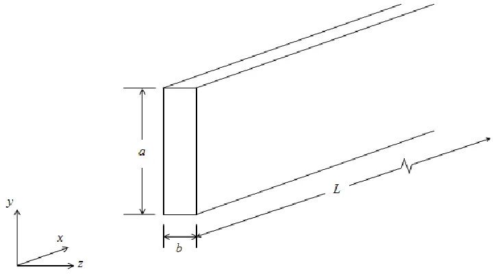
Channel orientation and geometry are displayed in Figure 1 below. Fluid flow is in the

positive x-direction, transverse rib roughness is in the x-y plane, and gravity acts in the negative y

-direction. The channel separation b is significantly less than the channel length L, and the channel

aspect ratio is small, such that the flow is comparable to flow between infinite parallel plates.

13

The computational domain is the region between the rough walls, in the x-z plane. The

boundaries for the flow is the transverse rib roughness, represented by the functions f(x) and g(x) for

the lower and upper walls, respectively, as seen in Figure 2. This periodic roughness is described by

its pitch λ and height h. Channel separation b is the difference between wall functions f(x) and g(x).

The treatment of the separation b is discussed in the Surface Roughness and Channel Separation

section. The limits of integration in the x-direction are from 0 to L.

Figure 2. Computational Domain

3.2

Assumptions and System of Equations

This is a two-dimensional analysis, for which the velocity vector is

u





u

i

ˆ



w

k

ˆ

which is validated in this section. The fluid is an incompressible liquid, for which the density and

viscosity are constant. Gravity acts in the y-direction only, perpendicular to the computational domain

shown in Figure 2 above. Inlet and outlet effects are neglected. The no-slip boundary condition is

applied, i.e. velocity at the walls, where z  f(x) and z g(x), is zero. In addition, it is assumed

that the pressure at the inlet and outlet, or P0 and PL, respectively, are known.

The momentum equation, Newton‟s second law of motion, balances the acceleration of a

14

expresses conservation of mass for a constant density fluid. These comprise the system of equations

used for the current analysis:

0 :       z w x u Continuity

















































































































































z

w

w

x

w

u

z

w

x

w

z

P

component

z

y

P

g

component

y

z

u

w

x

u

u

z

u

x

u

x

P

component

x

S

N











:

0

:

:

3.2.1 Lubrication Approximation

To solve the full N-S equations requires the use of computational fluid dynamics. In this

analysis, the lubrication approximation was applied for simplification by assuming that the slope of

the trajectory of fluid elements is small. That is, velocity w in the z-direction is significantly less than

velocity u in the x-direction. Figure 3 provides a visual representation of this assumption.

Figure 3. Trajectory of a Fluid Particle and its Velocity Components

Also referred to as the small slope approximation, it may be interpreted as; the slope of the

boundaries is small at every point, such that ( ) 1 

 x

x f

and ( ) 1 

 x

x g

. This approximation is

often applied to flow fields in which the fluid is forced to move between two closely spaced surfaces,

15

3.2.2 Simplified System of Equations

Application of the lubrication approximation makes no change to the continuity equation, but

reduces the conservation of momentum equations thus:

                        0 : : : ₂ 2 z P component z g y P component y z u x P component x S N





In the x-direction, all that remains is the viscous effects. Gravity only takes effect in the y

-direction and may be used to assess variation of velocity in the y-direction. All inertial terms drop out

due to the lubrication approximation. The lack of inertia implies very low Reynolds numbers (Stoke‟s

flow) or flow in a slot of low relative roughness (small slope).

Integrating the x- and y-components of the simplified N-S equations and applying the no-slip

boundary conditions yields the following:

) (x p gy

P









u  

  



Equation 1 allows for an understanding of the effect of gravity on flow. It may be used to

evaluate changes in the flow field in the y-direction. Equation 2 represents the bulk flow velocity

profile in the absence of inertia. In laminar flow, if the channel separation b is significantly less than

the length L, then the flow is approximately parabolic, as is this bulk profile. In an extended analysis,

in section 3.5, this velocity profile serves as a trial function in an augmented lubrication

approximation in which the inertial terms in the x-component are not discounted.

Integration of the continuity equation across the channel separation brings about a volumetric

flow rate per unit depth relation. Applying Leibniz Rule, and utilizing equation 2 as an initial

approximation for the velocity profile results in the following pressure–flow relation:





P _{ }

16

Rearranging for the differential pressure term as a function of flow:





)

(

)

(

1

12

x

f

x

g

a

Q

x

P













Integrating this differential equation along a specified length results in an equation for

pressure-drop as a function of flow rate, viscosity, and the boundaries or wall function equations:

















x

x

f

x

g

a

Q

P

P

)

(

)

(

1

12



From here, equations for g(x) and f(x) are used to evaluate the integral and thereby predict the

pressure drop along the length of rough channel. These two equations are the wall functions that

represent structured two-dimensional roughness, and so this approach is referred to as the wall

function method.

3.3

Wall Function Method

Pressure drop along a length of rectangular channel may now be predicted, provided that the

channel and roughness geometries, fluid properties, and flow rate are known. Because the intention of

this study was to investigate the effects of structured roughness on laminar fluid flow, it was

necessary to utilize these wall functions f(x) and g(x) in such a way that the height and pitch of evenly

spaced peaks may be systematically varied.

3.3.1 Structured Roughness

The form of the roughness chosen for this study was obtained through curve-fitting of

existing two-dimensionally rough surfaces, possessing “saw-tooth” style roughness. These surfaces

and the curve-fitting exercise are discussed further in Section 4.1, Saw-tooth Roughness. The

equation format for the periodic roughness is:

 

2

cos x b

h x

f p 

17

where h is the height of roughness elements, λ is the pitch or peak-to-peak spacing, p is the power on

the cosine which controls the slope of the peaks, and b is the root channel separation, measured

valley-to-valley. The opposing wall g(x) is the negative of equation 6 (refer to Figure 2). Thus, the

difference between these two functions results in the root channel separation minus a power sinusoid

that is a function of x.

 

 f x b h x x g p





This form of two-dimensional roughness is convenient in that it allows for control of all

parameters of interest, such that any one variable may be manipulated while keeping the remaining

geometries constant. To evaluate the effect of alignment of roughness peaks on fluid flow, a phase

shift variable may be added into the cosine function of one of the walls.

Implementing this style of roughness is not trivial for the theoretical model at hand. The

integral in equation 5 is difficult to solve exactly, and requires the use of averaging techniques when

boundaries of the form of equation 6 are used for the wall function input. Therefore, the Gaussian

quadrature rule was used to approximate the integral. Code was written in MATLAB in order to

expedite the analysis of an extensive combination of surface profiles, channel geometries, and flow

rates. A sample of this code can be found in Appendix A.

3.4

Constricted Flow Method

In prior works by Brackbill [44] and Brackbill and Kandlikar [45, 46] an effective channel

separation was used for evaluation of flow behavior. To achieve this, the integral portion of equation

5 was simplified by taking f(x) and g(x) to be constant values, i.e. the channel walls are essentially

hydraulically smooth, thus:





0 3

)

(

)

(

1

b

L

x

x

f

x

g









The effective separation, beff, is then defined as:

) ( ) (x f x g

18 Equation 5 becomes:

3

0

12

eff L

b

L

a

Q

P

P









This formulation has been found to be valid for macroscale channels, or channels possessing

low relative roughness. For microscale flows, however, surface roughness must be accounted for.

Average amplitude parameters currently in use have been shown to be ineffective by Perry et al. [48],

therefore the channel separation must be given careful consideration.

3.4.1 Surface Roughness and Channel Separation

Amplitude parameters such as the average roughness, Ra, and root-mean-square roughness,

Rq, are typically used to describe surfaces of random or uniform roughness, like the sand grain

roughness used by Nikuradse. Simple average parameters and the concept of “relative roughness,”

however, are insufficient for structured two-dimensional roughness [32].

A sample of structured roughness, machined via ball end mill on CNC, and its associated Ra

and Rq values are shown in Figure 4. This shows how utilizing these parameters would fail to account

for the significant peaks in the profile, which may project into the boundary layer.

Figure 4. Profilometer Data for 815 μm Pitch Saw-tooth Roughness Profile with Amplitude Parameters and Constricted Parameter, εFp

Profile Ra Rq Fp Rp εFp

x (μm)

z

(

μ

m

19

Kandlikar et al. [3] set forth a method for assessing a surface of significant random roughness

or structured roughness. This new roughness factor, referred to as the constricted flow parameter, is a

function of the average parameters typically obtained through surface analysis:





p p Fp

F

R

F

R









-M ax



(11)

where Max is the single highest point obtained from one evaluation length of any given profile. The

floor profile, Fp, also called FdRa, is defined as the average of all points below the mean line, Ra,

which is simply the arithmetic mean of the height of all points along a profile. These additional values

for the 815 μm surface are also shown in Figure 4.

Figure 5. Representative Channel and Roughness Geometry; h = 100 μm, λ = 400 μm, b = 400 μm

The constricted parameter was used to develop a constricted channel separation bcf for use in

place of beff in equation 10. This constricted separation is calculated as:

Fp

cf b

b  2



where b is the root separation between two rough walls, measured between the floor profiles (Fp) of

opposing surfaces. By this definition, any amplitude parameter could be used to “constrict” the

channel separation. Figure 5 shows a sample cross-section of a channel possessing the ideal Profile

Ra εFp

x (μm)

z

(

μ

m

20

sinusoidal structured roughness discussed previously, with its constricted separation and average

roughness separation. In this figure, it can be seen that using the average roughness to define the

channel separation does not entirely account for the peaks.

In previous studies [45, 46], the constricted parameter was successfully used to fit

experimental data to conventional laminar theory by using the constricted separation bcf in place of

beff, in equation 10. This constricted flow method is effective in accounting for natural or random

roughness, as well as some forms of structured roughness. It is not a strong function of roughness

pitch, however, which is an aspect of structured roughness that is known to have a significant effect

on fluid flow. Nor does the constricted parameter account for shape or alignment of roughness peaks.

Therefore, to improve the understanding of the effects of structured two-dimensional roughness, it

becomes necessary to consider all aspects of roughness geometry by representing the wall roughness

as an exact function of x.

3.5

Further Theoretical Analysis

For relatively high Reynolds numbers, flow can be divided into a bulk region of inviscid flow

unaffected by viscosity, and a region close to the wall where viscosity is significant (the boundary

layer). The inertial term in the x-component of the N-S equation may be non-negligible. This further

analysis allows us to understand the impact of the lubrication approximation itself without the added

complication of unknown velocity profile assumptions. Also, it allows for examination of the velocity

profile from the boundary layer solution and the behavior of the inertial term as the velocity increases

and hydraulic diameter decreases.

An augmented velocity profile is required for this analysis. Incorporating the differential

pressure function from the prior analysis (equation 4) into the initial velocity profile approximation

(equation 2) yields:



(

)

(

)





(

)



(

)



6

3

z

g

x

z

f

x

x

f

x

g

a

Q

u









In this equation, velocity is strictly a function of flow rate and wall geometry, and varies with

x and z. The profile is parabolic and the equation satisfies the boundary conditions and continuity

21

Using an augmented lubrication approximation in which the inertial term is not neglected, the

x-component of N-S equation is:





































z

u

w

x

u

u

z

u

x

P





2 2

(14)

Through the use of u-substitution and Leibniz Rule, this differential equation simplifies to:







P





(15)

If the velocity profile is known, this equation may be solved for a pressure–flow relation that

includes the inertial term. Therefore, we use the velocity profile developed previously (equation 13)

as a trial function, yielding the following pressure-drop equation:































































L

x

x

f

x

g

x

x

f

x

x

g

a

Q

x

x

f

x

g

a

Q

P

P

)

(

)

(

)

(

)

(

5

6

)

(

)

(

1

12





(16)

The first term of this equation is the same as the previous analysis (equation 5). The inertial

integral is not trivial to solve, however, once the trigonometric profile (equation 6) is applied.

Examining the limits of this analysis can indicate the potential usefulness of this augmented analysis.

If inertia were negligible, as with low Reynolds number flows, this formulation would limit back to

the lubrication approximation equation (equation 5). Similarly, in the smooth wall case, f(x) and g(x)

are constants, the derivatives of which are zero. The inertial integral will then yield a negligible

constant. Thus, the formulation is consistent with the boundary layer analysis for the case of

hydraulically smooth walls. Overall, these limits indicate that the analysis has potential as an

22

3.6

Application of Theory

In order to test the theoretical pressure loss equation (equation 5) and to compare it with

existing laminar flow models, friction factors must be evaluated for varying Reynolds numbers. To

this end, the pressure-loss form of the Darcy-Weisbach equation, or Darcy friction factor, was used to

calculate experimental friction factors:

2

2

















A

Q

D

L

P

f



where Dh is the hydraulic diameter, calculated as four times the cross-sectional area divided by the

wetted perimeter: b a ab D_h 

 2 (18)

The Darcy-Weisbach equation was also used to calculate theoretical friction factors with ΔP

obtained from the wall function method. For comparison with conventional laminar theory, the

correlation for friction factors in smooth, rectangular ducts, from Kakaç et al. [51], was also

evaluated: ) 2537 . 0 9564 . 0 7012 . 1 9467 . 1 3553 . 1 1 ( Re

24 













f (19)

where the aspect ratio is calculated as the channel width divided by channel height:

a b 



Reynolds number was calculated as:

A

QD







Re

The hydraulic diameter and cross-sectional area may be “constricted” by using the constricted

separation in place of the root separation. Similarly, Reynolds number may be constricted by using

the constricted hydraulic diameter and area. Constricted friction factors may be calculated by using

23

4

Preliminary Results

This chapter presents the results of comparison of available data with the theoretical model,

prior to the design and manufacture of a new test set and roughness pieces. In addition, the roughness

profile, equation 6, was evaluated in order to optimize the profile and understand the effects of each

variable on roughness amplitude parameters.

4.1

Saw-tooth Roughness

Experimental data from previous tests by Brackbill [44] were used for comparison with the

wall function method detailed above. Initial validation of the experimental setup was reported for the

hydraulically smooth channel case. Channel separation values were 200, 300, and 500 μm. Flow rates

in these experiments were varied to cover the range of Reynolds numbers from 487 to 2322. Friction

factors were calculated by Brackbill using equation 19 for laminar theory and the constricted Darcy

friction factor for experimental values. Figure 6 shows the comparison between Brackbill‟s

experimental data for hydraulically smooth channels and the smooth channel correlation (Equation

19). For each of these three channel separations, error was less than 4% at all flow rates.

Figure 6. Smooth Channel Validation of Previous Experimental Setup

Laminar Theory bcf = 200 μm bcf = 300 μm bcf = 500 μm

Re

24

The style of two-dimensional roughness examined by Brackbill is referred to as “saw-tooth”

roughness. The surfaces possessed evenly spaced peaks, and were described by the roughness height

and pitch. A sample of profilometer data from one such saw-tooth surface is shown in Figure 7 below.

This surface would form one wall of a channel, as shown in Figure 5.

Figure 7. Saw-tooth Roughness Profile with Height Parameters, λ = 503 μm

This figure includes the standard average amplitude parameters, Ra and Rq, as well as the

constricted parameter εFp and its components, Rp and Fp, obtained from the profilometer data. It is

shown that of all these parameters, none fully account for the peak heights, though the constricted

parameter is closest. The peaks for this surface were designed to be 50 µm tall, but the constricted

parameter was found to be 38.75 µm. Amplitude parameters do not account for the distance between

the major peaks, so it becomes necessary to use spatial parameters. However, due to the smaller peaks

between those major peaks, on the order of 20 µm tall, the standard spatial parameters were incapable

of characterizing the major peaks. The roughness between the major peaks has the added effect of

skewing height parameters and complicating the measurement of the root channel separation.

In order to apply the wall function method, the “saw-tooth” surfaces were fit with smooth,

continuous polynomials. This was achieved by examining the profiles and formulating sinusoidal Profile Ra Rq Fp Rp εFp

x (μm)

z

(

μ

m

25

functions that fit the curvature. Through a series of curve-fitting exercises, initially using complex

combinations of trigonometric functions, it was quickly determined that the minor peaks could not be

accounted for by any continuous stable function, and so equation 6 was developed. Leaving all

coefficients as variables, the least sum of squares method was used in conjunction with Excel‟s

Solver tool to obtain a best fit. A sample image of the same profilometer data shown in Figure 7 and

its corresponding curve-fit are shown below in Figure 8.

Figure 8. Curve Fit of 503 μm Pitch Saw-tooth Roughness Profile

Figure 8 is one example of a smooth curve of the form of equation 6 (shown in orange) fit to

profilometer data from saw-tooth roughness (shown in black). The height obtained for the curve fit of

this profile is 37.2 µm and the pitch is 416.7 µm. The “floor” of the profile was taken to be the same

as the Fp parameter, shown in Figure 7, but was allowed to vary slightly in order to obtain a best fit.

Although the difference between the curve fit and the surface data was minimized, it is clear that it

does not provide a perfect fit as it neglects the roughness in the valleys between the major peaks. This

minor roughness may be non-negligible in microscale flows, particularly considering interactive flow.

Though the curve does not provide an exact fit, the friction factors obtained through the wall

function method provided an excellent prediction of the channel‟s hydraulic performance for two

channel separations. The two figures below show the un-constricted laminar experimental data

x (μm)

z

(

μ

m

)

26

obtained by Brackbill [44] for two channel separations of the 503 µm pitch surface; b = 300 and 400

µm. The plots include the conventional laminar theory line (equation 19), and the line predicted by

the wall function method based on the curve fit of Figure 8.

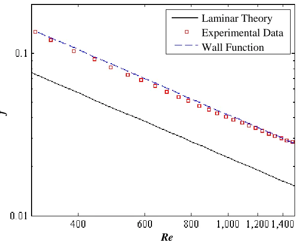
Figure 9. f vs. Re for 503 μm Pitch Surface, b = 400 μm

Figure 10. f vs. Re for 503 μm Pitch Surface, b = 300 μm Re

f

Re

f

Laminar Theory Experimental Data Wall Function

Re

f

27

The experimental data for b = 300 µm are an average of 76% greater than the friction factors

predicted by laminar theory, and for b = 400 µm about 65% greater. The data fits the lines predicted

by the wall function method to within 4% for b = 300 µm and within 10% for b = 400 µm. However,

the wall function method under-predicts the 400µm channel size case and over-predicts the 300 µm.