The Effect of cylindrical obstructions on the fluid flow in narrow rectangular channels

Rochester Institute of Technology

RIT Scholar Works

Theses

Thesis/Dissertation Collections

8-1-1996

The Effect of cylindrical obstructions on the fluid

flow in narrow rectangular channels

Gary Compagna

Follow this and additional works at:

http://scholarworks.rit.edu/theses

Recommended Citation

The Effect of Cylindrical Obstructions on the Fluid Flow

in Narrow Rectangular Channels

by

Gary L. Compagna

A Thesis submitted in partial fulfillment

of the requirements for the degree of

Master of Science in Mechanical Engineering

Approved By:

Professor S. Kandlikar

Professor

A.

Nye

Professor

A.

Ogut

Professor C. Haines

DEPARTMENT OF MECHANICAL ENGINEERING

COLLEGE OF ENGINEERING

ROCHESTER INSTITUTE OF TECHNOLOGY

PERMISSION GRANTED

I, Gary

L.

Compagna, hereby grant pennission to the Wallace Memorial Library of the

Rochester Institute of Technology to reproduce my thesis entitled "The Effect of Cylindrical

Obstructions on the Fluid Flow in Narrow Rectangular Channels" in whole or in part. Any

reproduction will not be for commercial use or profit.

August 31, 1996

ACKNOWLEDGMENTS

This

work could not

have

been

completed without

the

assistance and

understanding

of

several

outstanding individuals.

Kiran Kumar

and

Dr.

Sung-Eun

Kim

from

Creare,

Inc.

providedassistance

that

included

helping

with

FLUENT

software

issues

and also with

understanding

of

the

fluid

mechanics

involved

in

this

problem.

A

special

thanks

goes

to

Satish Kandlikar

without whose gentle

pushing

and

understanding

Table

of

Contents

Page

LIST

OF

FIGURES

iii

LIST OF

TABLES

vi

LIST OF

SYMBOLS

vii

ABSTRACT

1

1.

INTRODUCTION

2

1.1

APPLICABILITY

OF HELE-SHAW FLOW

5

1.2

APPLICATIONS

9

1.2.1 POLYMERASE CHAIN REACTION DETECTION POUCH

9

1.2.2 OTHER

APPLICATIONS

10

1.3

PROBLEM DEFINITION

12

1.4

OBJECTIVES

OF THE PRESENT WORK

15

2. LITERATURE REVIEW

16

2.1

BASIC

GOVERNING EQUATIONS

26

2.1.1 FLUID FLOW

GOVERMNG EQUATIONS

26

2.1.2 POTENTIAL FLOW

28

3. THEORETICAL ANALYSIS

37

3.1

FLUID FLOW IN RECTANGULAR DUCTS

37

3.2

INVISCID IRROTATIONAL FLOW IN TWO

DIMENSIONAL

FLOW

41

3.2. 1 POTENTIAL FLOW FIELD FOR UNIFORM FLOW OVER A

CYLINDER....

42

3.2.2

POTENTIAL

FLOW RESULTS

USING METHOD OF IMAGES

44

4.

NUMERICAL

ANALYSIS METHOD

50

Page

4.1.2

2-D FLUID FLOW WITH CYLINDRICAL OBSTRUCTION

57

4.2

VERIFICATION

OF

NUMERICAL

ANALYSIS

81

4.2.1

2-D FLOW AROUND

CYLINDER

COMPARISON WITH FLUENT

81

4.2.2 FLUENT COMPARISONS

FOR VISCOUS FLOW OVER A CYLINDER

91

4.2.3 VISCOUS

FLOW

COMPARISON

FOR DIFFERENT GRID

FORMULATIONS

97

4.2.4 3-D

VISCOUS

FLOW COMPARISON TO FLUENT RESULTS IN

NARROW RECTANGULAR DUCTS

99

5. RESULTS FOR 3-D FLOW

104

5.1

BASELINE 3-D RESULT

104

5.2

FLOW UNIFORMITY AS PROBE HEIGHT CHANGES

120

5.3

SENSITIVITY TO CHANNEL WIDTH ON THE FLUID FLOW

128

6. CONCLUSIONS

136

7. RECOMMENDATIONS

FOR FUTURE WORK

140

LIST

OF FIGURES

Figure

Page

1-1

TYPICAL CHANNEL

GEOMETRY FOR PCR

DETECTION

CHAMBER

4

1-2

TYPICAL HELE-SHAW

GEOMETRY

7

1-3

FLUID

FLOW PATTERN

FOR HELE-SHAW CELL

8

1-4

PCR

DETECTION

POUCH

1 1

1-5

PCR DETECTION CHAMBER GAP CROSS SECTION

13

2-1

O-H GRID

STRUCTURE,

Kim

and

Choudhury

(1990)

17

2-2

EXPERIMENTAL

FLOW PATTERN FOR LOW REYNOLDS NUMBER

19

2-3

EXPERIMENTAL FLOW PATTERNS AT Re

=

19, 26,

_and

55

20

2-4

STREAMLINES

FOR STEADY FLOW PAST A CIRCULAR

CYLINDER FOR

Re

=

5 AND 40

,

Dennis

and

Chang

(1970)

22

2-5

DIMENSIONLESS

PRESSURE COEFFICIENT ON THE CYLINDER

SURFACE,

Dennis

and

Chang

(1970)

23

2-6

UNIFORM FLOW AROUND A CYLINDER

31

2-7

DOUBLET REFLECTED USING METHOD OF IMAGES

36

3-1

VELOCITY PROFILE ACROSS GAP HEIGHT

38

3-2

FLUID VELOCITY

ACROSS GAP WIDTH

40

3-3

STREAMLINE PLOTS USING POTENTIAL FLOW THEORY

43

3-4

PRESSURE DISTRIBUTION USING

POTENTIAL FLOW THEORY

45

3-5

STREAMLINE

PLOTS USING THE METHOD OF IMAGES

46

3-6

VELOCITY

PROFILE

ON CYLINDER USING METHOD OF IMAGES

48

3-7

PRESSURE DISTRIBUTION USING THE METHOD

OF IMAGES

49

4-1

FLUENT VELOCITY IN NARROW RECTANGULAR

DUCT

53

4-2

FLUENT

3-D VELOCITY PROFILE

54

Figure

Page

4-6

POWER LAW SCHEME

USED BY FLUENT

61

4-7

PHYSICAL

GRID

PATTERN

FOR

2-D FLOW AROUND CYLINDER

63

4-8

FLUENT COMPUTATIONAL

GRID

64

4-9

CELL NOMENCLATURE

EMPLOYED IN HIGHER ORDER

INTERPOLATION SCHEMES

65

4-10

FLUENT POTENTIAL FLOW SOLUTION USING POWER LAW

INTERPOLATION

SCHEME

67

4-

1 1

FLUENT POTENTIAL FLOW SOLUTION USING QUICK

INTERPOLATION

SCHEME

68

4-12

VELOCITY PLOT FOR POTENTIAL FLOW AROUND CYLINDER

69

4-

1 3

FLUENT STREAMLINES FOR VISCOUS FLOW WITH

Recy,

=

40 AND "NO

SLIP"

BOUNDARY ON THE CYLINDER

72

4-14

GEOMETRY AND GRID LAYOUT FOR SYMMETRIC FLOW AROUND

CYLINDER

73

4-15

VELOCITY FOR VISCOUS FLOW WITH

Recyi

=

40 AND FREESTREAM

BOUNDARIES ON THE OUTER WALLS

74

4-

1 6

PRESSURE

DISTRIBUTION FOR VISCOUS FLOW AROUND A CYLINDER

WITHRecyi

=

40

75

4-17

STREAMLINES FOR FLOW WITH

Recyi

=

40

76

4-18

GEOMETRY AND GRID LAYOUT FOR FLOW

77

4-19

VELOCITY

PROFILE FOR FLOW WITH

Recyi

=

40

78

4-20

PRESSURE

PROFILE FOR FLOW

WITH

Recyi

=

40

79

4-2 1

COMPARISON

OF PRESSURE PROFILE WITH 1

80

AND

360

CYLINDER

..

80

4-22

LOCATIONS FOR COMPARISON OF FLUENT

TO

THEORETICAL

RESULTS

83

4-23

VELOCITY

PROFILE

COMPARISON WITH METHOD OF

IMAGES

87

4-24

PRESSURE

COEFFICIENT

COMPARISON

89

Figure

Page

4-27

FLUENT STATIC PRESSURE

DROP IN

RECTANGULAR

CHANNEL

103

5-1

FLUENT

SYMMETRIC

GEOMETRY OUTLINE

105

5-2

3-D GEOMETRY FRONT

AND TOP VIEWS

106

5-3

CROSS SECTION

OF

COMPUTATIONAL

GRID FOR 3-D FLOW

107

5-4

FLUID VELOCITY ACROSS

WIDTH OF PCR DETECTION CHAMBER

109

5-5

PRESSURE DISTRIBUTION

ACROSS WIDTH OF PCR DETECTION

CHAMBER

110

5-6

FLUID VELOCITY

CLOSE-UP

NEAR DETECTION PROBES

1 1 1

5-7

PRESSURE DISTRIBUTION CLOSE-UP NEAR DETECTION PROBES

1 12

5-8

VELOCITY DISTRIBUTION ACROSS CHAMBER THICKNESS

1 13

5-9

PRESSURE DISTRIBUTION ACROSS CHAMBER THICKNESS

114

5-10

CLOSE-UP OF VELOCITY DISTRIBUTION THROUGH THE

THICKNESS 1 15

5-

1 1

CLOSE-UP OF THE PRESSURE DISTRIBUTION THROUGH THE

THICKNESS

116

5-12

PRESSURE COEFFICIENTS ON DETECTION PROBES FOR 3-D FLOW

1

18

5-13

PRESSURE ACROSS THE TOP OF THE PCR DETECTION PROBE

1 19

5-

14

GEOMETRY OUTLINES FOR DIFFERENT DETECTOR PROBE HEIGHTS

..121

5-15

FLUID VELOCITY FOR BASELINE HEIGHT DETECTOR PROBE

122

5-16

FLUID VELOCITY FOR INCREASED

DETECTOR PROBE HEIGHT

123

5-17

FLUID VELOCITY FOR FULL CHANNEL HEIGHT DETECTOR PROBE

124

5-

1

8

PRESSURE

COEFFICIENT ON FIRST PROBE FOR DIFFERENT PROBE

HEIGHTS

125

5-19

PRESSURE

COEFFICIENT FOR DIFFERENT PROBE HEIGHTS

127

5-20

CONFIGURATIONS FOR VARYING CHANNEL

WIDTH

129

5-21

FLUID VELOCITY FOR NARROW CHANNEL WIDTH

130

LIST OF TABLES

Table

Page

4-

1

STREAM LINE COMPARISON

TO THEORY UPSTREAM FROM

CYLINDER

84

4-2

STREAM

LINE COMPARISON TO THEORY ABOVE CYLINDER

85

4-3

AXIAL VELOCITY COMPARISON TO THEORY ABOVE CYLINDER

86

4-4

PRESSURE COEFFICIENT COMPARISON ON CYLINDER

90

4-5

COMPARISON FOR SEPARATION ANGLE

95

4-6

COMPARISON

OF WAKE BUBBLE LENGTH

96

4-7

COMPARISON OF KEY PRESSURE POINTS FOR DIFFERENT SOLUTION

METHODS

98

4-8

COMPARISON WITH FLUENT ACROSS GAP WIDTH

100

4-9

COMPARISON WITH FLUENT ACROSS GAP THICKNESS

101

5-1

SUMMARY OF PRESSURE COEFFICIENTS AT

6

=0

126

LIST OF SYMBOLS

SYMBOL

UNITS

a cylinder

diameter

m

b

1/2

channel width m

g

Gravity

m/sec2

h

Elevation

m

P

Pressure

N/m2

Pa

Pressure

on cylinder at radius=a

N/m2

P-

Pressure

upstream at

inlet

N/m2

r

Distance

in

radial

direction

m

u

Velocity

in

axial

direction

m/sec

V

Velocity

in

vertical

direction

m/sec

X

Distance in

axial

direction

m

y

Distance

across chamber m

z

Distance

across

height

ofchamber m

Ac

Cross

sectional area

m2

Cp

Pressure

coefficient on cylinder

Dh

Hydraulic diameter

m

H

Height

of

detection

chamber m

L

Length

of

Duct

m

Lc

Characteristic

length for duct

m

P

Perimeter

m

Pe

Peclet

number

Re

Reynolds

number

Recyi

Reynolds

number

based

on cylinder

diameter

um

Mean velocity in

duct

m/sec

Greek

Symbols

SYMBOL

P

Density

H

Viscosity

e

Angle

<D

Velocity

potential

*F

Stream function

A

Doublet

strength

4>

flux

of variable

UNITS

kg/m3

kg/(m sec)

radians

m2/sec

m2/sec

The Effect

of

Cylindrical Obstructions

on

the

Fluid

Flow

in Narrow Rectangular Channels

ABSTRACT

This

thesis

presents a computational

fluid flow

analysis

in

narrowrectangular

channels,

with

regularspaced cylindrical

disks acting

as obstructionsto

fluid flow. The

problem

geometry

is based

on an approximation of

the

configurationused

in

a

PCR detection

chamber.

Polymerase

chain reaction

(PCR)

is

a method of

DNA

analysis

that

depends

on

the

flow

uniformity

withinthe

detection

channel.

The

nominal channel

is

a narrowchannel with a maximum

gap height

of

0.13

mm and a maximum width of

5.0

mm.

The fluid flow

rate and

channelsizeresult

in

a

Reynolds

number

less

than

5.

The

effect of oligonucleotide

detection

probes within

the

detection

channel andthechannel

geometry

onthe

fluid

pressure

is

determined. This is

accomplished

by

approximating

the

detection

probes asshortcylinders and

using

the

CFD

code

FLUENT

tocalculate

the

flow

velocity

withinan

idealized

rectangular

detection

chamber.

The CFD

results arecomparedto theoreticalpotential

flow

solutions and other published

1.

INTRODUCTION

Fluid

flow in

micro sized channels with cylindrical obstructions

is

a

geometry

of

interest in

many

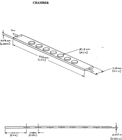
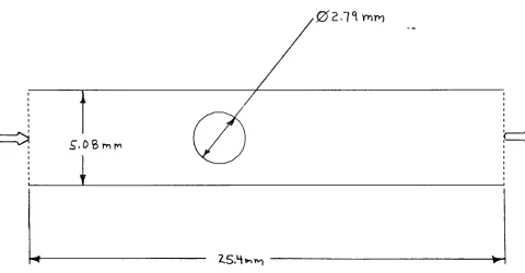
applications.

Figure 1-1

shows a

typical

channel

for

apolymerasechainreaction

(PCR)

detection

chamber.

PCR is

a method of

DNA

analysis

that

requires

fluid flow

over

detection

probes

in

an

enclosed space.

Figure 1-1 has dimensions

that

aremuch

larger in

the

width

(W)

direction

than

in

the

height

(H)

direction. The

small size of

the

channel results

in Reynolds Numbers

that

are

very low (Re

<

5). This low Reynolds's

numbermeansthat

the

flow

will

become

fully

developed in

a

very

short

length

comparedtothe overall channel

length.

The low Reynolds Number

and

the

geometry

of

W H

lead

to this

fluid flow

being

a

variation oftwo

types

of common

families

of

flow

problems.

Stokes Flow: Applicable

with

very

small

Reynolds

number.

When

thisoccurs

the

viscous

forces

overwhelmthe

inertia

forces. This

allows the non-linear

terms

in

the

Navier Stokes

equations

to

be

neglected.

Hele-Shaw

Flow: Involves

slow

flow

ofa

fluid between

parallel

flat

plates which are

fixed

at a small

distance

(H)

apart.

Hele-Shaw flow is

often created

in

experimental

test

configurations

to

help

understand

the

basic flow

phenomena.

Stokes flow is

often assumed

because

thisallows

the

full

Navier-Stokes

equations

to

be

simplified

to the

point where

they

can

be

solved

for

specific

configurationsand

boundary

conditions.

These

flow

types

are

very

useful

for

understanding

some

fluid flow

configurations.

However,

the

assumptions required

limit

their

usefulness

to

Using

computational

fluid dynamics

(CFD)

codes

to

solve

these types

ofproblems allowsa

person

to

examine a wide range of

geometries,

boundary

conditions,

and

fluid

types

in

a

time

effective manner without

the

expense of a good experimental

test

set-up.

Over

the

last

decade CFD

solution

techniques

have

improved both in

computational

efficiency

and numerical accuracy.

Also

computing

hardware has

advancedto thepoint where

individual

engineers and scientist

have

attheir

disposable relatively low

cost

workstationsthatare capableof

analyzing

complex

fluid flow

problems

in

reasonabletime

periods.

These

advances

have led

to the

development

ofnumerous

commercially

available

CFD

software codes.

FLUENT from

Creare,

Inc. is

one ofthesecommercial

CFD

codes.

The

software

includes both

pre-_and

post-processing capability

thatallowthe

flow geometry

to

be

created and modified as required.

This

allows a wide rangeofvariables

to

be

modified

to

Figure

1-1

TYPICAL

CHANNEL GEOMETRY

FOR

PCR

DETECTION

CHAMBER

O.OTt.mm

(o.

003>!>0

jzte.8 tvi^

(01.1

in)

(O.Z ir>)

-lO.lfepiM--H S.06mtn

(O.ZtJi*')

0.02.^mrvi [image:16.557.33.515.85.637.2]

1.1

APPLICABILITY

OF HELE-SHAW

FLOW

Hele-Shaw

(1898)

used an experimental set

up

to

determine

the

streamlines

for

the

flow

around

bodies

of

arbitrary

shape.

He

showed

that

a three-dimensional viscous

flow

between

two

closely

spaced

flat

plates exhibited

two

dimensional

potential

flow

patterns.

Figure

1-2,

from 'Viscous

Flows'

by

Ockendon

and

Ockendon

(1995)

showsa

typical

Hele-Shaw

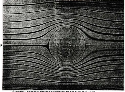
cell.

Figure

1-3,

from 'Visualized

Flow'

compiled

by

Nakayama

(1988)

shows

the

flow

patternthatresults when

looking

down

atthe

top

ofthe

Hele-Shaw

cell.

There

aretwoaspects of

this

study

that

fall

underthegeneral

Hele-Shaw flow

analogies.

The first

aspect ofthe

Hele-Shaw flow is

that

for

themotion ofa viscous

fluid,

between

two

fixed

parallel plates which are

sufficiently

close

together,

Saffman

and

Taylor

(1958),

define

the

mean

velocity in

the

cell as

follows.

b2

(dp

u=-T27bi+pg|

(L1)

b2

dp

v =

The

second part of

the

Hele-Shaw analogy

that

is

applicable

to

narrowchannel

flow is

when

one

fluid

of a

different

density

is

acceleratedperpendicular

to

the

interface

of another

fluid.

This

is

thecase when one

fluid is

at rest

in

thechannel andanother

fluid is

pushed

into

the

channel

to

"wash

out"

theprevious

fluid. When

the

accelerating

fluid

has

the

higher

density

the

interface between

the two

will

be

stable.

When

the

less

dense fluid

is

accelerated

into

the

higher

density

fluid

the

interface

will

be

unstable,

Saffman

and

Taylor

(1958).

The

typeof

fluid

flow

that

will

be

studied

in

thiscase will

be

avariationofthe

Hele-Shaw

flow.

For Hele-Shaw flow

analysis,

any

obstruction

in

the

channel

is

assumed

to

take

up

the

complete

height. This study

will

look

at cases wherethecylindrical

disk

obstructions are

less

than

the

height

ofthechannel.

The

second extension of

Hele-Shaw flow

thatwill

be investigated is

the

interaction

between

thecylindrical

disk

andthe sidewalledges.

Pure Hele-Shaw

cells assumethat the

flow

around

any

obstructions arenoteffected

by

side walls.

The

abovetwoextensionsof

Hele-Shaw flow

can

be

thought

of as

taking

the

Hele-Shaw

flow

which

is based

on

the

flow

being

analyzed

in 2-dimensions

and

extending

the analysis

Figure 1-2

TYPICAL HELE-SHAW

GEOMETRY

Hele-Shaw

flow

Figure

1-3

FLUID

FLOW

PATTERN

FOR

HELE-SHAW

CELL

[image:20.557.69.488.203.512.2]

1.2

APPLICATIONS

1.2.1 POLYMERASE CHAIN

REACTION DETECTION POUCH

This

study

was undertaken as an attempt

to

understandtheperformanceof

PCR detection

pouches.

The

polymerase chain reaction process

(PCR)

is

a method

for amplifying

and

capturing

specific samples of

DNA. PCR

amplification

may

contain

6

x

1011

copies of a

particular

DNA

targetstrand.

One PCR detection

method

described

by Findlay

et al

(1993)

combines

the

amplification and

detection

process

in

a single closed vessel.

The detection

process relies onthe specific

hybridization

tooligonucleotide probes and enzymatic signal

generation.

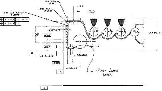
Figure 1-4

shows a

drawing

ofthe

PCR

'pouch' used

for

thisprocess.

The PCR

pouch shown

is

an expandable plastic

design. To

analyze

the

flow in

thenarrow

detection

chamberthechannel

geometry

will

be

approximated as a rigid rectangularchannel.

The detection

process works after

hybridization,

when

biotinylated PCR

products are

capturedonthe

discrete detection

spotswherever

they

encounterprobes

complimentary

to

theirsequence.

After

subsequent

treatment

with

different fluids (streptavidin-horseradish

peroxidase

conjugate,

wash

solution,

and

dye

precursor

solution)

colorwill

develop

onthe

detection

probes

One

ofthegoals

in

the

design

ofthis

PCR

pouchwastominimize

the

amount of

fluids

requiredto

carry

outtheprocess.

The

second goalwasto

be

able

to

determine

a positive or

negative

test

result

by

visual comparison of

the

detection

probes against a color chart or

instrumentally

by

reflection

densitometry. The

combinationof

the

two

previously

mentioned

goalsmeans

that the

fluid flow

acrossthe

detection

probes

is

critical

to the

performance of

The 'color

response of

the

detection

probe

is

based

on

diffusion

from

the

fluid

to the

probe

and

the

process

is

sensitive

to

sample concentration

in

the

fluid

and

the

probe.

The

process

is

rate sensitive which

leads

to the

importance

ofwell understood

fluid

andthermal

boundary

conditions.

1.2.2 OTHER

APPLICATIONS

Other

types

of

fluid flow

where

this

analysis

for flow in

narrow channels withobstructions

could

be

applicable are as

follows.

1. Blood flow

with

blockage;

the

flow

of

blood

in

the

body

throughnarrow arteries or

veinswithsome

type

of

blockage

would

fall into

thisgeneraltypeof application.

The

geometry

of

the

rectangular channel andcylindrical

disk

blocking

the

fluid flow

would

be

modified

for

this

analysis.

2. Flow

of

fluid in Ink Jet

printer;

Inkjet

printers requirethe

flow

of

fluid in

narrow

channels.

Also

the

insertion

of

cleaning

fluids

or

different

color

inks

could

fall into

Hele-Shaw

flow

depending

on

the

geometry

ofthe

flow

path.

3.

Electronic cooling in

micro-channels;

small electronic systems such as

multi-chip

modulesoften require goodthermalcontroltomaintain accurate performance.

This

can require

fluid

flow

oversmallelectronic components

to

remove

the

power

being

Figure

1-4

PCR

Detection

Pouch

.110 DIA .OIO'

7 DOTS

?

0.050% A B C

4- ₀

.030% A

[image:23.557.15.540.225.520.2]

!-3

PROBLEM

_DEFINITION

The

PCR detection

_process

is

based

on

getting

positive or negative readings on each

detection

probe. Positive

readingsare obtainedwhen

the

fluid

passing

over

the

detection

probe

diffuses

sufficientamountsof

the

DNA

strands,

wash

fluid,

and

dye fluid

into

the

probe.

The

diffusion

process

depends

on

the

sample concentration

in

the

detection

probe and

in

the

fluid passing

through

the

detection

chamber.

The

ratethe

fluid

passes overthe

detection

probe andthepressure

the

fluid

exerts on

the

probe are significant

factors in

obtaining satisfactory

machine performance.

Experimentally

determining

the

flow

rateand pressure

is

not an

easy

process given

the

miniature

geometry

of

the

PCR

detection

chamber.

Using

CFD

tools

to

analytically

determine

the

flow

field

is

a

lower

cost approach

in

termsof

time,

people,

and money.

Figure 1-5

shows a cross section ofthe

detection

chamber

inside

the

PCR instrument. This is

the

geometry

as the

fluid is passing

through

the

detection

chamber.

The PCR

pouch

is

nominally flat

and expands as

fluid

passesthroughthe

detection

chamber.

The

analysis ofthis

type

of

fluid

problem requires

the

definition

of several variables.

These

include

the

following.

1.

Geometry

Configuration

2.

Fluid

type

3.

Fluid

properties

4.

Boundary

conditions

Inlet flow

rate or

velocity

Outlet

conditions

Wall

properties

Figure 1-5

PCR DETECTION CHAMBER GAP

CROSS SECTION

Fixed

@

+/-.002"

Detection)

Pfc.og,E

The

overall

geometry

size was

previously

shown

in Figure 1-1. This

shows

the

problem

to

be

a

full 3-dimensional

problem.

This

work will approachtheproblem

in 3-D because

diffusion

into

the

detection

probes

depends

on

flow

on

both

the

top

and side walls.

The length

of

the

detection

chamber and

the

numberof

detection

probes will

be

reduced

to

minimize

the

computationaltime.

The 3-D

solution will

be

reduced

to

25.4

mm and

the

number of

detection

probes will

be

reduced

to

2. This

reduction

in geometry

size will

greatly

reduce

the

problem run

time

and still allow

the

effect of probe andchamber

geometry

on

the

flow field

to

be determined.

The

typeof

fluid

will

be

assumed

to

be

water

for

all cases.

The

actual

PCR

processuses

several

different

fluids

but

they

allare

largely

water

based.

Using

wateralso means

the

fluid

properties are

readily

available

in

standard publications.

The

inlet

boundary

conditions

for

thiswork will use a nominal

inlet velocity

of

0.01

m/sec

in

mostcases.

This velocity is based

ontheamount of

fluid in

the

PCR

pouch andexperimental

results

for

the

time

it

takes

the

fluid

to transverse

the

length

ofthe

detection

chamber.

The

outlet

boundary

conditions

for

theactual

PCR

pouchconsist of a

large

fluid

reservoir.

The

outlet ofthe

detection

chamber will

be

approximated as an

infinite

reservoir.

The

walls and

the

detection

probeswill

both have

a

'no

slip'

boundary

condition applied

during

the solution of

this

problem.

In

actual practice

the

detection

probes are porous cells.

Experimental

results

have

shown

this to

be

a

secondary

effect on

the

fluid flow

within

the

This

problem will

be

solved

using

the

CFD

software code

FLUENT.

The

problem will

be

solved as a

steady

state solution.

Given

the

finite

amount of

fluid in

the

PCR

pouch, this

steady

state solution would

only be

valid

for

a

very

short amount oftime.

However,

the

steady

state solution will provide excellent

insight into

the

flow velocity

andpressure

distribution

within

the

detection

chamber.

1.4

OBJECTIVES

OF THE PRESENT WORK

The

objectives of

this

work are given

below. These

objectives are

based

on

the

desire

to

have

uniform

flow

over

the

maximumpossible surface areaofthe

detection

probes

in

the

PCR

process.

This

is because

thechemical reaction

between

the

DNA

strandsandthe

detection

probes

is

a rate

dependent diffusion

process

that

depends

on

the

concentration of

species

in

the

fluid

and

the

detection

probe.

These

objectives are

based

on

first verifying

that

FLUENT

is

a propertool

for analyzing

this

type

of

flow

problem andthen

using FLUENT

to analyzethe

full 3-D flow field.

1

.

Compare

the results

from

potential

flow

theory

to

FLUENT

for flow

over cylinders.

2.

Compare

the

FLUENT

resultsto other published results

for flow

over a cylinder.

3.

Determine if FLUENT

will

properly

predict

the

effect of walls

located in

close

proximity

toa cylinder.

Use

thepotential

flow Method

of

Images

theory

for

verifying

the

FLUENT

results.

4.

To

show

that

commercial

CFD

codes such as

FLUENT

can

be

used

to

analyze the

three

dimensional fluid flow in

narrowchannels

approximately 0.04

mm

thick.

5.

Determine

thepressure

distribution

on

the

detection

probes

for

a

typical

geometry.

2.

LITERATURE

REVIEW

There

is

no

literature

available

to

the author's

knowledge

on a

detailed study for 3-D fluid

flow

around cylinders within a rectangular

duct. There is however

a

large

body

ofwork

for

simplified versions of

this

problem.

The

case of

two

dimensional

fluid flow

arounda

cylinder

is

a

very

popular

test

case

for verifying different CFD

codes.

The American

Society

of

Mechanical Engineers

published a compilation(FED-

Vol.

160)

of

different

papers

from different CFD

vendors with solutions

to the

2-D

cylinder

flow

problem.

All

ofthesepapers were presented atthe

Fluids

Engineering

Conference

in 1993.

The

paper

by

Kim

and

Choudhury

(1993)

is

of particular

interest

as

it

employsthesame

software,

FLUENT,

which

is

used

in

the

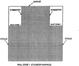
current study.

Kim

and

Choudhury

(1993)

use a unique grid structurethat

is

a combinationof

O-type

grids

aroundthecylinder and

hexagon

grids

far

upstream and

downstream from

the

cylinder.

This

grid structure

is

shown

in Figure 2-1. This

grid structure

is

effective

for getting

good results

aroundthecylinder

using

the

O-grid

and also

far

afield

from

thecylinder

using

the

hexagon

grid.

A

key

simplifying

assumption made

in

this

paper

is

the

assumption

that

a

'free

stream'

boundary

condition

is

usedtosimulate

the

walls

surrounding

the

flow. The free

stream

boundary

condition

implies

that thestream

function is

equalto zero and also

the

vorticity is

equal

to

zero.

Kim

and

Choudhury

accomplish

this

by

setting

the

outer walls as

symmetry

boundaries. The

assumptionof

free

stream

boundary

conditions are

designed

to

have

the

effect of

removing

the

wall

from

the

solution.

Depending

on

the

numerical approach

used,

different

authors use

different

techniques to

approach a

free

stream

boundary

condition at

the

Figure

2-1

O-H Grid

Structure

used

by

Kim

and

Choudhury (1990)

CYCLIC

SYMMETRY

INLET ZONE 1

/

OUTLET

/

SYMMETRY

INLETZONE 1

CYCLIC

WALL ZONE1 (CYLINDER

SURFACE)

Computational

Grid

SYMMETRY

OUTLET

[image:29.557.132.434.159.410.2]

Kim

and

Choudhury

(1993)

state

that

in

the

vicinity

of

Recyi

=

5,

the

flow

starts

to

separate

to

form

a pair of

recirculating

eddies attached

to

the

body.

They

also state

the

eddies

formed

behind

the

cylinder remain

stationary

until another

bifurcation

takesplace around

Recyi

=

40.

Beyond

Recyi

=

40,

the

flow

becomes

_{asymmetric and}

unsteady,

being

accompanied

by

alternate vortex shedding.

Kim

and

Choudhury

(1993)

present alloftheirresults

based

on

Recyi

=

60.

For

the work presented

in

this

reportthe

Recyi

will

be

equal

to

42

or

less. The

Recyi

approximately

equal

to

40

was chosen

because

it

represents

the

actual

flow

rate

for

the

PCR

process.

Unfortunately

this

is

the

Reynolds

number

that

is

the

dividing

point

between steady

flow

and

unsteady flow

caused

by

vortex shedding.

The

results

described

by

Kim

and

Choudhury

(1993)

are consistentwithexperimental results

available

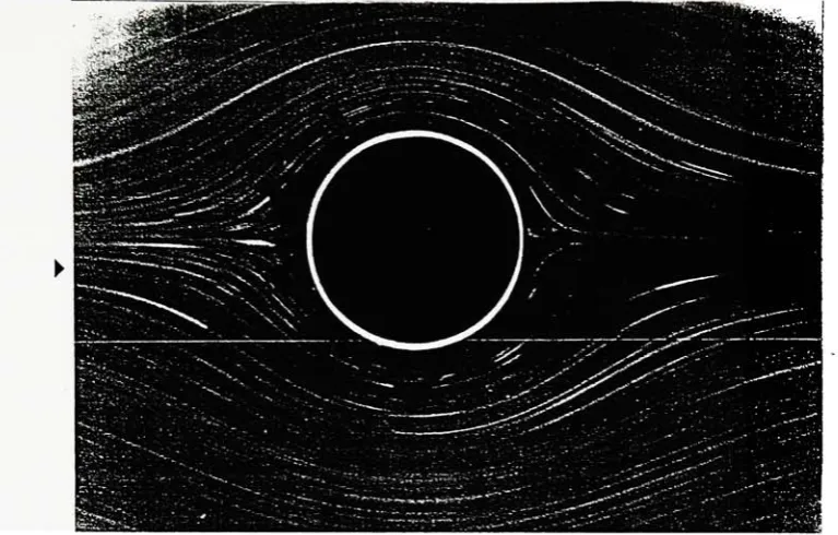
in literature. Shown in Figure 2-2

are some

flow

experimental

flow

results

from

Nakayama

(1988)

for very low Reynolds

numbers of

less

than

2. Notice

that

there

are no

eddies onthe

back

side of

the

cylinder.

As

the

Reynolds

number

is increased

theeddies

do

begin

to

form. Figure 2-3

shows some

moreexperimental results

for Nakayama

(1988)

for Reynolds

numbers of

16

and

26. Once

the

Reynolds

number

is

increased higher

the eddies

become

unstable and

begin

to

shed.

Figure

2-3

also shows anotherexperimental result

for Nakayama

with a

Reynolds

number of

55. At

thispointtheeddies arenotattachedtothe

back

of

the cylinder,

andthe

flow is

now

[image:31.557.91.475.136.381.2]

Figure 2-2

Experimental Flow

Pattern

for

Low

Reynolds

Number

Flowaround a circularcylinderatRe=_0.038

(glycerine,

_{flow velocity0.15}

cm/s,

cylinderdiameter 1.0 cm,tankwidth40cm,aluminium powder method).

[image:32.557.61.497.313.579.2]

Figure 2-3

Experimental

Flow Pattern

at

Reynolds Numbers

of

19, 26,

and

55

Flow

around acircular cylinderat

Re

= ₁

9

(water,

flow

velocity

0.20

cm/s,cylinder

diameter

1.0 cm, aluminium powder

method and electrolytic precipitation

method).

Flow

around acircularcylinder at

Re

Flow

around a circular cylinder at

Re

=

26

(water,

flow velocity 0.25

_cm/s,cylinder =

55

(water,

flow velocity 0.55

_{cm/s,cylinder}

diameter

1.0

cm, aluminium powder

diameter

1.0

cm, aluminium powder

The

numericalresults

from

this

analysis will

be

compared

to the

resultsof

Braza

etal.

(1986),

Dennis

and

Chang

(1970),

and

Fornberg

(1980). All

these

papers

because

of

simplifying

boundary

conditions on

the

walls

base

the

Reynolds

number on

the

cylinder

diameter

rather

than the

channel geometry.

Dennis

and

Chang

(1970)

solved

the

2-D flow

problem

for

5

<

Recyi< 100 using

a

finite

difference

solution

technique.

Dennis

and

Chang

(1970)

also

apply

the

free

stream

boundary

condition at

the

wall.

They

do discuss

other possible

boundary

conditions

but do

not give

any

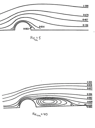
results.

Figure 2-4

showsthestream

line

plots

from Dennis

and

Chang

(1970)

for

Recyi

equal

to

5

and

40. Notice

the

difference

in

the

flow

pattern

behind

the

cylinder.

The

Recyi

=

40

_plot

clearly

showsthe

circulating eddy

that

were

previously discussed. This

eddy

does

not occur

for

the

lower

Recyi

.

The

other portionof

the

Dennis

and

Chang's

(1970)

result

that

is

of

interest is

the

results

from

the

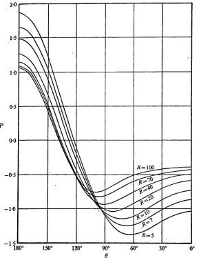
pressure coefficient onthecylinder surface.

Dennis

and

Chang

(1970)

define

a

dimensionless

pressure coefficient given

in

equation

2-1

.

Figure 2-5

shows

the

result of

this

pressure coefficient

for different Reynolds

numbers.

Figure

2-4

STREAMLINES

FOR

STEADY

FLOW

PAST A CIRCULAR

CYLINDER

FOR

Re

=

5 AND 40

,

Dennis

and

Chang (1970)

c-n.

1-223

[image:34.557.141.468.165.605.2]

Figure

2-5

DIMENSIONLESS

PRESSURE

COEFFICIENT ON THE CYLINDER

SURFACE,

Dennis

and

Chang (1970)

20

1-5

10

0-5

00

-0-5

-10

-1-5

180'

^

\

i

%

\|

.R=100___

^

(^

150 120 90

e

[image:35.557.140.429.178.552.2]

Fornberg

(1980)

analyzedthe

flow

over

the

cylinder

in

a similarmethod

to

Dennis

and

Change

(1970). The

main

difference

is

Fornberg

(1980)

places much greater emphasis on

the

types

of

boundary

conditions

to

apply.

He

points out

the

calculations

for vorticity

around

the

cylinder can

have

an error

in

excess of

20%

when

using

a

free

stream

boundary

condition.

This

is

true

even

if

the

boundary

condition

is

applied

far away (23

times the

radius) from

the

cylinder

body.

Fornberg

considers

four different

boundary

conditions.

1

.

Free

stream

2.

One

term

ofthe

Oseen

approximation

3.

Normal

derivative

of stream

function

=

0

4.

A

mixed condition of option

1

and

3

The

free

streamcondition

implies

that

thestream

function

equals

0

at

the

wall.

This

will

neglecttheeffectofthe

boundary

layer

onthewall.

Combining

thiswith

the

gradient

being

zero

does

not

fully

take

into

accountthe wall effect.

To

get the

full

walleffect one needs

to

make the actual

velocity

equaltozeroand allowthe

boundary

layer

atthewallto

form.

Fornberg

presents results

very

similar

to

Dennis

and

Chang

(1970)

for

stream

line

and

vorticity.

The

paperpresentsresults

for 2

<

Recyi< 300.

A different

solutionmethod

is

used

for Reynolds

numbers

less

than

10,

but

no

details

are given onthis solution method except that

it

is

based

ona

fast Poisson

solver.

The

reportof

Braza

et al.

(1986)

compares

the

numerical results

to

experimental results

from

different

authors.

The

solution methodused

is

similarto

FLUENT

in

that the

governing

equations arewritten

in

avelocity-pressure

formulation

and

in

conservative

form,

are solved

by

apredictor-correctorpressure

method,

a

finite

volume second order accurate scheme and

Braza

(1980)

also uses a

finite

volume

technique

(the

sameas

FLUENT)

instead

of a straight

finite

difference

technique

like Dennis

and

Chang

(1970). Braza

statesthat

the

governing

equations

integrated

over an

elementary

control volume enhance

the

local

mass

andmomentumconservation near

the

boundaries

better

thana simple

finite

difference

approximation scheme.

Braza

(1980)

also rewrites

the

governing

equations and solves

them

in

a

logarithmic-polar

coordinate system.

This

makes

the

gridconfigurationconformcloser

to the

cylinder geometry.

The

results of

Braza

et al.

(1980)

show a greater negative pressure coefficientthan

the

results of

Dennis

and

Chang

(1970). For

a

Reynolds

numberof

40,

Braza

etal.

(1980)

have

a minimum value of-1.19where

Dennis

and

Chang

(1970)

have

a minimum value of-0.95.

Braza

et al.

(1980)

does

give a

different definition for

the

pressure coefficient

Cp

than

Dennis

and

Chang

(1970). It is believed

by

this

authorthat

Braza's

definition is

a

typographic

mistake

because

the

results presented agree well withother published results.

Using

Braza's

definition

as published wouldresult

in significantly different

results.

One

ofthereasons

for

the

different

results

between Braza

et al. and

Dennis

and

Chang

is

because

they

each use

slightly different

governing

equations

to

define

the

flow field.

Braza

et al.

have

writtenthe

governing Navier-Stokes

equations

in

terms

ofpressure and

velocity.

Dennis

and

Chang

have

simplifiedthe

governing flow

equations and written

the

equations

in

termsofstream

function

andvorticity.

Extensive

use was also madethroughoutthisreportof

the

classic

books

that

have been

2.1

BASIC

GOVERNING

EQUATIONS

The

following

section presents some ofthe

top

level

governing

equations.

These

equations

can

be found in

one

form

or another

in

standard

fluid

mechanics

text

books. The

following

discussion

will

include

both

real

fluids

with

viscosity,

and no

slip

at

the

solid

surface,

along

with

ideal flow

wherethe

flow is

allowed

to

slip

and

the

viscosity is

assumed zero or

neglected.

Most

of

the

theory

summarized

here

wascontained

in books

by Schlichting

(1979),

Churchill

(1988)

and

Fox

and

McDonald

(1985).

2.1.1

FLUID FLOW GOVERNING EQUATIONS

Given in Figure 1-1 is

the

geometry for

the

PCR

detection

chamber.

The

small size ofthe

chamber and

the

minimal amounts of

fluid

meanthat

the

Reynolds

numberwillalways

be

very low

.

Re

=

p_ULc

(2.2)

M-For

the

geometry

ofthe

PCR

detection

chamberthecharacteristic

length is

the

hydraulic

diameter.

Lc=Dh=4Ac

(2.3)

P

Most

ofthepublished

literature

concentratesonthe

flow

around

the

cylinder and

simplifying

the

wall

boundary

conditions.

For

this reason

the

characteristic

length

used

in

the

published

data

is

the

cylinder

diameter. In

thisreport

the

Reynolds

number

based

on

the

cylinder will

The Navier Stokes

equations and

the

conservationof mass

(or

continuity)

equation

that

define fluid flow in

the

detection

chamber areas

follows

continuity:

3p_

+

V(pu)

=

0

(2.4)

3t

pDu =

-Vp

+ |iV2u

(2.5)

Dt

Where

D

d

d

d

d

= ₊u- ₊v₊w

(2.6)

Dt

dt

dx

dy

dz

V=i+J_+k

(2.7)

dx

dy

dz

u = _{i +}

vj

+ wk

(2.8)

This form

ofthe

Navier-Stokes

equation assumes

incompressible flow

and variations

in

the

fluid viscosity

can

be

neglected.

Both

of

these

assumptions are valid

for

the

analysis

in

the

PCR detection

chamber

because

the

flow velocity is very low

and

the

chamber

is

held

at a

constanttemperature.

In

the

case of

frictionless

flow,

where

the

viscosity

is low

and can

be

neglected

([J.

=

0),

the

Navier-Stokes

equationcan

be

reduced

to

Euler's Equation.

Du

_

p =_pg-V/>

Even

though

all real

fluids have

viscosity, there

is

a significant amount ofpublishedwork on

ideal fluid flow.

Flow

with zero

viscosity

is defined

as

inviscid fluid

flow. There

are no

shear stresses present

in

inviscid

fluid

flow.

2.1.2 POTENTIAL FLOW

For

classical potential

flow

theory,

the

flow

must

be both inviscid (fi

=

0)

and

irrotational.

The

key

assumption

in

this type

of

flow is

that

fluid friction

nearthe

boundary

can

be

neglected.

In

real

fluids

this

is

never

true, but

potential

flow

can give acceptable

understanding

of

the

flow

phenomena provided you

do

not

look

too

close

to

the

boundary

wall.

Potential flow

analysis

is

a

very

populartechnique

because

thereare a

large

number of

analytical solutions

representing different

types

of

fluid

flow. Potential flow

analysis

is

currently

being

used

to

help

in

the

design

of

airplanes,

boats,

and automobiles.

There is

a

large

body

of work

that

falls

underthe

heading

of

Potential Flow. This

report will

concentrate on

only

two

dimensional

potential

flow. In

two

dimensions,

with constant

density,

the

conservation ofmass given

in

equation

2.4

reduces

to

the

following.

+

-0

(2.10,

dx

dy

The

stream

function

is defined

suchthat

it

also satisfies

the

continuity

equation.

u=

(2.11)

3y

v=

The

same

continuity

equation and stream

function

can

be

defined in

cylindricalcoordinates.

This

will

be

very

useful

for

looking

at

flow

around acylinder.

drV

dV

Conservation

of mass: + - =

₀

(2.

13)

dr

dd

Stream

function:

V=-^-

(2.14)

r

dO

Ve=-d-l

dr

(2.15)

To be

a potential

flow

the

flow

must

be both inviscid

and

irrotational. For irrotational flow it

is

possibleto

define

a

velocity

potential as

follows.

V

=-VO>

(2.16)

The

above

definition

for

the

velocity

potential

is

notconsistent across

different fluid

text

books.

Many

sources

define V

=

V<E>

.

This

report will use equation

2.16

because it leads

to

thepositive

direction

of

flow

being

in

the

direction

of

decreasing

potential.

In

cylindrical

coordinatesthe

velocity

potentials are

define

as

follows.

d

Vr=~

(2.17)

dr

For irrotational flow

the

fluid

elements

in

the

flow field do

not undergo

any

rotation.

This

leads

to the

following

equation

for

an

irrotational flow.

^-^

=

₀

(2.19)

dx

dy

Substituting

the

definition

for

the

stream

function (eq. 2. 1 1

and

2.12)

into

the

irrotational

flow

equation

(2.19),

and

substituting

the

velocity

potentialequation

(2.16)

into

the

continuity

equation

(2.10)

it is

possibletoobtain

two

equationsthatare

both forms

of

Laplace's

equation.

Also any function *P

or

O

that

satisfies

Laplace's

equationrepresentsa

possible

two-dimensional,

incompressible,

irrotational flow field.

t

+

^-T

=

(2-2)

3x2 3y2

<92<D (920

^+^=

<221)

Part

ofthereason potential

flow

analysis

is

so oftenused

is

that

different elementary flow

patterns can

be

added

to

one anothertocreate a complex

flow

pattern.

Both

<1>

(velocity

potential)

and

*F (stream

function)

satisfy Laplace's

equation

for flow

that

is

incompressible

and

irrotational. Since Laplace

equation

is

linear

and

homogeneous

partial

differential

equation solutions

may be

added

together.

Using

superposition

it

is

possible

to

simulate

the

flow

around

the

cylinderandthewalls

for inviscid

flow.

Superposition

can

be

used

because

each potential

(O3

=

Oi

₊

O2)

is

_{a unique solution of}

Laplace's

equation,

V2<P

=

0. To

_create

flow

around a

cylinder,

superposition

is

used

for

uniform

flow

past a

doublet. A doublet is

a

combinationofa source and sink

ideal flow. Figure 2-6

shows

the

flow

configuration

for

a

Figure

2-6

UNIFORM

FLOW

AROUND

A

CYLINDER

--LL

_oO

r-a

Uniform

Flow;

velocity

potential

stream

function

O

=-Ux =-U^rcosO

(2.22)

(2.23)

Doublet;

velocity

potential <D=

-Acos0

(2.24)

stream

function

*F

=

-Asin0

(2.25)

Cylinder;

^cyl

=

^uniform

₊

^doublet

(2.26)

= _{U rcosd}

-Acosfl

(2.27)

Any

closed streamlinecan

be

takenasthe surface of a solid

immersed in

the

fluid flow. This

means

the

cylinderwall

is

represented

by

the

streamline

*F

=

0. For

_the

inviscid flow

_around

acircular cylinderwithradius=

a,

andA=

U^a2

,

Churchill

(1988)

gives

the

following

equations

for

thepotential

functions

and stream

functions in

cylindrical and rectangular

coordinates.

0

=-u

' a2^

r+

K

r J

,2

A

cost?=

-ux\

1

+ ₂ , 2

x

+y

)

(2.28)

T

=

-uM

(

a2^ r

^

r

J

(

sin=

-uy

,2

>

1

+

2 . 2

The

velocity

components

in

cylindrical coordinates are

1

dy/

. a

ur

= -- =

U,

r

d6

'l-^lcosfl

(2.30)

V

6

dr

fi

2)

V r

J

sing

(2.31)

The velocity

at

the

surface r=_a

is

_then

"e,fl=-2LLsin0

(2-32)

u =

₀

(2.33)

The velocity is

seen

to

be

zero atthe

forward (0

=

7t)

andrear

(0

=

0),

_{whichare calledthe}

points ofstagnation.

The

pressure

distribution is

given as

Pa=P+

^=- [1-4

sin2

d]

(2.34)

The

previous equations

have

defined how

topredict an

ideal fluid flow for

uniform

flow

around acylinder.

These

equations

do

nottake

into

account

any

effect walls outside

the

cylinderwould

have

onthe

flow. To

create

the

walls

the

method of

images

can

be

used.

"The

methodof

images

was

introduced

by

Kelvin

for

use

in electricity

and

later

used

by

Helmholtz

and

Stokes in fluid

dynamics."

Granger

(1975)

To

model uniform

flow

over a cylinder

between

two

walls requires

that the

singularity inside

the walls,

which will

be

the

same

ideal flow doublet

thatwas

previously

discussed,

the

doublet

will

have

to

be

reflected outside

the

walls.

Note

that to

fully

accomplish

this

each

reflectionwill

have

to

be

reflected

itself,

whichmakes

the

final

solutiona series of

reflections.

Figure

2.7

shows arepresentation of

the

reflected

doublet. The

cylinder

is

defined

the

same as

in

the

previous section

by letting

the

cylinder radius

be

the

point where

the

stream

function

is

equal

to

zero.

Chung

(1978)

gives

the

stream

function

and

horizontal

velocity using

themethod of

images

as

follows.

=

/_

?-hr-H

lit

sinh'

(id>\

.

(2jty

sin

-\H)

V

H

H

,2i

nx)

i(

xy

cosh cos '

H

(2.35)

The velocity is determined

by

taking

the

derivative

of

the

stream

function.

d*F

Vx

=

^r-

=

U.

x

dy

1-sinh'

Kb^

(2iiy

cos -cosh'

^KX^

VH;

-cos

^7ty^

+

-2

{Hj

sm

'27cy

cosh'TtX

h".

cos 'icy"

(2.36)

vy

=

-dx

2

"

Ih,

sin

-sinh

I

H

J

I

H

J

cosh2

Ih

-cos

2f

ny

H

A

nice aspect of potential

flow

is

that

after

determining

the stream

function

and

then

taking

the

derivatives

to

get

the velocity, the

velocities can

be input

into

Bernoulli's

equation

to

get

the

pressureprofile.

Zj_

+

ghi

+

PL

=^L₊

gh2

+

P^

(2.38)

2

P

2

p

The

flows

thatwill

be

discussed

in

this

report will

have

negligible change

in

elevation

(h)

and will also

have

constant

density. Also

on

the

cylindrical surface

the

radial

velocity is

zero.

Pcy,=P~+^(ui-Ue2)

(2.39)

The

above equationcan

be

rearrangedtoput

it in

thesame

form

as equation

2. 1

which

defines

thenon-dimensional pressure coefficient.

Figure

2-7

DOUBLET

REFLECTED

USING

METHOD

OF

IMAGES

///'//

^-t

/

/

H

3.

THEORETICAL ANALYSIS

3.1 FLUID FLOW IN RECTANGULAR DUCTS

The

solution

for

the

axial

velocity

(u)

for

fully

developed laminar

three

dimensional

flow in

a rectangular

duct is

as

follows.

u =

16Cia2

n~

:1-\ s n

2

n=l,3,5

cosh

1

2a

cosh nKb

2a

cos

(

_nnz^

V

2a

j

(3.1)

For

the above equation

C\

is

a

function

ofthepressure

drop

andtheviscosity.

Shah

and

London

(1978)

give

the

equation

for

the

mean

velocity

(Um)

related

to

Q

as

follows.

Ci=

3

Ur

7t5

UJil..n5

I

2a

-1

2a

j

(3-2)

The

results oftheabove equationshowthat

flow in height direction

(H)

direction is very

much

like

the

flow between

two

parallel plates.

Figure 3.1 is

a plot of

the

velocity

profile

Figure 3-1

VELOCITY

PROFILE

ACROSS GAP

HEIGHT

n =1,3..

19

C,:=l z:=0.0 a:=l b:=l

0.5

ys

o

-0.5

\

\

\

\

\

\

1

J

/

\

-^

^"

0

0.05

0.1

0.15

0.2

0.25

0.3

Looking

at the

top

of

the channel,

across

the width, the

flow

maintainsauniform

velocity

except nearthewalls.

This

result gives an

understanding

of

why

the

Hele-Shaw

cell

previously discussed

works

very

well

for simulating ideal flow in

two

dimensions. Except

for

a small

boundary

layer

near

the edge, the

flow velocity looks very

much

like ideal flow.

Figure

3-2

shows a plot

looking

down

on

the

top

oftherectangular

duct.

Figure 3-2

representsthe

flow

looking

atthe

top

of

the cell,

orthe

velocity

gradientacross

the

width.

The flow looks exactly like inviscid irrotational flow in

two

dimensions (2-D slug

flow),

if

the

edge effectsnear

the

walls are neglected.

This

means we can treat

the

flow

as

ideal flow

and use potential equations

to

model

flow

around

any

objects

located in

this

area.

This

type

of

flow has been

analyzed

experimentally

by

theuseof

Hele-Shaw

cells.

The

flow

field for

a

Hele-Shaw

cell can

be

shown

to

satisfy

the

Laplace

equation.

When

a cylindricalobject

is

placed

in

the

gap

of a

Hele-Shaw

cell,

theequations showthat

themean

velocity is

thegradient of a potential

function. This

meansthe

flow field

pastthe

Figure 3-2

FLUID VELOCITY ACROSS

GAP WIDTH

n =1,3..199 _y :=

0 a- 0.00254

m b:=3.8098 10

Um=0.01m/s

0.002

z.

l

0

0.002

______-_._____-__-___-.

0

0.005

0.01

0.015

0.02

3.2 INVISCID IRROTATIONAL FLOW IN TWO

DIMENSIONAL FLOW

This

section will present

the

solution

for

the two

dimensional flow

witha cylindrical

obstruction.

The

two

dimensional

flow

field

will

be

solved

in

acoupleof

different

methods.

1.

2-D

potential

flow

without walls

2.

2-D

potential

flow using

the method of

images

to

simulate walls

Method

1,

2-D

potential

flow

without walls willsimulate

the

uniform

flow

arounda cylinder

thatwas

discussed in

section

2.1.2. Method 2

will

determine

theeffectof

adding

thewalls.

There

will

be

threeaspects ofthe

flow

solutionthat will

be important.

1.

flow velocity

2.

streamline pattern

3.

pressure

distribution

The flow velocity is important because in

the

actual

PCR

process one

fluid

must pushout

theprevious

fluid. Experimental

results

have

shownthecurrent

PCR

pouch

has

sometrouble

cleaning

outthecornerareas ofthe

detector

chamber where

the

flow velocity

will

be

a

minimum.

The

streamline pattern will

be

calculated

because

this

is

a visual representation

that

can

be

qualitatively

compared

to the

experimentalandnumericalresults shown

in

section

2.

FLUENT

also can providenumericalresults

for

the

stream

function

at particular points.

This

The

third

aspect of

the

fluid flow

that

will

be

investigated

will

be

the

pressure

distribution.

This is

important because

in

the

PCR

process

the

signal

is

measured

using

acolor reflection

densitometry.

How

much color

is

able

to

diffuse into

the

detection

probe can

be

optimized

by

maximizing

thepressure

distribution

around

the

detector

probe.

3.2.1 POTENTIAL FLOW

FIELD FOR UNIFORM FLOW

OVER A

CYLINDER

Figure 3-3

showstheplot ofthestream

line function for

a particular geometry.

These flow

patterns are

based

on

using

equation

2.29.

The

interesting

thing

to

note

is

that

Figure 3-3 does

not show

any

of

the

recirculating

eddies

thatshould occur

for

a

Reynolds Number

of

40. This is because

this

plot

is based

onthe

2-D

potential

flow

theory

which neglects

the

boundary

layer

around

the

body. This

means

this

theory

is

reasonable onthe

forward

sideof

the cylinder,

but does

not

do

a good

job

on

the

aft

side.

The

other aspect

to

consider

in

this

result

is

what possible effecttheaddition of walls would

have

on

the

flow

pattern.

The

baseline geometry for

this

effort considers

the

outer wall

to

be

approximately 1.8

times

the

detection

probe radius

away from

the

origin.

The

top

3

flows

would

be impacted

by

a wall

located in

this

position.

This

is

part of

the

reason

Fornberg

Figure 3-3

STREAMLINE PLOTS

USING

POTENTIAL FLOW THEORY

^

"X

.

X

^

H)=4TJ

.

/

^- wall

locaii'on

*or

fcK

.

--~

""

~

*N

__

X x

\

\f--zo

=s--4 -2 0 2 4

-r-i

"n

(*^l)

Given in Figure 3-4 is

a plot of the pressure

distribution using

the

equation

2-34

which

has

been

non-dimensionahzed

to

be in

the

same

form

asequation

2. 1

.

The

resultsshowthat the

maximum positive pressure occurs at

the

twostagnationpoints of0and

180. When

comparing

the

result

to

Dennis

and

Chang

(1970)

given

in Figure

2-5,

the

results are similar

in

shape on

the

front

side ofthecylinder

but

thepressure

fully

recovers on

the

backside

of

the cylinder,

which

does

not

happen for Dennis

and

Chang

(1970)

because

they

take

into

account

the

boundary

layer

separation aroundthecylinder.

3.2.2 POTENTIAL FLOW RESULTS USING METHOD OF IMAGES

In

section

3.2.1,

potential

flow

aroundthecylinderwas

discussed. It did

not

include

the

effectofthewalls aroundthecylinder.

Using

themethodof

images,

Section 2. 1.2

discuss

how

themethod of

images

can account

for

thewalls

by

reflecting

the

flow

singularities

outsidethewall

boundary.

Given in Figure 3-5

is

a plot of

the

streamlines

using

equation

2.35. Unlike

the

results

in

Figure

3-3,

these results

do

take

into

account

the

effect of

the

wall on

the

fluid flow. This

result shows

how

themethodof

images

can

be

usedtopredict

flow

patternswithina

channel.

The

other

item

to

notice

in Figure 3-5 is

that

it

still

does

not predictthe recirculation zone on

the

back

end of

the

cylinder.

This

is because

thisresult

is

still

based

on

the

potential

flow

theory

that

allows

the

flow

to

slip

onthecylinderwalls and also assumes

the

fluid has

zero

Figure

3-4

PRESSURE DISTRIBUTION

USING

POTENTIAL FLOW

THEORY

1

"\

/

^

0.2

a

P c

\

a. 1.*

\

~2.2

~3

20 40 60 80 100 120 140 160 180

e

Figure 3-5

STREAMLINE

PLOTS USING

THE METHOD OF IMAGES

wal

_jL

_.

.

_-~~" ~~"

~-..

qj^is

/

--u)= _:o

/

i

I

\

l|J=.

3

/

X

set.

wru

When

comparedto the

fluid

flow

overthecylinder without

walls, the

methodof

images does

show

how

the

wall would cause

the

velocity

of

the

fluid

over

the

cylinder

to

increase. Figure

3-6

shows a

velocity

plot

comparing

the two

cases.

For

flow

over