Pete B. Kuzma
A thesis submitted for the degree of
Doctor of Philosophy of
The Australian National University
September, 2017
c
Copyright by Pete Bryson Kuzma 2017
This thesis is an account of research undertaken between February 2013 and September
2017 at The Research School of Astronomy and Astrophysics, The Australian National
University, Canberra, Australia.
Except where acknowledged in the customary manner, the material presented in this
thesis is, to the best of my knowledge, original and has not been submitted in whole or
part for a degree in any university.
The three papers presented in this thesis use data from the following instruments:
Dark Energy Camera on the 4m Blanco Telescope at Cerro Tololo, Chile; MegaCam on the
6.5m Clay Telescope at Las Campanas, Chile; and AAOmega 2df on the Anglo-Australian
Telescope at Siding Springs Observatory, Australia. The data reduction, analysis, writing
of the papers and the thesis was performed by the candidate in its entirety, incorporating
feedback from co-authors and referees.
Pete B. Kuzma
September, 2017
If you had asked me as an undergraduate at the ANU that I would complete a PhD
in Astronomy and Astrophysics, I would have dismissed the thought. Yet here we are.
The past 4 years have proved to be fun, but difficult. I’ve experienced so much and have
learnt even more. I owe a lot to the staff, both administrative and academic, at Mt Stromlo
Observatory and I thank them immensely for their support. I thank my friends and family
for their patience as I worked away at this thesis and failed to attend family gatherings
and social events. I also thank the Crisp/Shack boys for making sure I did not get too
stressed or too complacent with the writing of this thesis.
I would not have reached this stage of my academic career if it were not for Helmut
Jerjen. He presented me with the opportunity to perform research as an undergraduate
and I would not have continued on without his guidance. Brad Tucker’s support through
outreach allowed me to focus on something that was not the thesis every once and while.
The students at Mt Stromlo support each other through their studies and without
them the PhD journey would not be as enjoyable. I’d like to specifically thank my office
mate, Elise Hampton. Our random brainstorming sessions and distracting conversations
were always helpful while getting through stressful periods. I have to thank Tammy
Roderick, who was instrumental in my thesis. From our observing trip to DECam to
discussing/drawing DECam on the white board in your office, your contributions to my
thesis was greatly appreciated.
Of course, none of this could be done without the instruction of two specific people.
Dougal Mackey, my co-supervisor for my Phd and my Honours supervisor, I owe a lot
to. His patience with my silly questions and discussions about our techniques, while in
part as the supervisory role, was invaluable. The last, but the most important, person I
need to acknowledge is Gary Da Costa. As my primary advisor, his role in my studies
was significant. From having incredible patience with me when getting the papers ready
for submission, to his support when I presented our work at conferences both local and
international, to taking me on as his student, I am greatly thankful for every moment of
his time spent helping and guiding me through this journey.
vi
This research is supported by an Australian Government Research Training Program
(RTP) Scholarship.
This project includes data gathered with the 6.5 meter Magellan Telescopes located
at Las Campanas Observatory, Chile. Australian access to the Magellan Telescopes was
supported through the National Collaborative Research Infrastructure Strategy of the
Australian Federal Government.
This project used data obtained with the Dark Energy Camera (DECam), which
was constructed by the Dark Energy Survey (DES) collaboration. Funding for the DES
Projects has been provided by the U.S. Department of Energy, the U.S. National Science
Foundation, the Ministry of Science and Education of Spain, the Science and
Technol-ogy Facilities Council of the United Kingdom, the Higher Education Funding Council
for England, the National Center for Supercomputing Applications at the University of
Illinois at Urbana-Champaign, the Kavli Institute of Cosmological Physics at the
Univer-sity of Chicago, the Center for Cosmology and Astro-Particle Physics at the Ohio State
University, the Mitchell Institute for Fundamental Physics and Astronomy at Texas A&M
University, Financiadora de Estudos e Projetos, Funda¸c˜ao Carlos Chagas Filho de Amparo
`
a Pesquisa do Estado do Rio de Janeiro, Conselho Nacional de Desenvolvimento
Cient´ı-fico e Tecnol´ogico and the Minist´erio da Ciˆencia, Tecnologia e Inovac˜ao, the Deutsche
Forschungsgemeinschaft, and the Collaborating Institutions in the Dark Energy Survey.
The Collaborating Institutions are Argonne National Laboratory, the University of
Cal-ifornia at Santa Cruz, the University of Cambridge, Centro de Investigaciones En´ergeticas,
Medioambientales y Tecnol´ogicas-Madrid, the University of Chicago, University College
London, the DES-Brazil Consortium, the University of Edinburgh, the Eidgen¨ossische
Technische Hochschule (ETH) Z¨urich, Fermi National Accelerator Laboratory, the
Univer-sity of Illinois at Urbana-Champaign, the Institut de Ci`encies de l’Espai (IEEC/CSIC), the
Institut de F´ısica d’Altes Energies, Lawrence Berkeley National Laboratory, the
Ludwig-Maximilians Universit¨at M¨unchen and the associated Excellence Cluster Universe, the
University of Michigan, the National Optical Astronomy Observatory, the University of
Nottingham, the Ohio State University, the University of Pennsylvania, the University of
Portsmouth, SLAC National Accelerator Laboratory, Stanford University, the University
Our view and understanding of globular clusters in the Milky Way have undergone massive
changes over the past few decades. No longer are globular clusters seen as the perfect
example of simple stellar populations, as almost all Galactic globular clusters are now
known to contain star-to-star light element abundance variations, and a small subset
contain heavy element abundance ranges. However, not only can a lot be learnt from
studying the stars within globular clusters, but also from the stars outside globular clusters,
beyond the tidal radius. Whether the structure is in the form of tidal tails such as the
iconic tails of Palomar 5, or part of a much larger scale stellar feature such as the stellar
stream belonging to the disrupting dwarf galaxy Sagittarius or the wealth of streams in
the halo of M31, the environs of Galactic globular clusters can be used as insights into the
formation of the globular clusters themselves and to the shape and formation of the Milky
Way’s halo.
This thesis focuses on exploring extended features of Milky Way globular clusters.
First, by increasing the spatial coverage and kinematics of the tidal tails of Palomar 5
through low to intermediate resolution spectroscopy from the 2df AAOmega spectrograph
on the Anglo-Australian Telescope. We identify 39 new and recover 8 previously
deter-mined members in the tidal stream through radial velocities, line strengths and
photomet-ric information.
Second, we performed a wide field photometric survey of southern Galactic globular
clusters with the complementary imagers MegaCam on the 6.5m Clay Telescope, and the
DECam, on the 4m Blanco Telescope. We present the results for the four clusters analysed
during the PhD candidature: NGC 1261, NGC 1851, NGC 5824 and NGC 7089 (M2). We
find diffuse large low surface density envelopes containing NGC 1261, NGC 1851 and M2,
with a tentative detection of an envelope surrounding NGC 5824. We discuss the origins
of the envelopes and how the features we have uncovered, along with Palomar 5’s tidal
tails, may influence our understanding of the Galactic halo and globular cluster formation.
Declaration iii
Acknowledgements v
Abstract vii
1 Introduction 1
1.1 Galaxy Formation . . . 1
1.2 The Structure of the Milky Way . . . 3
1.2.1 Bulge and the thin/thick disk . . . 3
1.2.2 Galactic Halo . . . 4
1.3 Milky Way Globular Clusters . . . 5
1.3.1 Multiple Populations in Globular Clusters . . . 5
1.3.2 Evolution of Globular Clusters . . . 6
1.3.3 Tidal Tails of Globular Clusters . . . 9
1.4 Globular Clusters and Dwarf Galaxy Accretion . . . 10
1.5 The PhD project . . . 12
2 Palomar 5 and its Tidal Tails: A Search for New Members in the Tidal Stream 15 2.1 Introduction . . . 16
2.2 Observations and Data Reduction . . . 18
2.2.1 Observations and Target Selection . . . 18
2.2.2 Reduction and Techniques . . . 21
2.3 Analysis and Discussion . . . 27
2.3.1 Cluster Members . . . 28
2.3.2 Tidal Tail Members . . . 31
2.3.3 Blue Horizontal Branch Stars . . . 33
2.3.4 Final Tidal Tail Sample . . . 34
2.3.5 Velocity Gradient and Dispersion . . . 35
x Contents
2.4 Conclusion . . . 38
2.5 Appendix . . . 45
2.6 Addendum . . . 45
3 The Outer Envelopes of Globular Clusters - I 47 3.1 Introduction . . . 47
3.2 Observations and Data reduction . . . 51
3.2.1 Observations . . . 51
3.2.2 Photometry . . . 53
3.2.3 Artificial Star Tests . . . 57
3.2.4 Complete Catalogue . . . 59
3.3 Results . . . 61
3.3.1 Over-density Detection . . . 61
3.4 Discussion . . . 70
3.4.1 Nature of the Substructure Around M2 . . . 70
3.5 Conclusions . . . 76
3.6 Addendum . . . 77
4 The Outer Envelopes of Globular Clusters - II 79 4.1 Introduction . . . 80
4.2 Observations and Data reduction . . . 84
4.2.1 Observations . . . 84
4.2.2 Photometry . . . 85
4.2.3 Artificial Star Tests . . . 88
4.2.4 Extinction . . . 89
4.2.5 Complete Catalog . . . 92
4.3 Results . . . 92
4.3.1 Field Identification and Subtraction . . . 92
4.3.2 Radial Density Profile . . . 96
4.3.3 Field Subtraction and 2D Density Distribution . . . 97
4.4 Analysis . . . 101
4.4.1 M2 . . . 101
4.4.2 NGC 1851 . . . 102
4.4.4 NGC 1261 . . . 106
4.5 Discussion . . . 107
4.5.1 Origin of the envelopes . . . 107
4.6 Conclusion . . . 112
4.7 Addendum . . . 114
1.1 The tidal tails of Palomar 5. . . 10
1.2 The Field of Streams . . . 11
1.3 PAndAS M31 halo map. . . 13
2.1 Colour-Magnitude Diagram of Palomar 5 . . . 21
2.2 Dwarf-Giant Separation in the Palomar 5 sample. . . 24
2.3 Summed equivalent widths of Ca II triplet againstV−VH Bfor the calibration clusters. . . 25
2.4 [Fe/H] as a function of the reduced equivalent width belonging to the cali-bration clusters. . . 27
2.5 Velocity distributions of stars within a 8.3 arcmin radius of the Pal 5 center. 28 2.6 Same as Fig. 2.3 but for candidate stars outside a 8.3 arcmin radius . . . . 29
2.7 Colour-magnitude diagram of Palomar 5 with the corresponding candidate cluster and tidal tail members highlighted. . . 35
2.8 Spatial distribution of candidate cluster and tail stars along the extent of the tails. . . 36
2.9 Demonstration of the linear velocity gradient along the tidal tails. . . 37
2.10 Demonstration of the galactocentric velocity gradient in the tidal tails. . . . 45
3.1 The set of MegaCam and DECam observations of NGC 7089 . . . 51
3.2 Example of the cleaning technique used in the reduction pipeline. . . 55
3.3 Extinction distribution in the MegaCam and DECam observations of NGC 7089 . . . 57
3.4 Completeness functions for each of the NGC 7089 observations. . . 58
3.5 Colour-magnitude diagrams of NGC 7089 . . . 59
3.6 Completeness as a function of distance from the center of NGC 7089 . . . . 60
3.7 The isochrone weighting scheme for NGC 7089 . . . 63
3.8 Azimuthally averaged radial density profile for NGC 7089 . . . 64
xiv LIST OF FIGURES
3.9 2-Dimensional density distribution of the MegaCam observations of NGC
7089 . . . 67
3.10 2-Dimensional density distribution of the DECam observations of NGC 7089 68 3.11 Location of over-densities that are not physically connected to the NGC 7089 envelope . . . 69
3.12 DECam Colour magnitude diagram of detection 5. . . 71
4.1 Locations of observations for the three clusters . . . 85
4.2 Completeness curves for NGC 1261,NGC 1851 and NGC 5824 . . . 90
4.3 The extinction in the field of view for NGC 1261, NGC 1851, NGC 5824 . . 91
4.4 Colour-magnitude diagrams of the DECam observations for the three clusters 93 4.5 Colour-magnitude diagram of the MegaCam observations for NGC 5824 . . 95
4.6 Isochrone-based weighting scheme for NGC 1261, NGC 1851 and NGC 5824 96 4.7 Radial density profiles for NGC 1261, NGC 1851, NGC 5824 and NGC 7089 98 4.8 2-Dimensional density distributions for NGC 1261, NGC 1851 and NGC 5824 99 4.9 CMD of the extra tidal populations . . . 103
2.1 List of Palomar 5 Observations . . . 20
2.2 Comparing the radial velocities of cluster targets identified with those in Odenkirchen et al. (2002) . . . 31
2.3 Comparison of the radial velocities between identified tail members with those presented in Odenkirchen et al. (2009) . . . 33
2.4 A list of all stars determined to be members. The ‘New Member’ column denotes either the stars discovered here or those known from earlier work (O02 or O09). . . 40
3.1 Details of the NGC 7089 MegaCam and DECam observations . . . 52
3.2 Parameters of the photometric calibration of NGC 7089 . . . 57
3.3 Parameters used to calculate the NGC 7089 2D density maps. . . 65
3.4 Results of the significance testing procedure for over-densities . . . 70
4.1 List of parameters for the three clusters. . . 83
4.2 Listing of the DECam observations for NGC 1261, NGC 1851 and NGC 5824 86 4.3 Listing of MegaCam observations for NGC 5824 . . . 87
4.4 Photometric calibration parameters for NGC 1261 and NGC 1851 . . . 88
4.5 Photometric calibration parameters for NGC 5824 . . . 89
4.6 Fitted structural parameters from the LIMEPY surface brightness models . 94 4.7 Paramaters used to calculate the 2-Dimensional density maps for NGC 1261, NGC 1851 and NGC 5824 . . . 101
4.8 Details of the clusters and their envelopes . . . 109
Chapter 1
Introduction
For eons, humans have looked to the heavens and have used the stars and planets to guide
their way of life. Whether it was worshipping deities or understanding when to plant crops
for food, the night sky has always had an important relationship to us. As a result, our
inquisitive nature has led us to investigate the night sky, to understand what is out there
and how we fit into it all. The science of Astronomy may be as old as human history, but
the most ground-breaking discoveries of our Universe have come in the past 200 years.
One of the most notable was the discovery that the stars in the night sky are just our
own galaxy, called The Milky Way, by Edwin Hubble in 1926 and that there are galaxies
beyond our own. The Universe suddenly became infinitely bigger, while we felt infinitely
smaller.
Our Milky Way is home to a lot more than just stars. Stellar nurseries, star clusters
and smaller galaxies (dwarf galaxies) live throughout and surrounding our Galaxy; each
object holding within it details about their own formation and evolution as well as that
of their host environment. In fact, the oldest objects in the Milky Way, star clusters
known as globular clusters, are treasure troves for information on Milky Way formation
and evolution. Many of these spherical, tightly compact groups of near-countless stars
hint at some structure beyond their edges. This thesis will explore the outermost regions
of globular clusters and beyond, and will discuss what the implications are depending on
what features are found.
1.1
Galaxy Formation
The discovery of many different types of galaxies beyond our own brought many new and
exciting questions to Astronomers. How all these galaxies formed became an active area
of research in the 1960s. Over the decades, different formation theories were proposed,
specifically two different approaches. Eggen et al. (1962) proposed that the Milky Way and
its stars and globular clusters all formed out of the same protogalactic cloud: noting that
individual stars of lower metallicity were found to move in highly elliptical orbits, while
the more circular orbits belonged to the more metal-rich stars. A consequence is that
at increasing galactocentric radii, stars become more metal poor – a metallicity gradient.
The second approach, one that challenged the theory proposed by Eggen et al. (1962),
was a result of a study of Galactic globular clusters performed by Searle & Zinn (1978).
After finding no correlation between globular cluster metallicities and galactocentric radii,
a result that conflicted with those of Eggen et al. (1962), the authors suggested that the
halo (clusters and individual stars alike) formed in their own environments, in protogalactic
clouds of different metallicities, and were gravitationally drawn into the Milky Way over an
extended period of time. These two theories have now been coalesced into a single, widely
accepted model of galaxy formation, one that is consistent with the currently accepted
cosmological model, the lambda cold dark matter (ΛCDM) model.
A case was made for the need of a cosmological model that incorporates hierarchical
galaxy formation as early as the 1970s (de Vaucouleurs 1970). The two formation scenarios
of Eggen et al. (1962) and Searle & Zinn (1978) became amalgamated into the current
hierarchical formation picture, a theory that gained much traction from the late 1970s
(White & Rees 1978; Blumenthal et al. 1984). The hierarchical model states that the
early seeds of galaxies are fed primordial gas through dark matter filaments. Galaxies will
then continue to grow in size by accreting smaller protogalaxies that bring with them stars
and gas that have evolved in completely different environments. Much more recent studies
have provided strong theoretical evidence for the hierarchical model (e.g., Steinmetz &
Navarro 2002; Springel et al. 2005), and it has become a widely accepted theory for galaxy
formation.
Observationally, the past two decades have been productive in finding evidence for the
hierarchical model. Our Galaxy appears to have a number of stellar streams which may
be the tidal remains of dwarf galaxies (e.g., see chapter 4 in Newberg & Carlin 2016). The
most notable example of which is the Sagittarius stream which originates from the tidal
disruption of the Sagittarius dwarf (Ibata et al. 1995). Even our largest galactic neighbour
M31 shows evidence of large scale accretion (see section 1.4). Add to that the growing list
of massive anomalous globular clusters that have properties that paint them as intruders in
the Milky Way’s family of globular clusters (see section 1.3.1), the hierarchical formation
§1.2 The Structure of the Milky Way 3
the hierarchical formation process may be responsible for the large scale stellar structures
in the Milky Way and M31’s halos, we can use stellar streams and globular clusters as
potential tracers for the accretion events. Mapping globular clusters with connections to
different stellar structures will slowly unveil how the Milky Way grew to what we see today.
1.2
The Structure of the Milky Way
A lot of the Milky Way remains not completely understood, despite the fact that we call
this galaxy our home. However, Astronomers have still managed to paint a solid picture
of the overall structure of the Milky Way. The Milky Way can be split up into multiple
components, each with distinctly different stellar populations and properties (see
Bland-Hawthorn & Gerhard 2016).
1.2.1 Bulge and the thin/thick disk
The central region of our galaxy is known as the Galactic bulge. The bulge is typically
an old, but metal-rich, population, hypothesised to have formed during the early stages
of the Milky Way’s formation through mergers and in-situ (i.e., inside the Milky Way)
gravitational collapse. The overall shape of the bulge is somewhat unclear. The Milky Way
was originally thought to be a ’classical’ bulge, built up through early mergers. However,
many studies suggest the bulge follows a boxy/peanut shape (or X-shape), which arises
through buckling instabilities in the surrounding disk (Wegg & Gerhard 2013; V´asquez
et al. 2013; Zoccali & Valenti 2016, and references therein).
Surrounding the bulge is the disk of the Milky Way, the very feature that gives rise
to the notion of a disk galaxy. However, it is not just one component. The disk can be
broken down into the thin disk and the thick disk, the properties of the latter are still a
matter of debate (e.g., Sch¨onrich & Binney 2009; Bovy et al. 2012). The thin disk has
a smaller scale height, ∼ 300 pc, when compared to its counterpart; the scale height of
the thick disk is at least 1 kpc (Bland-Hawthorn & Gerhard 2016). Conversely, the radial
1.2.2 Galactic Halo
The disk is embedded in an envelope of dark matter and diffusely distributed stars known
as the Galactic halo. The halo has been traced to at least 100 kpc in radius. Despite its
size, the stellar component of the halo is remarkably faint, containing roughly ∼ 1% of
the stellar mass of the Milky Way (e.g., Bland-Hawthorn & Gerhard 2016, and references
therein). As a result, it is not a simple task to observe the stellar component of halos in
nearby galaxies. It has proven to be a substantial task for the Galactic halo too, as we have
utilised many large scale photometric surveys, such as the Sloan Digital Sky Survey (SDSS;
Fukugita et al. 1996; Gunn et al. 1998; York et al. 2000) and the American Association
of Variable Star Observers (AAVSO) Photometric All-Sky Survey (APASS; Henden et al.
2009), to map the halo at varying photometric depths. The stellar component of the
Galactic halo (hereafter stellar halo) consists of both individual stars and globular clusters
that live at varying galactocentric distances and orbits, with a stellar population that is,
on average, old and metal poor (e.g., Mackey & van den Bergh 2005; Carretta et al. 2009).
In fact, the Galactic halo may be home to some of the oldest objects in the Milky Way,
potentially born at the earliest stages of the Milky Way’s formation.
The stellar halo is merely a small part of the Galactic halo, which has a more substantial
component hiding in plain sight. It is well established that galaxies have unseen matter
contributions to their total mass, as their rotational velocities remain constant at increasing
radii (e.g., Freeman 1970; Rubin et al. 1980). This invisible matter was given the name
‘dark matter’ and the corresponding component of the Galactic halo is appropriately
denoted as the dark halo. The Galactic halo (and by extension the Galaxy itself) is dark
matter dominated. In fact, dark matter accounts for most of the Galaxy’s mass (e.g.,
Kafle et al. 2014; McMillan 2017). Understanding this component of a galaxy is crucial;
as any models of galaxy evolution and formation will need to consider the dark halo effects
on other halo components as well its size and shape. As discussed in section 1.1, dwarf
galaxies can be accreted onto large galaxies and the interaction can be greatly influenced
by the dark halo, dictating the shape that the disrupting system takes during the accretion
process (e.g., Law & Majewski 2010b). Modelling disrupting dwarfs galaxies and globular
clusters, such as their stream morphologies, can be used to infer properties of the dark halo,
such as how much mass it holds and what shape it takes (see section 1.4). Accretion events
can remain prominent in the Galactic halo for many Gyrs, depending on the location of
§1.3 Milky Way Globular Clusters 5
distances. This leaves the Galactic halo as a viable place to conduct investigations into
the early formation history of the Galaxy.
1.3
Milky Way Globular Clusters
Globular clusters have proved themselves to be invaluable to our understanding of galaxies.
These centrally concentrated spherical groupings of stars, are found in abundance in the
Milky Way: the present-day population is approximately 160 globular clusters. Globular
clusters lie at variable galactocentric distances, ranging between less than one kpc to in
excess of 120 kpc. Furthermore, Galactic globular clusters have a variety of metallicities
(−2.5 < [Fe/H] <0), though the typical [Fe/H] abundance is ∼ −1.5 (e.g., Carretta et al. 2009). Milky Way globular clusters were thought to be a perfect example of a simple stellar
population: stars born at the same epoch out of the same primordial cloud. Consequently,
all the stars in a given globular cluster should be chemically homogeneous – a simple
stellar population. However, over the past few decades, particularly since the turn of
the millennium, globular clusters have been discovered to be not as ‘simple’ as originally
thought.
1.3.1 Multiple Populations in Globular Clusters
Over three decades ago, spectroscopy of red giant stars in different globular clusters began
to challenge the ‘simple’ picture. Knowledge of light element abundance variations goes
back to the mid-to-late 1970s and early 1980s (e.g., Harris 1974; Cohen 1978; Cottrell &
Da Costa 1981; Norris et al. 1981). As time passed, more light element variations (i.e.,
anti-correlations between Na-O, C-N and Mg-Al) appeared in different clusters and the
size of the sample of clusters with multiple populations grew and grew. The single stellar
population view of globular clusters became defunct, and since the turn of millennium,
our view of clusters has changed entirely. Many studies since the 2000s have revealed
that multiple populations are part of almost all Galactic globular clusters (see the review
of Piotto (2009) or a full release from an HST photometric survey of clusters by Milone
et al. (2017) and references therein). In fact, only two clusters have been found to be
single stellar populations: Rup 106 (Villanova et al. 2013) and IC 4499 (Walker et al.
2011). Despite clusters showing the now standard anti-correlated abundance variations
(Kraft 1994; Gratton et al. 2004; Carretta et al. 2010b; Gratton et al. 2012a), the extent
belonging to each population in any given cluster is not constant. It remains to this day
a puzzle as to how clusters could create such abundance variations.
Some globular clusters show not only light element variances, but also variations in
heavy elements. ω Centauri (ω Cen) has been shown to posses at least six sub-giant
branches in its colour-magnitude diagram (CMD), corresponding to the different
Fe-abundances found within (Bellini et al. 2010; Tailo et al. 2016). Furthermore, ω Cen’s giants show variations in s-process elements (e.g., Norris & Da Costa 1995). ω Cen is joined by only a handful of clusters that have similar properties such as NGC 1851 (Milone
et al. 2009; Carretta et al. 2010c; Gratton et al. 2012b), NGC 5286 (Marino et al. 2015),
NGC 5824 (Da Costa et al. 2014; Roederer et al. 2016), M2 (Yong et al. 2014; Milone
et al. 2015) and M54 (Carretta et al. 2010a). It is currently unclear as to why this subset
of globular clusters has these peculiar properties. It is worth noting that all these clusters
are particularly massive (> 105 M), therefore it is possible that heavy element abundance
variations may be a natural product of massive globular cluster formation. For example,
the clusters could be massive enough (or were more massive in the past) so that they
were able to hold onto supernovae ejecta from the first generation stars, which supplies
heavier elements to enrich the second population of stars (e.g., Parmentier et al. 1999).
However, it should be made clear that not all globular clusters with masses > 105 M
contain internal heavy element variations (e.g., NGC 2808 Milone et al. 2015). Another
proposal about these clusters is that they are the stripped cores of dwarf galaxies. This
interpretation holds particular relevance, asωCen has long been suggested to be the core of an accreted dwarf galaxy (Freeman 1993). Additionally, M54 sits coincidentally at the
center of the dwarf galaxy currently being accreted by the Milky Way: the Sagittarius
dwarf galaxy (e.g., Da Costa & Armandroff 1995). Globular clusters and their roles in
dwarf galaxy accretion will be discussed in depth in section 1.4.
1.3.2 Evolution of Globular Clusters
Despite concerns about their formation, the way globular clusters evolve is well studied
and mostly well understood. Over a Hubble time, globular clusters undergo a handful of
internal processes that can, in combination with external effects from tidal fields, lead to
the dissolution of the cluster. Characteristics such as a cluster size/mass, galactocentric
distance and eccentricity of the orbit can all influence how a cluster evolves, with some
§1.3 Milky Way Globular Clusters 7
The stars in a globular cluster will gravitationally influence each other as they orbit
the cluster’s center of mass. These interactions will consistently occur, slightly changing
each participating star’s orbit eventually leading to completely randomised orbits. This
process is known as two-body relaxation (see e.g., Spitzer 1987; Binney & Tremaine 2008).
The timescale for a cluster to become ‘relaxed’ (i.e., when all orbits become randomised)
is known as the relaxation time. The inner regions of a majority of clusters in the Milky
Way are dynamically ‘relaxed’, as many have relaxation times within the half-mass radius
(otherwise known as the median relaxation time) that are much shorter than a Hubble time
(e.g., McLaughlin & van der Marel 2005). During relaxation process, stars will interact
through an energy equipartition process: stars will transfer energy amongst themselves
through passing interactions in an attempt to reach a state of thermal equilibrium within
the cluster (Spitzer 1987). As a consequence of the interaction, the higher mass stars
or stars with lower energies will slowly populate the inner regions of the cluster, having
lost energy in their orbits while the lower mass or more energetic stars will preferentially
populate the outer regions of the clusters. This process drives mass segregation in which
more massive stars are relatively more frequent in the inner regions and less frequent in
the outer regions in comparison to less massive stars (e.g., Spitzer 1987; Meylan & Heggie
1997).
The effects of mass segregation can continue even beyond the point a cluster becomes
‘relaxed’. Stars will continue to undergo two-body interactions, continuously moving low
energy stars towards the cluster center with the high energy stars becoming more
pop-ulous in the outer regions. This process has been understood as a cluster approaching
equipartition of kinetic energy. However, no globular clusters will ever reach complete
equipartition. Despite losing energy in the two-body interaction, stars in the inner regions
will move to more tightly bound orbits, increasing the overall kinetic energy. This is
oppo-site to the processes expected in equipartition (e.g., Trenti & van der Marel 2013). Stars
in the inner regions will continue to pass kinetic energy to the stars in the outer regions of
the cluster through two-body interactions, and will again find themselves on even tighter
orbits. This results in an increase of kinetic energy once more. The energy transfer process
will continuously repeat itself, moving mass consistently towards the center of mass (e.g.,
Lynden-Bell & Wood 1968; Lynden-Bell & Eggleton 1980). It is clear that a run-away
effect is occurring here, and it is given the name ‘core-collapse’ . The core of the cluster
regions (e.g., Chernoff & Weinberg 1990). To stop the collapse, the core requires a way to
create more energy than what is being taken away. A common suggestion is that the core
receives energy through stars in binaries (Heggie & Aarseth 1992; McMillan & Hut 1994).
Whether the binary systems are primordial or formed through interaction in the compact
core of the cluster, the binding energy increase by the tightening of the binaries, or even
three-body interactions, can supply the core with enough energy to halt the collapse. The
time scale for core collapse is different from cluster to cluster, with many properties like the
initial mass function or total number of stars in the system affecting the rate of collapse.
Estimates place core collapse occurring on the order of 300 times the central relaxation
time (e.g., Takahashi 1995; Binney & Tremaine 2008).
While core collapse is occurring in the center of the cluster, stars in the outer regions
continue to gain energy. The extra energy in the orbits will take stars further and further
away from the central regions of the cluster. If a globular cluster is in an isolated
envi-ronment (i.e., a quasi-static state), this can create a diffuse stellar envelope surrounding
the central core. An envelope created this way has an hypothesised radial density profile
that, at large radii, follows a power law, ρ∼r−3.5 (see Spitzer 1987). However, no clusters are known to evolve in an isolated environment. All known globular clusters are within a
galaxy, within a tidal field. The effects of the tidal field on the cluster itself can greatly
ef-fect the cluster’s evolution, with different processes contributing towards dissolution. Once
such process is tidal evaporation. Evaporation occurs as the most energetic stars are
accel-erated to the point where they can escape from the cluster: their radial distance from the
cluster center exceeds the radius where the tidal forces between the globular cluster and
the Galactic halo are in balance. This radius is known as the tidal radius. Additionally,
a cluster can be severely damaged by a relatively short duration but significant addition
of energy from bulge and disk passages, “shocking” the cluster (e.g., Gnedin et al. 1999).
These tidal shocks inevitably hasten the evaporation process. The rate that evaporation
occurs, or the destruction rate, varies from cluster to cluster as properties such as mass
and orbit are major factors when considering destruction rates (e.g., see Dinescu et al.
1999; Allen et al. 2006). As some of the destruction rates presented in Gnedin & Ostriker
(1997) are less than a Hubble time, the current globular cluster population could be a
§1.3 Milky Way Globular Clusters 9
1.3.3 Tidal Tails of Globular Clusters
As previously discussed, globular clusters evolving in a tidal field undergo constant stress
from Galactic forces. Stars that get sufficiently “excited” due to either internal or external
events begin to populate the outer regions of cluster, within the tidal radius. The stars
that find themselves in these outer regions are typically of low mass, due to the dynamical
events discussed in the previous section. As stars begin to gather near the tidal radius,
they form a faint stellar envelope until they approach the Lagrange points, the points of
neutral gravitational influence (e.g., K¨upper et al. 2010b). This can be seen as an excess
above any density models (e.g., King 1966 or Wilson 1975 models) in outer regions of the
density profile (e.g., Johnston et al. 1999; Testa et al. 2000). When at the Lagrange points,
stars can now leave the cluster. As the stars escape, they form two coherent co-moving
structures extending from the cluster. These long two-arm structures are denoted as tidal
tails.
Tidal tails are powerful tools for understanding the nature of the Galactic halo. The
formation, shape and asymmetry of the tidal debris that globular clusters can develop in
their outer regions depends on the nature of the tidal field in which the cluster is located.
Tidal tails, therefore, have potential to constrain properties of the Galactic halo, such as
mass enclosed and potential substructure (e.g., Dehnen et al. 2004; Mastrobuono-Battisti
et al. 2012; Bonaca et al. 2014; Pearson et al. 2015). There are a small group of clusters
with observed tidal tails (e.g., Grillmair & Johnson 2006), and there is a larger group of
clusters that show evidence of cluster-like stellar populations beyond the tidal radius (e.g.,
Grillmair et al. 1995; Leon et al. 2000). There is no set of tails studied more than the
elegant tidal tails belonging to Palomar 5.
The low mass cluster, Palomar 5 (Pal 5) was found to possess extensive tidal tails
by Odenkirchen et al. (2001) in the Sloan Digital Sky Survey. Revisiting the tails,
Odenkirchen et al. (2003) (Fig. 1.1) measured the length of the tails to be 10◦ of arc. The tails are now known to extend over at least 23◦ of arc (Grillmair & Dionatos 2006). The tails are suggested to contain at least 1.2 times more stars, hence more stellar mass, than
the cluster itself, hinting that Pal 5 has undergone substantial mass-loss in the creation of
these tails (Odenkirchen et al. 2003). Consequently, Pal 5 will most likely be completely
de-stroyed on its next passage through the disk (Odenkirchen et al. 2003; Dehnen et al. 2004).
As the poster child of disrupting globular clusters, many studies have modelled the tails
Figure 1.1: The tidal tails of Palomar 5. (Odenkirchen et al. 2003)
within the current galactocentric radius of Pal 5 and the existence of dark-matter sub
halos, with results differing between each research group (see e.g., Mastrobuono-Battisti
et al. 2012; Bonaca et al. 2014; Pearson et al. 2015).
1.4
Globular Clusters and Dwarf Galaxy Accretion
As was mentioned in section 1.3.1, there are Milky Way globular clusters that may not have
formed in-situ, in the Milky Way. Searle & Zinn (1978) hypothesised that, potentially,
a generous subset of clusters may have formed in dwarf galaxies before being accreted
into the Galactic halo. The authors came to this conclusion after finding no relationship
between the metallicities and galactocentric distances for globulars, which is contrary to
the predictions of the primordial cloud collapse model of galaxy formation. The accretion
model is consistent with the expectations of galaxy formation in the ΛCDM cosmology,
but accretion in action in the Galactic halo was not observed until a major serendipitous
discovery in mid 1990s.
The ‘smoking gun’ for Searle & Zinn (1978) hierarchical accretion model was the
dis-covery of the active accretion of the Sagittarius dwarf galaxy onto the Milky Way. While
completing a spectroscopic study of the outer regions of the Galactic bulge, Ibata et al.
(1994) discovered a significant kinematic signature, unlike anything they were expecting.
This was the first detection of the Sagittarius dwarf galaxy. In the matter of a decade,
§1.4 Globular Clusters and Dwarf Galaxy Accretion 11
Figure 1.2: The Field of Streams from the Sloan Digital Sky Survey. Note the significant Sagittarius stream across the center and the Palomar 5 tidal tails in the lower left hand corner (Belokurov et al. 2006b).
a thick stellar stream (Fig. 1.2) (Majewski et al. 2003). It is worth noting that, just as
with tidal tails like Pal 5, the larger streams from accreted dwarf galaxies such as
Sagit-tarius can also be used to constrain the potential of the Milky Way. There are issues with
this process, however. Law et al. (2010) modelled the disruption process of Sagittarius
successfully with triaxial potential model for the Milky Way (Law et al. 2009), but this
model for the potential does cause problems when used to produce thin tidal tails such as
those observed for Pal 5. In particular, models of the Pal 5 tails with the triaxial potential
showed that the tails fan out with increasing distance from the cluster, which is in contrast
to actual shape of the tails (Pearson et al. 2015). Further, the triaxial potential itself is
likely to be unstable (e.g., Binney 1981).
Interestingly, Sagittarius was found to be bringing along a number of globular clusters
with it. To date, four globular clusters have been confidently attributed to the disrupting
dwarf (see e.g., Law & Majewski 2010a). Those are M54, Terzan 7, Terzan 8 and Arp 2
(Da Costa & Armandroff 1995). While not directly located on the stream, Palomar 12 has
been linked to Sagittarius (Martinez Delgado et al. 2002), as has Whiting 1 (Carraro et al.
2007). A number of other clusters have been postulated to be part of the Sagittarius, but
their link remains tentative (AM-4, NGC 5053 and NGC 5634; Carraro 2009; Sbordone
et al. 2015). M54 sits at the centre of the Sagittarius debris, and it is commonly referred
to as being the nucleus of the dwarf. The abundance patterns, multiple stellar populations
& Sarajedini 2000; Siegel et al. 2007; Bellazzini et al. 2008; Carretta et al. 2010a).
Meanwhile, the globular cluster system and halo environment of M31, the other large
disk galaxy in the Local Group, is remarkably different. The Pan-Andromeda
Archeologi-cal Survey (PAndAS; McConnachie et al. 2009) has revealed the extent of a large globular
cluster population in the outer halo. Between a radius of 25 kpc to ∼150 kpc, the newly
discovered globular clusters,∼ 90 in total, raise the known number of M31 globular
clus-ters to over 500 (e.g., Huxor et al. 2014). This is nearly triple the size of the Milky Way
globular cluster population. The PAndAS team have also discovered that the M31 halo
is littered with large scale streams and over-densities. Many of these substructures in the
M31 halo have globular clusters identified as members (Fig. 1.3) through statistical means
(e.g., Mackey et al. 2013; Veljanoski et al. 2014). More direct links have been established,
however; Mackey et al. (2014) linked two globular clusters, PA-7 and PA-8, with the South
West Cloud through consistent kinematics and metallicities. The combination of PAndAS
findings and Sagittarius with its own set of globular clusters suggest that there is a strong
connection between the accretion merger process and globular clusters.
1.5
The PhD project
The shape of the Galactic halo is under much debate, notwithstanding the models
repro-ducing the multiple tidal streams that the Galactic halo holds. One thing is abundantly
clear however, stellar streams and tidal tails are the keys to fully understanding many
properties of the Milky Way. As globular clusters are a common thread between both the
larger stellar streams and the smaller tidal tails, they, too, can play a pivotal role in the
task of understanding the Galactic halo. The goal of this thesis is to supply important
information about the outer structures of globular clusters through two studies. First, by
measuring and investigating the kinematics in the tidal tails of Palomar 5 over a spatial
coverage much larger than any previous study. Second, by searching for more extended
structures in the environs of outer halo globular clusters.
Previously, the only kinematic study of the Pal 5 tidal tails was completed by
Odenkirchen et al. (2009), covering roughly 9.5◦ of arc. However, the known length of the tails is over 20◦. Increasing the kinematic coverage of the tails would provide
mod-ellers with extra ammunition to define and constrain the orbit/formation of the tidal tails
and, ultimately, the galactic potential that allows such a structure. In Chapter 2, a
§1.5 The PhD project 13
Figure 1.3: The latest update of the map of the M31 halo as measured from PAndAS in Mackey et al. (2010b). The magenta points indicate globular clusters. The inner dashed circle indicating a scale radius of 25 kpc while the outer dashed ring indicates a scale radius of 150 kpc. M33 is surrounded by a ring of scale radius 50 kpc.
across the leading and trailing tails is covered, and 67 giant stars (47 newly discovered)
in the cluster and tidal streams are identified. These were discerned from contaminating
field stars through metallicities, surface gravities and kinematics.
The second study aims to uncover what kind of extended structures lie undiscovered
around outer halo globular clusters. As previously addressed in this chapter, a lot of
un-resolved questions remain in regards to the Galactic halo, such as shape and formation.
Further questions arise when comparing the Galactic halo and the halo of M31. For
ex-ample, why does the M31 halo appear to have substantially more large scale sub-structure
compared to the Milky Way? The common factor for all of these issues are globular
clus-ters. Uncovering more tidal tails, larger scale stellar streams that may relate to accreted
dwarf galaxies, or some other kind of extra tidal structure (e.g., a stellar envelope as found
around NGC 1851; Olszewski et al. 2009), will provide great aid to answering these
outer halo globular clusters. We present the results for four clusters, out of a sample of 25,
which hint that some kind of extended structure exists beyond the cluster tidal boundary.
The clusters are NGC 1261, NGC1851, NGC 5824 and NGC 7089 (M2). We find that
M2, NGC 1261 and NGC 1851 are embedded in low-surface brightness stellar envelopes
and NGC 5824 appears very extended with a tentatively detected envelope. We go on to
discuss the implications of our findings. Chapter 5 contains a concluding discussion, as
well as a discussion about the future work planned for a wide-field photometric survey of
Chapter 2
Palomar 5 and its Tidal Tails: A
Search for New Members in the
Tidal Stream
This chapter is based on the published article “Palomar 5 and its Tidal Tails: A Search
for New Members in the Tidal Stream”, P. B. Kuzma, G. S. Da Costa, S. C. Keller,
E. Maunder, 2015, Monthly Notices of the Royal Astronomical Society, 446, p.p. 3297.
Minor typographical and grammatical changes have been made as a result of the Examiner
Reports. Significant alterations to the original text, as suggested from the Examiner
Reports, are shown in italics.
In this chapter we present the results of a search for members of the globular cluster
Palomar 5 and its associated tidal tails. The analysis has been performed using
inter-mediate and low resolution spectroscopy with the AAOmega spectrograph on the
Anglo-Australian Telescope. Based on kinematics, line strength and photometric information, we
identify 39 new red giant branch stars along∼20◦ of the tails, a larger angular extent than has been previously studied. We also recover eight previously known tidal tail members.
Within the cluster, we find seven new red giant and one blue horizontal branch members
and confirm a further twelve known red giant members. In total, we provide velocity data
for 67 stars in the cluster and the tidal tails. Using a maximum likelihood technique,
we derive a radial velocity for Pal 5 of −57.4±0.3 km s−1 and a velocity dispersion of
1.2±0.3 km s−1. We confirm and extend the linear velocity gradient along the tails of 1.0±0.1 km s−1 deg−1, with an associated intrinsic velocity dispersion of 2.1±0.4 km s−1.
Neither the velocity gradient nor the velocity dispersion appear to change with angular
distance from the cluster. Our results verify the tails as kinematically cold structures and
will allow further constraints to be placed on the orbit of Pal 5, ultimately permitting a
greater understanding of the shape and extent of the Galaxy’s dark matter halo.
2.1
Introduction
The globular clusters (GCs) of the Milky Way have proven to be treasure chests of
in-valuable information about the Galactic halo. These stellar systems are self-gravitating
groups of similar stars, in both age and metallicity. Stars that reside in the outer regions
of a cluster are sensitive to the gravitational tidal field of the Galaxy, and if the cluster
potential is overcome, the stars can be lost from the cluster to the halo field. The distance
from the cluster centre at which the gravitational forces are balanced is known as the tidal
radius, rt. The fitting-formulae of King (1962) and more sophisticated modelling (e.g., McLaughlin & van der Marel 2005) have provided reasonable estimates of the tidal radius
for a number of GCs. However, some clusters do not exhibit a classic tidally-limited
pro-file, revealing instead “extra-tidal” features. For example, Grillmair et al. (1995) showed
through star counting techniques the existence of clusters that have density profiles
ex-tending well beyond the limiting radii set by the best-fit King profile. These extra-tidal
features are generally indicators of a significant loss of stars from the cluster as a result of
tidal interactions with the Galaxy, potentially leading to the complete disruption of the
cluster. The escaping stars form leading and trailing streams (tidal tails) generally aligned
with the orbit of the cluster1. Consequently, the tidal tails present a prime opportunity to
further define the orbit of the parent cluster, which in turn allows constraints to be placed
on the potential field of the Galaxy’s dark matter halo.
Amongst the Galactic globular clusters with extra tidal features, Palomar 5 (Pal 5)
stands out. At a distance of 23.2 kpc from the Sun (e.g., Mastrobuono-Battisti et al. 2012),
the cluster has a number of characteristics (low luminosity, low central concentration and
low velocity dispersion) that made it a perfect candidate for a cluster undergoing tidal
disruption. Odenkirchen et al. (2001) uncovered the presence of substantial tidal tails
through spatial analysis techniques utilizing the extensive photometry provided by the
Sloan Digital Sky Survey (SDSS; Gunn et al. 1998; Fukugita et al. 1996; York et al. 2000;
Yanny et al. 2009b). Later data releases of the SDSS allowed additional analysis: Grillmair
& Dionatos (2006), following similar techniques to Odenkirchen et al. (2001), extended the
1This is due to the Coriolis acceleration, which becomes dominant at great distances from the cluster
§2.1 Introduction 17
definition of the trailing tail to roughly 16◦ from the cluster centre and that of the leading tail to∼6◦, at which point the SDSS coverage ends. With further analysis, the trailing tail has now been shown to span at least 23◦ from the cluster centre, where again the limits of the SDSS survey area are reached (Carlberg et al. 2012).
The discovery of the tails spurred further study of Pal 5. For example, Koch et al.
(2004) noted that the luminosity function (LF) of Pal 5 in the cluster core is flatter than
the LF in the outer regions. This indicates that the core of Pal 5 lacks low mass stars as
result of dynamically driven mass segregation. Koch et al. (2004) also investigated the LF
of the tails, noting that it is comparable to that for the outer regions of cluster. These
results complement those of Odenkirchen et al. (2003) who report that the mass in the
tails is greater than the mass remaining within the cluster. It is likely that another passage
of Pal 5 through the disk of the Galaxy will prove to be the final one before the cluster is
completely disrupted (Odenkirchen et al. 2003).
In this respect Dehnen et al. (2004) completed a large number of N-body simulations
of clusters travelling along an orbit analogous to that of Pal 5 in the potential of the
Milky Way. The simulations showed that clusters with similar properties to Pal 5 would
create tidal tails from multiple passages through the disk of the Galaxy, and that these
disk crossings can eventually lead to the complete dissolution of the cluster. Indeed these
simulations predict the complete destruction of Pal 5 at its next disk crossing.
Nonetheless, the simulations failed to produce some of the structure seen within the Pal
5 tails. In particular, as first noted by Odenkirchen et al. (2003), the tails display a series
of inhomogeneities along their length, visible as regions of higher and lower density (see
also Grillmair & Dionatos 2006; Jordi & Grebel 2010). Carlberg et al. (2012) suggested
that the inhomogeneities may have been created by the interaction of the stream with
dark matter sub-halos present in the Galactic halo, potentially providing an important
probe of the predictions of the standardΛCDM model for the Galaxy (Ngan & Carlberg
2014 and references therein). However, Mastrobuono-Battisti et al. (2012) showed through
detailed N-body simulations that the clumps and gaps can also result from the epicyclic motion of the stars in the tidal tails. The question has been further investigated with
the simulations performed by Ngan & Carlberg (2014). These showed that in a ΛCDM
Milky Way dark matter halo model, gaps in tidal streams can be caused by both purely
epicyclic motions and by sub-halo interactions, with the presently available data unable to
that the thin shape of the tails can be successfully reproduced in spherical dark matter
halo potentials. However, they found this is not the case for the triaxial potential proposed
by Law & Majewski (2010b) to describe the properties of the Sagittarius stream.
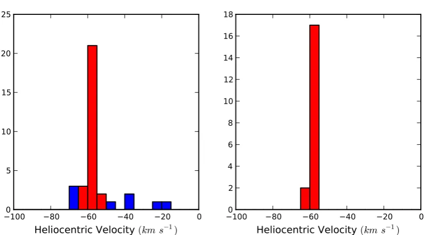
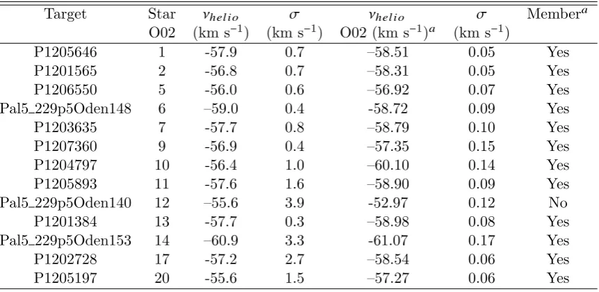
The kinematics of the cluster itself have been studied by Odenkirchen et al. (2002)
(hereafter O02). O02 found the heliocentric velocity of the cluster to be−58.7±0.2 km s−1 with a notably small velocity dispersion of 1.1±0.4 km s−1. Subsequently, Odenkirchen
et al. (2009, O09) provided a kinematic analysis of individual stars in the tails of Pal 5.
Seventeen stars were determined to be members of the tails based on their line-of-sight
velocities. As for the cluster the tails were shown to have a low velocity dispersion: σ <5 km s−1. Such a low dispersion is a defining characteristic of a kinematically cold structure.
The velocities of the stars along the tails also revealed a velocity gradient of ∼1 km s−1 deg−1. These results suggested a revision of the orbit of Pal 5, and O09 further found
that the results are best interpreted if the tails do not align exactly with the orbit of Pal
5, contrary to earlier indications (Odenkirchen et al. 2001). O09 point out the need for
additional kinematic information at larger distances along the tail to further constrain the
simulations of the orbit. Lux et al. (2013) reach similar conclusions.
In this paper we present a self-consistent analysis to identify additional members of Pal
5 and of its tidal tails. In particular we explore the full 20◦ extent of the tails presented
in Grillmair & Dionatos (2006). In the following section we describe the observations and
the analysis techniques employed. In section 3 we discuss our results, first for the cluster
and then for the stars in the tidal tails. Section 4 contains our concluding comments.
2.2
Observations and Data Reduction
2.2.1 Observations and Target Selection
The observations employed for this work were taken with the Anglo-Australian Telescope
(AAT) at Siding Spring Observatory (SSO), using AAOmega, a multi-fibre, dual-beam
spectrograph that utilizes the two degree Field (2dF) fibre-positioning system2. The
sys-tem can allocate up to 392 fibres allowing simultaneous observations of both science targets
and sky regions across a 2◦ diameter field-of-view. The light fed into the spectrograph is
split into the red and blue arms by a dichroic centred at 5700˚A. This work makes use of a
number of observations performed across five years. These include our own observations
§2.2 Observations and Data Reduction 19
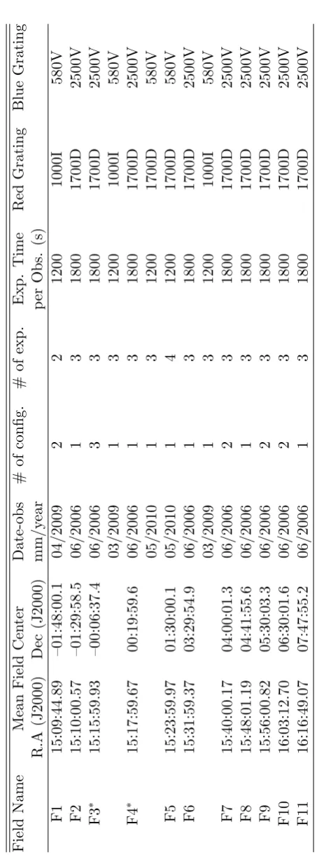
from 2009 and 2010, as well as a set from 2006 (PI: Lewis) obtained from the AAT archive.
In the 2006 June observations, 14 2dF configurations were observed over five nights at nine
distinct field centres spread along the leading and trailing tails. The total integration time
per configuration was 3×30 min. For this run the red arm of AAOmega was configured
with the 1700D grating and the blue arm with the 2500V grating. The red arm spectral
coverage was 8450 – 9000˚A at a resolution ofR ≈10000 while for the blue arm the coverage
was 5280 – 5630˚A at R ≈8000.
The second set of observations took place in 2009 March and April. Completed during
service observing runs, AAOmega was configured with the 1000I grating (spectral range:
8000 – 9500˚A with a coverage of 1100˚A, R =4400) in the red arm and the 580V grating (spectral range: 3700 – 5800˚A full coverage, R = 1300) in the blue arm. In 2009 March single configurations were observed at two field centres while in 2009 April two
configu-rations were observed at a field centre located in the leading tail. The integration times
were 3×20 min for the March observations and 2×20 min for the April set. The final set of
observations used for this work took place in 2010 May, with AAOmega configured with
the 1700D (red arm) and 580V (blue arm) gratings. Single configurations at two field
cen-tres were observed with integration times of 3×20 min and 4×20 min, respectively. Overall
each 2dF configuration typically consisted of approximately 330 targets together with 30
fibres allocated to blank sky regions. Table 2.1 gives an overview of all the observations
used in this work; the total number of stars observed was 4507.
The selection of stars targeted for observation with 2dF varied across the different
runs, and this is illustrated in Fig. 2.1. Both panels display the reddening corrected
colour-magnitude diagram (CMD) for Pal 5 generated from the SDSS DR10 photometry
of Ahn et al. (2014). Only stars within 8.30 of the cluster centre are plotted and the reddening corrections made use of the dust maps available from Schlegel et al. (1998). In
the left panel the approximate region used for target selection for the 2006, 2009 March
and 2010 May observations is delineated, while the right panel shows the approximate
target selection region for the 2009 April run. The reddening corrections to the SDSS
§2.2 Observations and Data Reduction 21
−0.5 0.0 0.5 1.0 1.5
g0−i0
14
15
16
17
18
19
20
21
22
i0
−0.5 0.0 0.5 1.0 1.5
g0−i0
14
15
16
17
18
19
20
21
22
[image:36.595.122.531.103.318.2]i0
Figure 2.1: Both panels show a dereddened colour-magnitude diagram for Pal 5 using
photometry from SDSS DR10 (Ahn et al. 2014). Only stars within 8.30 of the cluster
centre are plotted. In the left panel the blue polygon outlines the approximate target selection region for the observations conducted in 2006, 2009 March and 2010 May. The right panel shows the target selection region for the 2009 April observations.
2.2.2 Reduction and Techniques
Once the data had been extracted from the AAT archive, it was reduced using the 2dF
data reduction pipeline, 2dfdr3. The approach was the standard one using fibre flats
to set the location of the spectra, and arc lamp spectra for the wavelength calibration.
The relative throughput of the fibres, necessary for the sky subtraction, was determined
using theSKYFLUX(MED)approach, which determines the relative throughputs from the
observed intensities of night-sky emission lines. At the end of the process the
wavelength-calibrated sky-subtracted spectra from the individual integrations were median-combined
to remove any cosmic-ray contamination. Typical signal-to-noise ratios (S/N) range from
15 to 70 pixel−1 in the vicinity of the Ca II triplet for the red spectra, and 10 to 40 pixel−1 in the vicinity of the Mg I lines in the blue-arm spectra.
Radial Velocities
The radial velocities of the stars were calculated from the red arm spectra via
cross-correlation using the IRAF4 routine fxcor. The template used for the correlation was
an AAOmega 1700D grating, high signal-to-noise (>100) spectrum of the F6V star HD 160043 taken as part of the program described in Da Costa (2012). The strength of the
Ca II triplet lines in this star match well with those in the program object spectra. The
spectra were correlated over the wavelength interval 8450˚A< λ <8700˚A, a region relatively uncontaminated by night-sky emission line residuals. Heliocentric velocities of the targets
were calculated with theIRAFcommandrvcorrect, and, as discussed in Da Costa (2012),
the uncertainty in the zero point of the radial velocity system is ±0.8 km s−1. Stars that had low correlation peak heights (<0.5) and/or high uncertainties in the correlation
velocity (>5 km s−1) were discarded from the subsequent analysis – generally these were spectra with low signal-to-noise.
A number of stars were observed across multiple fields. We used these multiple
ob-servations to estimate the overall accuracy of the velocities returned by thefxcor routine.
The mean velocity of stars with two or more observations was calculated using the output
errors offxcor as weights. The corresponding estimate of the error for a single observation
was then evaluated using the small number statistics formalism of Keeping (1995), which
utilizes the range of the observations. In particular, the estimated standard deviation for
a single observation is given by:
σ= R×qN (2.1)
where Ris the range in N observations and qN is a multiplicative factor (e.g., q2 = 0.886
and q3 = 0.591). We then compiled these error estimates as a function of the median
signal in the continuum region between the stronger Ca II lines, finding that for stars
with a median continuum level above 1200 ADU the single observation error estimate
was less than 1 km s−1. As the continuum level decreases, the velocity error increases
towards 2 km s−1 at continuum levels ∼700 ADU and then increases rapidly to ∼4 km s−1 at∼200 ADU. These results are consistent with those of Da Costa (2012) who used a similar instrumental setup and analysis technique. We employed this (σv, continuum level) relation to generate the velocity uncertainty estimates for stars with only one observation.
For stars with multiple observations the estimate was reduced by the square-root of the
number of observations.
Photometric Discrimination
Although the primary targets were the stars in the selection boxes shown in Fig. 2.1, the
§2.2 Observations and Data Reduction 23
available 2dF fibres were allocated as possible. However, no unusual stars were discovered,
and since there is no reason to expect any Pal 5 tidal tail stars to lie significantly away from
the principle sequences in the CMD, in the subsequent analysis we focus only on those
stars that lie relatively near to the Pal 5 sequences in the CMD. A routine was created
to remove stars from the data set if their CMD location did not lie within a polygon
encompassing the Pal 5 CMD features, similar to that shown in the left panel of Fig. 2.1.
Giant/Dwarf discrimination
The principle contaminant in the fields containing the Pal 5 cluster and tidal tail stars,
which are giants, are foreground dwarfs of approximately solar metallicity. A means of
distinguishing these stars from the potential cluster and tidal tail members is therefore
needed. We adopt a similar approach to that of Battaglia & Starkenburg (2012), which
employs the gravity sensitivity of the Mg I line at λ8807˚A, a line which is stronger in dwarfs than in giants of similar temperature and metallicity. The discrimination is aided
by the fact that the Pal 5 giants are also metal-poor compared to the vast majority of
field dwarfs. In left panel of Fig. 2.2, we show the relationship between the equivalent
width (EW) of the Mg I λ8807˚A line and the sum of the EWs of the two stronger Ca
II triplet lines at λλ8542 and 8662˚A for the stars in the two fields which contain the
cluster centre. The EW measurements were made using the routinesplot inIRAF. The
uncertainties in the line strengths were estimated from the stars with multiple observations
and are typically 0.15˚A in size. We also identify in the Figure stars that lie within our
adopted radius for Pal 5 (8.30; see§2.3) and within the velocity range encompassing cluster members. As expected, these probable giant stars occupy the lower part of the relationship.
We therefore classify as dwarfs those stars with Mg I λ8807˚A EWs exceeding 0.4˚A, and apply this discriminant to all the observations for which the strength of this feature can
be measured. The adopted value generates a substantial sample of candidate cluster and
tidal tail stars while minimizing the contamination from field dwarfs. It is consistent with
the results of Da Costa et al. (2014) who used a similar approach and a value of 0.35˚A for
the giant/dwarf discrimination. Our value is also broadly consistent with the approach
used in Casey et al. (2013). For those stars in our sample where the S/N of the spectrum
was too low to allow a reliable measurement of the Mg I line strength, an upper limitof
0.14˚Afor the EW value was adopted.
0 1 2 3 4 5 6
EWCa II(◦
A)
0.0 0.2 0.4 0.6 0.8 1.0 1.2
EW
Mg
I
(8807
◦ A)
(
◦ A)
0 1 2 3 4 5 6
EWCa II(◦
A)
0 2 4 6 8 10 12 14
EW
Mg
I
(5180
◦ A)
(
[image:39.595.62.479.100.333.2]◦ A)
Figure 2.2: Left panel: Equivalent width (EW) of the λMg I 8807˚A line as function of the sum of the EWs of the Ca II triplet lines at λλ8542 and 8662˚A for stars in fields F3 and F4, which contain Pal 5. Stars that lie beyond the adopted radius of the cluster (8.30) are plotted as grey points. Blue squares show stars within the adopted cluster radius but outside the velocity range −65 to −50 km s−1, while red triangles show stars within the
adopted radius and within the velocity range. In both cases open symbols are used for stars that are also plotted in the right panel. Right panel: EW of the Mg I triplet features at λλ5172˚A plotted against the summed EW of the Ca II triplet lines, using the same symbols as for the left panel. The dotted line in both panels shows the Mg I EW values used to separate dwarfs from giants.
in the 580V grating in the blue arm was utilized. These features can also provide gravity
discrimination (e.g., Casey et al. 2013). We therefore measured the total EW of the Mg I
triplet lines and the resulting relation between the Mg I line strengths and the Ca II triplet
EW is shown in the right panel of Fig. 2.2. Shown also in this panel are stars within the
cluster radius whose Mg Iλ8807˚A line strengths are available. The form of the relationship is similar to that in the left panel and we adopt a Mg I triplet EW value of 3.5˚A as the
value to discriminate dwarfs from giants. The value is consistent with the dwarf/giant
discrimination discussed in Casey et al. (2012), who used similar 580V observations.
Metallicity of stars
The 2010 on-line version5 of the Milky Way Globular Cluster catalogue (Harris 1996a) lists
the metallicity of Pal 5 as [Fe/H] = –1.41 dex. This value has its origin in the Washington
§2.2 Observations and Data Reduction 25
−3.0 −2.5
−2.0 −1.5
−1.0 −0.5
0.0
V−VHB
1.5 2.0 2.5 3.0 3.5 4.0 4.5 5.0
EW
8542
+
8662
(
◦ A)
NGC288
NGC1904
NGC2298
M30
Figure 2.3: The summed EW of theλλ8542 and 8662˚A lines of the Ca II triplet are plotted againstV−VH Bfor the calibration clusters M30 ([Fe/H] = –2.27), NGC 2298 (–1.92), NGC 1904 (–1.60) and NGC 288 (–1.32). The lines have a gradient α=−0.582 ˚A/mag.
system photometry of Geisler et al. (1997), which yielded [Fe/H] = –1.52± 0.28 (internal
error), and in the high dispersion spectroscopy of 4 Pal 5 red giants analyzed by Smith
et al. (2002) that gave [Fe/H] = –1.28 ± 0.03 (internal error). Since there is no evidence
for any metallicity dispersion in Pal 5, (e.g., Smith et al. 2002) we can use metallicity as
a further means to identity candidate cluster and tidal tail members.
Our metallicity determinations are based on the strength of the Ca II triplet lines in our
spectra, following well-established techniques (e.g., Armandroff & Da Costa 1991). The
calibration of the line strengths is determined from AAOmega 1700D spectra of red giants
in four Galactic globular clusters obtained during other AAOmega observing programs.
The calibration clusters are, in order of increasing metallicity, M30 (NGC 7099), NGC
2298, NGC 1904 and NGC 288. We measured the EWs of the two stronger Ca II lines in
the calibration cluster spectra in the same way as for the Pal 5 program stars. The results
are shown in Fig. 2.3 in which the line strengths are plotted againstV−VH B, whereVH B
is the horizontal branch magnitude in theV-band for each cluster from the 2010 on-line version of the Harris (1996) catalogue. The V magnitudes of the red giant branch stars are generally taken from Stetson’s on-line photometric catalogue6.
The average gradient of the linear least-squares fit to the points for each calibration
cluster is α= −0.58±0.03 ˚A mag−1, a value consistent with other studies. For example,
Yong et al. (2014) find α = −0.60 from a similar set of AAOmega observations. If we