Neural nets their use and abuse for small data sets

Neural Nets - Their Use and Abuse for Small Data Sets

Denny Meyer

I.I.M.S., Massey University Albany Campus, Auckland, N.Z.

[email protected]

Andrew Balemi

Colmar-Brunton Ltd., Takapuna, Auckland, N.Z.

Chris Wearing

Colmar-Brunton Ltd., Takapuna, Auckland, N.Z.

Summary

Neural nets can be used for non-linear classification and regression models. They have a big advantage over conventional statistical tools in that it is not necessary to assume any mathematical form for the functional relationship between the variables. However, they also have a few associated problems chief of which are probably the risk of over-parametrization in the absence of P-values, the lack of appropriate diagnostic tools and the difficulties associated with model interpretation. The first of these problems is particularly important in the case of small data sets. These problems are investigated in the context of real market research data involving non-linear regression and discriminant analysis. In all cases we compare the results of the non-linear neural net models with those of conventional linear statistical methods. Our conclusion is that the theory and software for neural networks has some way to go before the above problems will be solved.

Introduction

With something akin to horror statisticians have been watching the growth in neural net popularity at the forefront of the “data mining” revolution. Mackinnon and Glick(1999) are particularly concerned by the “black box” or “computational algorithm-oriented” nature of neural net rules. It is difficult to trust a model that is not transparent (i.e. cannot be interpreted). Some of the concern is fuelled by the common (mis)conception that data mining (and neural nets) are about automating data analysis and data modelling (Elder and Pregibon, (1996)). Model selection is regarded as a vital part of the statistician’s job and to automate this function may seem threatening to statisticians. However, Chatfield(1995) has warned that statisticians have yet to confront the issues surrounding model selection. In particular he points out that the errors caused by model misspecifation are likely to be far worse than those arising from other sources. He recommends that statisticians should allow for model uncertainty by averaging over several plausible models or by choosing a flexible procedure (such as neural nets) which does not force a particular form of model on the data.

Statisticians are being encouraged to apply and test neural networks (Cheng and Titterington(1994), Warner and Misra(1996)). Faraway and Chatfield(1998) have worked in the context of time series forecasting. Their experience with a relatively small data set suggests that traditional statistical modelling skills should be used in conjunction with neural nets in order to select a good model (with appropriate lags) and that the Bayesian information criterion should be used for comparing different models. In particular Faraway and Chatfield(1998) have stressed problems of over-fitting when predictive error is poor for test data despite good model fits on the training data. However, there is much more neural net experience to be gleaned from the non-statistical literature.

techniques were needed for neural networks before they could be used for medical research. Borggaard(1995) has investigated the use of neural nets for building non-linear regression models for a small data set. He comments on the advantages of using only the major principal component scores instead of numerous raw input variables for regression models. Having only a few variables results in smaller networks, which are quicker to train and easier to optimise in a global sense. Markham and Ragsdale(1995) considered the use of neural networks for classification problems involving small data sets. They found that neural networks do not always outperform classical discriminant analysis as a classification tool and advise that a combination of classical and neural net predictions is more accurate.

In this paper we consider two real examples involving the use of neural networks. The first of these examples involves non-linear regression and the second involves classification. In these examples we confront the problems of over-parameterization, diagnostics and interpretation for small to medium-sized data sets and we compare our results with those obtained using conventional statistical procedures. We discuss methods for minimising the number of input variables and the number of hidden nodes, we consider residual plots as one possible diagnostic tool, and we show how visualisation tools can be used to further prune the number of input variables and for model validation purposes. This paper follows the view of Nelder(1999) that P-values have led to the formation of inferentially uninteresting linear models, suggesting that scientific theory, common sense and visualisation provide better ways to test a model. It is suggested that the realism of the models developed by neural nets, as displayed in “What-If?” Plots gives neural net models an edge. However, the availability of appropriate tools for pruning, testing and interpreting these models is limited and we must agree with Maindaonld’s (1998) warning that “The theory and software have not yet been developed to a point where neural nets are everyday tools for practising statisticians.”

2. Methodology

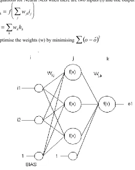
Equations for Neural Nets when there are two inputs (i) and one output (o).

h

=

f

w

i

j

å

æ

è

ç

ç

ö

ø

÷

÷

ˆ

o

=

w

h

k

å

Optimise the weights (w) by minimising

å

(

o

−

o

ˆ

)

Figure 1: What is a neural net?

In Figure 1 the nodes i1 and i2 denote the two input or explanatory variables while o1 indicates the single output or response variables. The second column of nodes (circles) represent the hidden nodes (h1, h2,h3). Associated with each pair of nodes in succeeding layers is a weight (w). These weights are

used to define a linear function of input variables for each node in the next layer. The weights associated with the BIAS nodes are the constant terms.

The linear functions of input variables are transformed using an activation function (f), which often acts as a threshold switch in that it outputs values close to zero or one. Sigmoid and tanh functions are commonly applied in this way, but for the final layer a linear activation function is often used. When a neural net is trained the weights are changed using an iterative procedure which seeks to minimise the difference between the observed and predicted values for the final layer of variables. The initial set of weights is chosen randomly so it is advisable to check that the final solution is a global optimum rather than a local optimum. This can be done by using several sets of initial weights and comparing the final models in each case.

The overfitting problem, which is a particular problem for small data sets, is addressed by using a validation data set. The training data set is used to determine what weight adjustments are required, however, these adjustments are made only if they produce an improvement in predictive accuracy for the validation data set. The software package we used for our non-linear regression and classification examples (Neural Connection, marketed by SPSS) handled this procedure automatically for us. The data were standardised with a mean of zero and a standard deviation of one so as to ensure that all variables contributed equally to the analysis.

Two data sets are used in the analyses that appear below. These data sets were kindly provided by Colmar Brunton Ltd. with the permission of the associated clients but have been suitably disguised. The first data set concerns the market shares, prices, advertising and promotion in a New Zealand cold drink market during a 61 week period. We shall use these data to model the share for three cold drink brands. Such models are useful for predicting the effects of price changes, advertising and promotion decisions on market share. In the second data set demographic and attitudinal data for 2010 people have been used to segment this cold drink market. Such clusters are useful for targetting advertising and for product repositioning exercises. Weekly samples are used to track the performance of brands and adverts for each of these clusters. In both the above analyses conventional linear approaches are compared with non-linear neural net approaches. A combined approach was applied when fitting the neural net models, in that conventional stepwise linear procedures were used to identify the most important input variables.

3.

Our analysis is performed from the perspective of a business that produces three cold drink brands. Two of these brands (True Treat and Northern Delight) compete at the low end of the youth cold drink market, while the third brand (Burgen Broth) is a health drink competing at the top end of what constitutes a different market. The youth and health cold drink markets are distinctly different in that the youth cold drink market is extremely price sensitive while the health cold drink market is not sensitive to price, in fact prices are pretty much fixed. The effect of a change in price is immediate for the youth cold drink market so it is not necessary for us to consider any time lags in this model. The health cold drink market is sensitive to advertising expenditure, especially TV advertising, but the effect of this advertising is not immediate, suggesting that we need to allow for lags in the advertising variable when we predict the share for health cold drinks.

Market Share Model for True Treat and Northern Delight

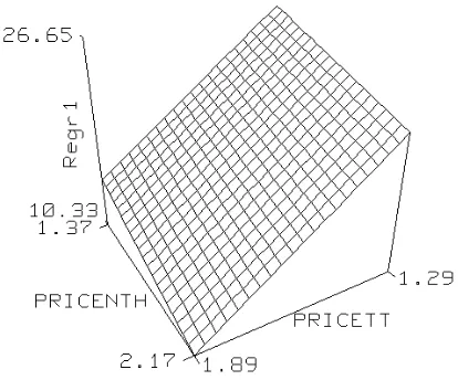
In the case of the youth cold drink market there were 11 variables which were though to affect the relative shares. The share for our business, supplying True Treat (TT) and Northern Delight (NTH), was modelled in terms of these 11 variables using a regression model and a neural net model. As expected the linear regression model indicated an over-parameterised model with the majority of the coefficients (weights) insignificant. In addition it suggested an outlier in a week during which prices for one brand had been cut below cost. Removing the insignificant coefficients and the outlier produced what Nelder(1999) would call “an inferentially uninteresting linear model”,

)

(

67

.

4

)

(

3

.

19

2

.

57

PRICETT

PRICENTH

SHARE

=

−

−

Figure 2: Regression Model: Effect of prices on share

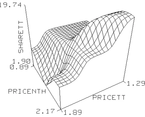
Applying a neural net to these same data in order to predict the market share for True Treat (TT) and Northern Delight (NTH) separately, the Neural Connection package chose to include four hidden nodes. No P-values were obtained in the output, and no information regarding outliers was supplied. The model for TT market share, as illustrated in Figure 3, was anything but uninteresting. The idea of market saturation levels (when falling prices failed to affect market shares) was particularly interesting, as was the apparent pleat in the surface at high TT prices. Such obviously over-parameterised figures are to be expected when data sets are small and the number of neural weights is high. In this case we had 53 weights (44 coefficients for the inputs, 4 coefficients for the hidden layer nodes and 5 constant

Figure 3: Over-parameterized Neural Net Model: Effect of prices on share

Radical pruning of the model was required. After removing the outlier identified previously, the number of hidden nodes was reduced to the minimum required for a non-linear model (i.e. two) and instead of trying to predict the share for both products the output variable was defined as the share for True Treat and Northern Delight combined. In addition to the two predictor price variables (PRICETT and PRICENTH) a variable called PROBLEM was included in the model because it was thought to be particularly important. This variable was an indicator variable defined equal to one only in those weeks in which it was thought that a major problem on the manufacturer’s premises had affected sales. The following equations were obtained for the hidden nodes using a training data set of 54 randomly chosen weeks and a validation data set consisting of the remaining 6 weeks. In these equations x1=PRICETT,

x2=PRICENTH and x3=PROBLEM. The means and standard deviations for these variables are shown as

x

h

=

tanh{0.04

−

0.35

x

−

x

s

æ

è

ç

ç

ö

_ø

÷

÷

+

0.12

x

−

x

s

æ

è

ç

ç

ö

_ø

÷

÷

−

0.30

x

−

x

s

æ

è

ç

ç

ö

_ø

÷

÷

}

h

=

tanh{

−

0.08

+

1.52

x

−

x

s

æ

è

ç

ç

ö

_ø

÷

÷

+

0.43

x

−

x

s

æ

è

ç

ç

ö

_ø

÷

÷

+

0.44

x

−

x

s

æ

è

ç

ç

ö

_ø

÷

÷

}

The coefficients (weights) in these equations suggest that the first hidden node measures the effect of PRICENTH as opposed to PRICETT and PROBLEM, while the second hidden node measures the effect of all three of these variables with most weight given to PRICETT. The final share (y) was predicted using the following equation in which

y

)

17

.

0

51

.

0

12

.

0

(

ˆ

y

s

h

h

y

=

+

+

−

period market share rose when Northern Delight’s price was relatively high in comparison with True Treat.

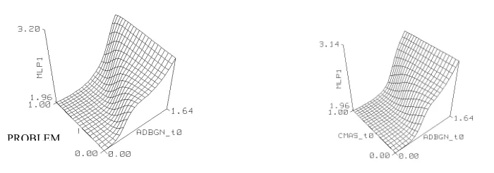
This model can be interpreted using two plots. In Figure 4a the PROBLEM variable is set at zero, indicating no problem and in Figure 4b the PROBLEM variable is set at one indicating a week in which the PROBLEM was affecting sales. The surface without the problem is obviously higher than the surface with the problem, indicating that the problem adversely affected market share. The other interesting feature of these graphs is the range of PRICETT values in which SHARE is very sensitive. Without the problem Share is sensitive to PRICETT for prices of more than about $1.60. This means that there is no point in reducing prices below $1.60 because it will have very little effect on share. However, with the problem effect present the sensitive range reduces to $1.50-$1.70, again indicating the adverse effect of the problem because demand falls faster in response to price increases in the presence of the problem.

NO PROBLEM EVIDENT

2 2. 1 . 2 0 . 2 9 . 1 8 . 1 3 .

1 1.7

0 1

PRICENTH

4 . 1 5 1 6 . 1 5 . 1 0 2 6 .

1 1.5

5 2

7 .

1 _1.8 1.4

E R A H S 9 . 1 1.3

T T E C I R P

Figure 4a: Visualisation:

Effect of prices on share of the youth cold drink market when there is no problem effect

PROBLEM EVIDENT

2 2. 1 . 2 0 . 2 9 . 1 8 . 1 3 .

1 1.7

0 1

PRICENTH

4 . 1 5 1 6 . 1 5 . 1 0 2 6 . 1 5 . 1 5 2 7 .

1 _1.8 1.4

E R A H S 9 . 1 1.3

T T E C I R P

Figure 4b: Visualisation:

The above graphical analysis has served two purposes. Firstly it has validated the model in that it has confirmed that our model is sensible and, secondly, it has allowed us to interpret the model in a more useful manner than was possible using only the coefficients (weights). Increased prices are associated with reduced share, especially in the case of the dominant brand (TT) and the problem clearly had a negative impact on share. As is to be expected the relationships between these variables are definitely non-linear and the regions of price sensitivity are of great financial importance.

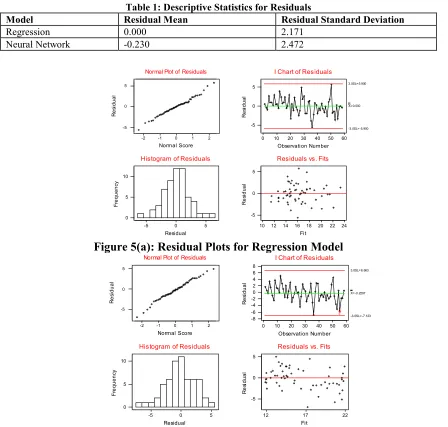
We must now turn back to Figure 2 and ask whether the neural network model is superior to the regression model. Figure 4 seems to suggest that the neural network model is more realistic but what of the behaviour of the residuals? Table 1 indicates that the residuals for the neural net model do not have the appealing characteristic of a zero mean, and the residual standard deviation is larger for the neural net model suggesting an inferior fit. For the sake of consistency the same standard formula for sample standard deviation has been used despite the differing number of coefficients for the two models. However the plots in Figure 5 suggest that the residual behaviour for both the neural net and regression model is reasonably good (i.e. random and approximately normal in distribution). Indeed there seems to be some similarity in these plots.

Table 1: Descriptive Statistics for Residuals

Model Residual Mean Residual Standard Deviation

Regression 0.000 2.171

Neural Network -0.230 2.472

5 0 -5 10 5 0 Residual F req ue nc y

Histogram of Residuals

60 50 40 30 20 10 0 5 0 -5 Observation Number R e si du al

I Chart of Residuals

X=0.000 3.0SL=5.900 -3.0SL=-5.900 24 22 20 18 16 14 12 10 5 0 -5 Fit R e si du al

Residuals vs. Fits

2 1 0 -1 -2 5 0 -5

Normal Plot of Residuals

Normal Score R e si du al

Figure 5(a): Residual Plots for Regression Model

5 0 -5 10 5 0 Residual F re quenc y

Histogram of Residuals

60 50 40 30 20 10 0 8 6 4 2 0 -2 -4 -6 -8 Observation Number R e si dual

I Chart of Residuals

5 X=-0.2297 3.0SL=6.663 -3.0SL=-7.123 22 17 12 5 0 -5 Fit R e si dual

Residuals vs. Fits

2 1 0 -1 -2 5 0 -5

Normal Plot of Residuals

Normal Score

R

e

si

dual

The above analysis has suggested that regression models can provide more accurate predictions than neural net models although the latter models appear more realistic. Residual and predicted value plots have been successfully used for diagnostic checking and interpretation of the neural net models. However, these are rather simplistic tools and with more input variables the predicted value plots would have been awkward.

Market Share Model for Burgen Broth

We now consider the third (health) cold drink, that is Burgen Broth (BGN). As noted previously the health cold drink market is not price sensitive and advertising was expected to have a lagged effect on market share. Market knowledge and conventional stepwise regression were used to select only four of the available input variables for a neural net model. The market share for the following week (y) was

predicted using this week’s share (x1), the effect of Christmas (x2), the problem (x3) and advertising spend

(x4) in the following neural net model

h

=

tanh{

−

3.16

+

1.45

x

−

x

s

æ

è

ç

ç

ö

_ø

÷

÷

+

0.10

x

−

x

s

æ

è

ç

ç

ö

_ø

÷

÷

+

0.17

x

−

x

s

æ

è

ç

ç

ö

_ø

÷

÷

+

0.65

x

−

x

s

æ

è

ç

ç

ö

_ø

÷

÷

}

h

=

tanh{

−

0.68

+

0.83

x

−

x

s

æ

è

ç

ç

ö

_ø

÷

÷

+

1.15

x

_s

−

x

æ

è

ç

ç

ö

_ø

÷

÷

+

1.74

x

_s

−

x

æ

è

ç

ç

ö

_ø

÷

÷

−

2.45

x

_s

−

x

æ

è

ç

ç

ö

_ø

÷

÷

}

)

ˆ

60

.

0

ˆ

83

.

1

50

.

1

(

ˆ

y

s

h

h

y

=

+

+

−

(7.7)

In the first hidden node this week’s share has the biggest impact, but advertising spend is also important. This equation suggests that there are short-term trends in share with share rising in response to advertising expenditure. In the second hidden node a negative impact for advertising spend appears to be associated with a high initial share, Christmas and the problem. This model is illustrated in Figure 6 for a non-Christmas and non-problem period.

Figure 6: Effect of Advertising on Next Week’s Share for Burgen Broth.

it is clear from the righthand graph that advertising is particularly beneficial for market shares of about 2-3%.

No advertising Full advertising

Figure 7: BGN Share in Consecutive Weeks

Finally Figure 8 shows the influence of first the problem and then Christmas on the effect of advertising on market share. It suggests that advertising had less effect on share at the time of the problem and over Christmas.

Influence of the problem only Influence of Christmas only

Figure 8: Effect of Advertising, Problem and Christmas on BGN Market Share.

A regression model fitted using all the above predictors was severely over-fitted and it was found that the following (autoregressive) time series model was all that was significant.

Share(t+1) = 0.81 Share (t) + 0.46

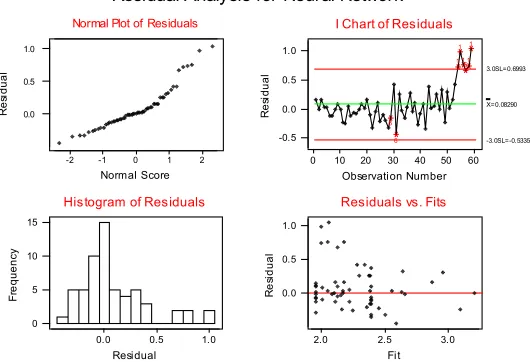
Comparing the residuals for the neural network and the above time series model we obtain the results shown in Table 2.

Table 2: Residual Analysis

Model Residual Mean Residual Standard Deviation

Time Series 0.0044 0.2386

Neural network 0.0829 0.3173

Again it seems that the neural network model produces larger residuals, but in this case the residual plot for the neural net residuals are definitely not random, showing an upward trend over time. This indicates that the neural net model has failed to track the changes in share over time and is therefore inappropriate.

0.5 0.0 -0.5 15 10 5 0 Residual F re quenc y

Histogram of Residuals

60 50 40 30 20 10 0 1 0 -1 Observation Number R e si dual

I Chart of Residuals

7 X=0.004409 3.0SL=0.7670 -3.0SL=-0.7581 3.0 2.5 2.0 0.5 0.0 -0.5 Fit R e si d ual

Residuals vs. Fits

2 1 0 -1 -2 0.5 0.0 -0.5

Normal Plot of Residuals

Normal Score

R

e

si

dual

Residual Analysis for Regression (AR) Model

Figure 9(a): Residual Analysis for Lagged Regression Model

1.0 0.5 0.0 15 10 5 0 Residual F re quenc y

Histogram of Residuals

60 50 40 30 20 10 0 1.0 0.5 0.0 -0.5 Observation Number R e si dual

I Chart of Residuals

6 6

1 1 1₅1

1 X=0.08290 3.0SL=0.6993 -3.0SL=-0.5335 3.0 2.5 2.0 1.0 0.5 0.0 Fit R e si d ual

Residuals vs. Fits

2 1 0 -1 -2 1.0 0.5 0.0

Normal Plot of Residuals

Normal Score

R

e

si

dual

Residual Analysis for Neural Network

Figure 9(b): Residual Analysis for Neural Net Model

In this example the predictive accuracy of a conventional linear model has again surpassed that of a neural net model. In addition the residual plot has shown that the neural net model failed to track the demand behaviour towards the end of the 61-week period. However, the predicted value plots have again suggested that the neural net model is more realistic than a conventional linear model.

of these models but this is largely due to the small number of input variables. Visualisation tools that can easily handle numerous input variables have yet to be developed.

Classification of customers according to their attribute segments

Our third analysis is more data rich in that we have 2010 observations to analyse, with each observation corresponding to a respondent in a survey performed for the youth cold drink market, but, in data mining terms this is still quite a small data set. The data consisted of more than 800 variables including a segment variable with six categories - namely Stable Types, Party Types, Sporty Types, Trendy Types, Independent Types and Discerning Types. The variables tended to be binary (Yes/No), delving into areas such as “Ideal Drink Characteristics”, “Ideal Person Characteristics” and “Ideal Activities and Pastimes”. A parsimonious rule for tracking this segmention was required. This meant that the best variables had to be selected and used to derive a discriminant rule. Two of the variables (cold drink consumption per week and age) were log transformed prior to analysis on account of the skewed righthand tails of these distributions.

Conventional stepwise discriminant analysis (for each segment) was used to select the 43 most important discriminatory variables and the data were analysed using a conventional linear discriminant analysis. The discriminant rule was developed using 90% of the data and was tested on the remaining 10% of the data. The predictive error rate for this test data was 27.6%.

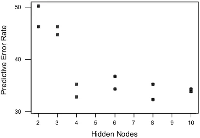
Neural network software has no method for automatically pruning the 800+ input variables so we shall consider only those input variables selected by the stepwise discriminant analysis. The neural network required to classify these data had 43 inputs and 6 outputs, one output for each of the segments. With only 1608 observations in the training data set this meant that we needed at most 6 hidden nodes in order to keep the number of observations per weight above five. However, the default number of nodes suggested by Neural Connection was 24. In the following analysis we varied the number of hidden nodes with two different sets of initial weights in order to determine the optimum number of hidden nodes. A 80%:10%:10% training:validation:test split was applied to the data allowing a proper validation and test of the neural net models. Figure 10 reports the predicted error rate obtained from the test data, suggesting that four hidden nodes is sufficient. This relatively low number is indicative of a fairly linear system which is to be expected on account of the binary nature of most of the variables. The misclassification rate was clearly bigger than the 27.6% achieved with conventional discriminant analysis and this rate was obviously affected by the initial weights, because the predictive error rate varied even when the same number of hidden nodes was used.

10 9 8 7 6 5 4 3 2 50

40

30

Hidden Nodes

P

redi

ct

iv

e E

rro

r R

a

te

Figure 10: Optimising the Number of Hidden Nodes for a Neural Network

Hidden Nodes h1 h2 h3 h4 Important Characteristics

Absent

Rugby Team player

Parties Let Go

Stylish Energetic

Stylish

Important Characteristics

Present Surf/SkateDifferent Discerning

Stylish Boys Older

Clubber

Boys OlderGirls

Segment Hidden Node Weights(w)

Solid Types(O1) 0.73 -0.08 0.26 0.15 -0.12

Social Types (O2) 0.98 -0.14 -0.02 -0.12 0.13

Sporty Types (O3) 0.92 -0.21 -0.11 -0.24 -0.21

Trendy Types (O4) 0.80 0.14 0.18 -0.13 0.11

Independent Types (O5) 0.87 -0.06 -0.15 0.21 0.17

Discerning Types (O6) 0.71 0.35 -0.17 0.13 -0.09

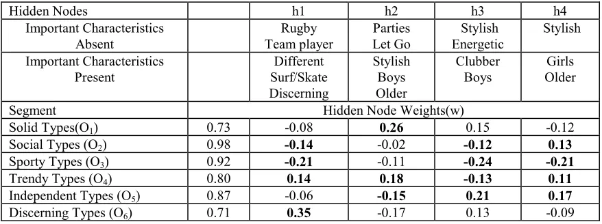
Table 3: Interpretation of Neural Net Discriminant Rules

The Solid segment is obviously identified largely in terms of h2. The Social and Sporty segments

are identified by h1, h3 and h4. The Trendy segment is identified by all four hidden nodes while the

Independent segment is identified by the last 3 hidden nodes. The Discerning segment is identified only by the first hidden node. As expected Solid Types tend to by Older and more Stylish, Social Types are team players, stylish and energetic. So are Sporty types – but more so. Trendy types like to be different, discerning and stylish and Independent Types like parties and letting go, especially in clubs. Discerning Types are just that.

In this example stepwise discriminant analysis has been used to prune the number of input variables before attempting to fit a neural net model. The large number of input variables makes the interpretation of the neural net particular difficult because visualisation is impractical. Instead we are forced to interpret the neural net discriminant rules by considering only the values of the coefficients (weights). It has been found that the neural net model has a lower predictive accuracy than the classical linear discriminant analysis model. No diagnostic check was attempted due to the lack of suitable tools.

4. Conclusion

This paper has found that neural networks can produce some very interesting graphs that allow

statisticians to escape the straight-jacket of linearity. However, it has also shown that neural networks are often too flexible in that they allow unrealistic models to be fitted. In particular, they often allow the use of models with too many coefficients. In the case of conventional (linear) statistics it is possible to prune a data set using stepwise procedures which omit from the model any variable that does not make a

significant contribution. In the case of neural nets there seems to be a lack of such procedures. Neural nets make no attempt to force coefficients to zero when they are insignificant. In addition neural net software packages seem to have no method for minimising the number of hidden nodes automatically.

In this paper it is suggested that a ruthless procedure of pruning be employed whereby any predictor variable that does not make a sensible visual contribution to a model be ignored. In addition it is suggested that the number of hidden nodes be optimised in terms of predictive accuracy. Despite the use of these pruning procedures one of our neural network regression model appears to have badly behaved residuals, suggesting a flawed model. This means that diagnostic checking of residuals is vital for neural nets and needs to be incorporated in all neural net software. There are no specialised tools for doing this, but standard residual plots are reasonably effective.

software. Applying a dimension reduction procedure such as factor or principal component analysis before attempting to fit a neural network, as suggested by Borggaard (1995), will obviously reduce this difficulty, but there is still a need for more powerful visualisation tools.

In our analyses the neural net models failed to match the predictive accuracy of conventional linear regression and linear discriminant analysis, but this may be due to high levels of linearity in the systems studied. It is recommended that many more comparisons of performance between neural nets and conventional statistical regression tools should be performed before an assessment of neural nets is possible in terms of predictive power. Unfortunately such analyses are difficult with current neural network packages, because methods for automatic model pruning and diagnostic checking are not available in most neural network packages. The first priority must therefore be to develop the appropriate theory for pruning and diagnostic checking of neural networks before implementing this theory in neural net software. After this it is necessary for visualisation tools to be developed beyond the current levels, making it easy to understand and explain neural net models.

References

Bishop, C.M.(1995), Neural networks for pattern recognition, Clarendon Press, Oxford.

Chatfield, C.(1995) Model uncertainty, data mining and statistical inference. J.R.Statist. Soc. A, 158(3), 419-466.

Cheng, B. and Titterington, D.M.(1994), Neural networks: A review from a statistical perspective. Statistical Science, 9(1), 2-54.

Duh, M., Walker, A.M., Pagano, M. and Kronlund, K.(1998) Prediction and cross-validation of neural networks versus logistic regression: using hepatic disorders as an example. American Journal of Epidemiology. 147(4), 407-413.

Elder, J.F. and Pregibon, D.(1996) A statistical perspective on knowledge discovery in data bases. In Fayyad, U.M., Piatesky-Shapiro, G., Smyth, P. and Uthurusamy, R.; Advances in Knowledge Discovery and Data Mining. Pp. 83-113, AAAI Press/MIT Press, Cambridge, Massachusetts.

Faraway, J. and Chatfield, C.(1998) Time series forecasting with neural networks: a comparative study using the airline data. Applied Statistics, 47(2), 231-250.

Hair, J.F., Anderson, R.E., Tatham, R.L. and Black W.C. (1998) Multivariate Data Analysis. Prentice-Hall International, Upper Saddle River, New Jersey.

Mackinnon, M.J. and Glick, N. (1999) Data mining and knowledge discovery in databases - an overview. Australian and New Zealand Journal of Statistics, 41(3), 255-276.

Maindonald, J.H.(1998) New approaches to using scientific data statistics, data mining and related technologies in research and research training.

(http://www.anu.edu.au/academia/graduate/papers/gs98_2.html).

McClelland, J.L., Rumelhart, D.E. and the PDP Research Group(1986), Parallel distributed processing: Exploration in the microstructure of cognition, Volume 2: Psychological and Biological Models, Cambridge, MA:MIT Press.

Nelder, J.A.(1999) From statistics to statistical science. The Statistician, 48(2), 257-269.