Near-Lossless Bitonal Image Compression System

Rochester Institute of Technology

RIT Scholar Works

Theses

Thesis/Dissertation Collections

2003

Near-Lossless Bitonal Image Compression System

Jeremy Pyle

Follow this and additional works at:

http://scholarworks.rit.edu/theses

This Thesis is brought to you for free and open access by the Thesis/Dissertation Collections at RIT Scholar Works. It has been accepted for inclusion in Theses by an authorized administrator of RIT Scholar Works. For more information, please [email protected].

Recommended Citation

Near-Lossless Bitonal Image Compression System

By

Jeremy Pyle

A Thesis Submitted

III

Partial Fulfillment of the

Requirements for the Degree of

MASTER OF SCIENCE

III

Computer Engineering

Approved by:

Principal 'Advisor _ _ _ _ _ _

--:--_ _ _ _ _ _ _ _ _ _ _

_

Dr. Andreas Savakis

,

Associate Professor and Department Head

Committee Member

-Dr. Kenneth Hsu

,

Professor

Committee

Member _ _ _ _ _ _ _ _ _ _ _ _ _ _ _ _ _

_

Dr. Marcin Lukowiak, Visiting Assistant Professor

Department of Computer Engineering

College of Engineering

Rochester Institute of Technology

Rochester

,

New York

Release Permission Form

Rochester Institute of Technology

Near-Lossless Bitonal Image Compression System

L Jerem

y

Pyle

,

hereby grant permission t

o

th

e

Wallace Library and the Department of

C

omputer Engin

ee

ring at the R

o

chest

e

r In

s

titute of Technolob'), to reproduce m

y

thesi

s

in

whole or in part

.

Any repr

o

duct

i

on \\ill not be for commercial u

s

c or profit.

J

e

rem

y

C

.

Pyle

,

'

, i

I

~

;'

''''

'

"

)

/I

I /

I ( I : : , <" , ; _" ... I\.. I

i

Abstract

The main purpose ofthis thesis is to

develop

an efficient near-lossless bitonal compression

algorithm and to implementthat algorithm on a hardware platform. The current methods for

compression ofbitonal images includetheJBIG andJBIG2 _algorithms,however both JBIGand JBIG2 havetheirdisadvantages. Both ofthesealgorithms are covered

by

patentsfiled

by

IBM,

making them_costly to implementcommercially.

Also,

_{JBIG only}provides means for lossless compression while JBIG2 provides

lossy

methods _{only for document-type images.} For these reasons a new method for

introducing

loss and _controlling this loss to sustain _{quality is} developed.

The lossless bitonal image compression algorithm used for this thesis is called Block Arithmetic Coder for Image Compression

(BACIC),

which can _efficiently compress bitonal images. In this _thesis, loss is introduced for cases where better compression _{efficiency is}

needed.

However,

introducing

loss in bitonal images is especially

difficult,

because pixels undergo such adrasticchange,either fromwhitetoblackorblacktowhite. Suchpixel

flipping

introduces salt and pepper_noise, which can be very

distracting

when _viewing an image. Two

methods are usedincombinationto controlthevisualdistortion introduced intothe image. The first isto

keep

trackofthe error created

by

the

flipping

of_pixels, and_usingthiserrortodecide

whether

flipping

another pixel will causethevisual distortion toexceed a predefinedthreshold. The second method is region ofinterestconsideration. In this method, lower loss or no loss is introduced into the important parts ofan

image,

and higher loss is introduced into the less important parts. This allows for a good _{quality image} while

increasing

the compression

efficiency.

Also,

the _abilityofBACIC to compress grayscaleimages is studied and

BACICm,

a multiplanarBACIC algorithm, iscreated.

Ahardware implementation oftheBACIC lossless bitonal image compression algorithmisalso designed. The hardware implementation is done using VHDL

targeting

a Xilinx

FPGA,

which

is veryuseful,because ofits flexibility. TheprogrammedFPGAcouldbeincluded inaproduct

Acknowledgements

The author would like to acknowledge the members ofthe thesis committee for their guidance and assistance with theproject: Dr. Andreas

Savakis,

Dr. Ken

Hsu,

andDr. Marcin

Lukowiak,

Table

of

Contents

Chapter 1. Introduction

Page Number: 1

Chapter 2. Image Compression Background 2.1

Entropy

2.2 Image

Encoding

Techniques 2.2.1 Huffman

Coding

2.2.2 Arithmetic

Coding

2.3 Image

Halftoning

2.3.1

Dithering

2.3.2 Error Diffusion 2.4

Lossy

Compression

Chapter 3. Bitonal Image Compression Algorithms 3.1

Group

3

3.1.1

Group

3 1-D 3.1.2

Group

3 2-D 3.2

Group

4

3.3 JBIG 3.4 JBIG2 3.5 BACIC 3 3 4 5 7 10 10 12 14 17 17 17 20 23 24 32 40

Chapter 4. Loss Introduction Algorithms 46

4.1 Background 46

4.2

Greedy

Rate-Distortion

Flipping

49

4.3

Low-Latency Greedy

Flipping Utilizing

Forgetful Error Diffusion 50

4.4 RegionofInterest 53

Chapter 5. HardwareImplementation Overview 5.1 Introduction

5.2 Xess XSV-300

Prototyping

Board 5.3 SRAM Model Module

5.4

Memory

Controller Module 5.5 Divider Module

5.6 Context Generator Module

5.7 BACIC Encoder/Decoder Module 5.7.1 Encoder

5.7.2 Decoder 5.8 System Module 5.9 Testbench Module

55 55 55 56 58 65 66 67 68 72 75 77

Chapter 6. PerformanceComparison

6.1 Lossless Bitonal Image Simulation Results 6.2 Near-Lossless Bitonal Image SimulationResults

6.3 Near-Lossless With ROI Bitonal Image Simulation Results 97

6.4 Grayscale Image Compression Results 103

6.5 Hardwarevs. Software Simulation Performance 106

Chapter 7. Future WorkandDiscussion 109

Glossary

1 1 1

List

of

Figures

Figure 2.1. Huffman

Binary

Tree

Figure 2.2. Arithmetic

Coding

Example

-Step

1 Figure 2.3. Arithmetic

Coding

Example

-Step

2 Figure 2.4. Arithmetic

Coding

Example

-Final Steps

Figure 2.5. Dithered Images

Figure 2.6. Low Resolution Dithered Images

Figure 2.7. Error Diffusion Algorithm

Figure 2.8.

Floyd-Steinberg

Weights

Figure 2.9. Error DiffusedandDithered Images

Figure 2.10. Low Resolution Error Diffusedand Dithered Images

Figure 2.1 1. Modified Peak Signal-to-Noise Ratio

Figure 3.1. Flow Chart for One-Dimensional G3 Compressionstandard

Figure 3.2.

Changing

Element Placement

Figure 3.3. Flow Diagram for Two-Dimensional G3 Algorithm

Figure 3.4. Resolution Reduction Pixel Location

Figure 3.5. Resolution Reductionand Data

Striping

Figure 3.6. Data

Ordering

Figure 3.7. Lowest Resolution Layer Templates

Figure 3.8. Differential Layer Templates

Figure3.9. Deterministic Prediction Pixels

Figure3.10. Sequential Encoder Block Diagram

Figure 3.11.Differential Layer Encoder

Figure 3.12. JBIG Progressive Encoder

Figure3.13. JBIG2 Pattern

Matching

and Substitution Flow Diagram

Figure3.14. JBIG2 Soft Pattern

Matching

Figure 3.15. JBIG2 Template for Refinement

Coding

Figure 3.16. JBIG2 Template for Halftone

Encoding

Figure 3.17.

Gray

Code Example

Figure 3.18. BACIC Templates

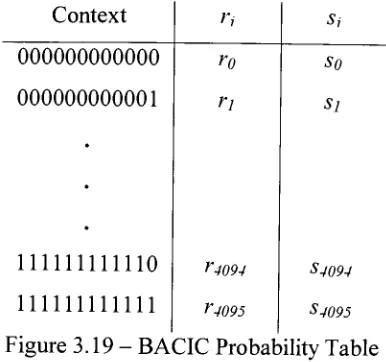
Figure 3.19. BACIC

Probability

Table

Figure 3.20. BACIC Static

Binary Coding

Tree 44

Figure 3.21. BACIC Adaptive

Binary Coding

Tree 45

Figure 4. 1. BACIC Three Line Template Reflection 48

Figure 5.1. XSV-300

Prototyping

Board 55

Figure 5.2. SRAM Model Interface Diagram 57

Figure 5.3.

Memory

Controller Interface Diagram 61

Figure 5.4.

Memory

Controller State Diagram 63

Figure 5.5. Divider Interface Diagram 65

Figure 5.6. Context Generator InterfaceDiagram 66

Figure 5.7. BACIC Encoder/DecoderInterface Diagram 68

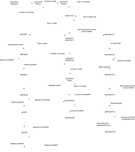
Figure 5.8. BACIC

Encoding

State Diagram 69

Figure 5.9. BACIC Decoder State Diagram 73

Figure 5.10. System Module Architecture 76

Figure 5.11. TestbenchModule Architecture 77

Figure 6. 1. Near-losslessDocument-TypeImages 84

Figure 6.2. High

Quality

Clustered-Dot Lena Image 86

Figure 6.3. High

Quality

Clustered-Dot Peppers Image 86

Figure 6.4. Medium

Quality

Clustered-Dot Lena Image 87

Figure 6.5. Medium

Quality

Clustered-Dot Peppers Image 87

Figure6.6. Low

Quality

Clustered-Dot Lena Image 88

Figure 6.7. Low

Quality

Clustered-Dot Peppers Image 88

Figure 6.8. High

Quality

Dispersed-DotLena Image 89

Figure6.9. High

Quality

Dispersed-DotPeppers Image 89

Figure 6. 10. Medium

Quality

Dispersed-Dot Lena Image 90

Figure 6.11. Medium

Quality

Dispersed-DotPeppers Image 90

Figure 6. 12. Low

Quality

Dispersed-DotLena Image 91

Figure 6.13. Low

Quality

Dispersed-DotPeppers Image 9 1

Figure 6.14. High

Quality

Error Diffused Lena Image 92

Figure 6.15. High

Quality

Error Diffused Peppers Image 93

Figure 6.16. Medium

Quality

Error Diffused LenaImage 94

Figure 6.18. Low

Quality

Error Diffused Lena Image 95

Figure 6.19. Low

Quality

Error Diffused Peppers Image 96

Figure 6.20.

Near-lossless(ROI)

Airplane Image 98

Figure 6.21.

Near-lossless(ROI)

Lena Image 99

Figure 6.22.

Near-lossless(ROF)

Boat Image 100

Figure 6.23.

Near-lossless(ROI)

Monarch Image 102

List

of

Tables

PageNumber:

Table 2.1. Huffman

Coding

Symbol Probabilities 5

Table 2.2. Huffman

Coding

Codewords 6

Table 2.3. Arithmetic

Coding

Example- Symbol Probabilities 7

Table 3.1.

Changing

Elementsfor 2D G3 Algorithm 20

Table 3.2. Vertical Mode Case Description 23

Table 4. 1. Error Diffusion Loss Introduction Parameters 5 1

Table 4.2. Error Diffusion Loss Introduction Parameter Values 53

Table 5.1. Hardware

Memory

Map

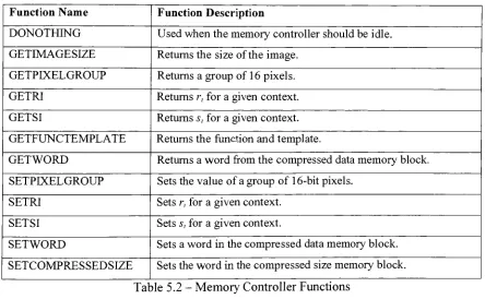
59

Table 5.2.

Memory

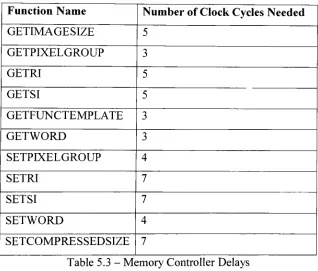
Controller Functions 60

Table 5.3.

Memory

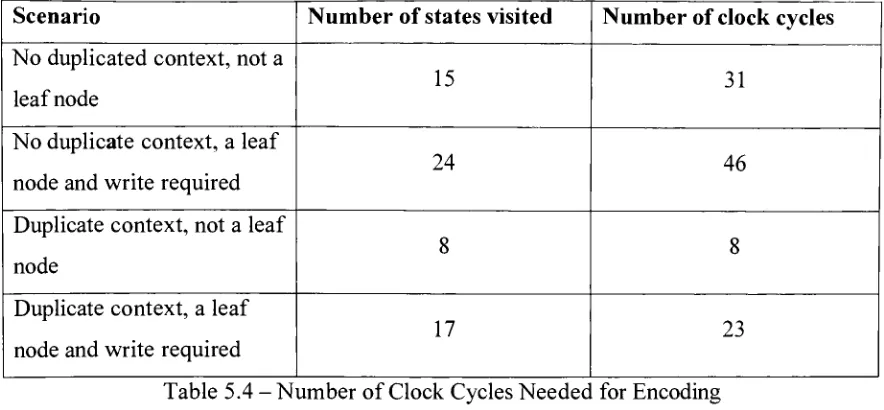
Controller Delays 64

Table 5.4. NumberofClock Cycles Neededfor

Encoding

72 Table 5.5. NumberofClock Cycles Needed for

Decoding

74

Table6. 1. Test Documents 78

Table 6.2. Test Images 78

Table6.3. Lossless Document Compression Results 79

Table 6.4. Lossless Clustered-Dot Compression Results 80

Table 6.5. Lossless Dispersed-Dot Dithered Compression Results 81

Table 6.6. Compression Ratios for Lossless Error Diffused Images 82

Table 6.7. Near-Lossless Compression Results for Document-Type Images 85

Table 6.8. Near-Lossless Compression Results for Clustered-Dot Dithered Images 89

Table 6.9. Near-Lossless Compression Results for Dispersed-Dot DitheredImages 92

Table 6. 1 0.Near-Lossless Compression Results for Error Diffused Images 96

Table6. 1 1.GrayscaleImages 103

Table 6.12. Bitonal Image CompressiononGrayscale Images Compression Results 105

Table6.13. Not

Allowing

Negative Compression 105

Table 6.14. Grayscale Image Compression Algorithm Results 106

Chapter

1.

Introduction

Image compression has been and continues to be a _growing area of interest in the image processing field. As the capabilities ofdigital cameras, scanners and other optical recording

devices improve and the _recording resolution ofthese devices

increase,

the amount of disk storage space neededto storeimages increases.

Therefore,

a needfor imagecompression exists.

There are two main categories of compression algorithms used today: lossless and lossy. A lossless compression algorithm is one in which, after the image has been decompressed each pixel value oftherecovered image is identicalto that ofthe original image [25-27]. Whenthe application requires compression _efficiency that is greater than what can be provided

by

lossless image compression _algorithms,

lossy

image compression algorithms are used

[28-31]

[38]. A

lossy

compression algorithm is one in which the image data ofthe decoded image is not identical to that ofthe source. Near-lossless algorithms

typically

introduce loss in such a waythat the compression _efficiencyincreases _{sufficiently,} but theamount ofloss inthe image isnot noticeable

by

thehuman eye orisnoticeabletoan acceptablelevel.

Near-lossless compression algorithms continue to be a _growing research

interest,

_particularly for bitonal images.

Introducing

loss ina bitonal image is _especially difficult. To introduce loss inabitonal

image,

pixels are flipped meaninga pixel is either changed from a black pixelto a white pixel or vice versa.

However,

ingrayscale or colorimagesthelosscan be introducedtoa much lower

degree,

becausethepixel value canbechanged so that the_{difference is only}afew gray levels or levels of color

depending

on the type ofimage. This pixel

flipping

introduces

salt and paper noise on the bitonal

image,

_greatly

decreasing

the visual _{quality if} distortion

control measures are nottaken.

Compression algorithms can be very complex _{and, therefore,} be costly when _considering

execution _{time, making it beneficial} to implement the algorithm on a hardware platform

[24]

[32-36].

Also,

bitonal images are

typically

used in

faxing

and _printing, so

implementing

the

machine to perform the decompression ratherthan _{requiring the} printer or fax machine to be attachedtoa computertohandlethedecompression.

The compression methods and hardware implementation developed and used in this thesis is

beneficial,

because it provides increased compression for bitonal images as well asthe _ability forthe images to be compressed on a hardware chip. This would become useful in the

faxing

or_{printing industry. If}an enormous documentwere_goingtobeprinted,ratherthan_{waiting for}

theentire lossless imageto be sentto aprinter, some losscouldbe introducedto the document. The document couldthen becompressed and sent to theprinter wherethe _{hardware chip in}the

printer could decompressthe imageandthenprintit out_savingvaluabletime. Thesame is also

trueforafaxmachine.

Following

the introduction in Chapter _1, the rest ofthis thesis isorganized as follows: Chapter

2provides background information intheimagecompressionarea; Chapter 3 discusses lossless bitonal image compression _algorithms; Chapter 4 dealswith the loss introduction algorithms;

Chapter 5 discusses the hardware implantation for this thesis; Chapter 6 presents the results

Chapter 2.

Image Compression

Background

This chapter discusses the fundamentals needed when

dealing

with image compression. It

discusses

terminology

used throughout the image compression

field,

_coding methods used to compress data andimage

halftoning

methods.

2.1

Entropy

When performing image compression, the _{redundancy in} the data is removed. The more

redundancy thatis removed from the imagethe more efficient the compression. For example, for a bitonal

image,

i.e. an image consisting of _only black and white pixels, of size

NxN,

normally N~

bits wouldbe neededto storethe image. However, ifthe image consisted _only of ones,thenitcouldbe stored with_onlyone

bit,

_reducing alldataredundancy.

Entropy

is a well known metric, which defines the amount ofinformation in a bit stream and representsthe lower limit to the amount ofbitsthat can be used with full data recovery. The equationforentropy, H, canbefound below.

H=

-X

P(Cj

)

logP(fl,

)

(Eqn. 2.

1)

whereP(a

),

is the _probability of symbol

a;

. The derivation of this equation can be seen below [5]. A _quantity named self-information is theamount ofinformation stored in an event

E,

andis shownbelow.

1(E)

=log-/-=

-logF(F) (Eqn.

2.2)

r(b)

The above equation states that the amount of self-information stored in

E,

1(E),

is

inversely

proportional to the_probabilityofE. If

P(E)=l,

meaningthat the event is _certain, thenI(E)=0 and no informationis storedin E. This is

because,

if it is knownthatthe event will _occur, then there is no uncertainty, so if it is communicated that the event has _occurred, then no information has_actuallybeentransferred.

base-2 is used forall logarithms unless otherwise specified. Therefore, ifthe_probability of an

event _{occurring is}

V2,

then the information stored inthatevent is I(E)=-log2(1/2)

= ₁

bit. When

one oftwo possible events occurs, each with equal _{probability, then} 1 bit ofinformation is conveyed.

The set of symbols that are transmitted between a sender and receiver is called a source

alphabet, for example A =

{ai,

aj,...,aj}. The _probability that the information source will produce symbol _a, is defined as P(a,). Because the source alphabet is

finite,

the

following

equationholdstrue.

I^)

= l _(Eqn.

2.3)

Avector z isusedtorepresentthe set of all source symbolprobabilities,suchthat

z=_{{P(al),P(a2),...,(P(a}

t)}. The information source can be described completely using the finite ensemble (A,z). Ifk source symbols constitute the symbol _{alphabet, then according} to

the law of large numbers, for a _{sufficiently large} value of

k,

symbol _a} will, on average, be

output

kP(Oj

)

times.

Therefore,

the informationobtainedfrom_observingkoutputs is

L-g

=

-kP(a,

)

\og(P(ax

))

-kP(o2

)

\og(P(a2

))-...

kP(a}

)

log(F(^

))

or

-k^P(aj)log(P(aj) (Eqn. 2.4)

Therefore,

theamountofinformation ineach source_{output, entropy,} denoted as

H(z)

is

H(z)

=

-j^P(aj)log(P(aJ)) (Eqn.

2.5)

7=1

For _example, ifan alphabet consists ofthree symbols _ai, a2 and _a^, with probabilities

0.2,

0.3

and0.5 respectively,then the_entropycanbe found_usingEqn.2.5 as shownbelow.

H(z)

=

-

P(a}

)

\og(P(a}

))

=-(0.2 *

log(0.2)

+0.3*

log(0.3)

+0.5*

log(0.5))

=_AMlbits ;=i

2.2 Image

Encoding

Techniques

Therearethreebasic steps for image compression: mapping,quantization and encoding. In the

inthe_encoding step. Thequantization_step isused for

lossy

compression, where similar pixels canbemappedtothesame symbol. The mappingand quantization_{step decrease}the size ofthe data

by

_reducing the interpixel redundancies. For example, for an 8-bit

image,

if the image consists_entirelyofzeros,then _onlyone symbolisneededtorepresenttheimage.

Several different types of encoders exist to compress image

data,

such as run-length _coding

[17],

Huffman coding

[7],

arithmetic _coding

[17]

and transform _coding [17]. Some ofthese

techniques arediscussed inthe

following

sections.

2.2.1 Huffman

Coding

In

1952,

D.A. Huffmandevelopeda_{coding technique,}which was laternamedHuffman coding.

Huffman coding produces the shortest possible average code length given the source symbol

set and the _{corresponding probabilities, only} ifthe probabilities are exact powers of2. The Huffmanalgorithm canbe broken up into 3 steps:

1. Orderthesymbols accordingtotheirprobabilities.

2. Combinethe twosmallestprobabilitiesintooneto forma parent node

by

_addingthe

twoprobabilitiestogether.

3. _{Repeat step 2}untilthere _{is only}one root nodewith a value of1.0

Each of the nodes are then given a value

by

traversing

the

binary

tree and at each split

appending a T or a

'0"

to the codeword

depending

on which path wastaken. The algorithm

can be best described

by

example. The example shows the codeword construction process of Huffman coding forthesymbols and probabilities showninthe tablebelow.

Symbol

Probability

a 0.05

b 0.05

c 0.2

d 0.25

e 0.45

Table2. 1 - Huffman

The figure below shows the

binary

tree created when

doing

the Huffman codeword construction _usingtheprobabilities shownin Table 2.1.

e 045

c 0 20

b 005

a 005

0 55

jl JK0 0

0 30

1_O10 0

Figure 2.1

-Huffman

Binary

Tree

To create this tree first the symbols were listed in order of

decreasing

probabilities as can be seen _alongthe left side. Next the two smallest probabilities, 0.05 and 0.05 were combined

by

adding them together and

forming

the 0.10 node. The probabilities were then reordered

by

decreasing

probabilitiesandthe nexttwo smallestprobabilities, 0.10 and 0.20, were combined

to formthe 0.30 node. The process repeats until the 1.0 root node was formed. Then at each

combinationaT was assignedto the

top

child node and a0to the bottomchild node as canbe seen in Figure 2.1. The codewords for each symbol arethen found

by

traversing

the tree from

the root node to the _{corresponding} child node and _appending either the '0' or '1"

digit

depending

on which path wastaken. Thetablebelowshows each symbol and its corresponding codeword.

Symbol Codeword

a 1100

b 1101

c 111

d 10

As can be seen in Tables 2.1-2.2 the symbols with the highest probabilities were given the

smallest codewords and the symbols with the lowest probabilities were given the larger symbols,which provides efficient compression.

Huffman encoding is a _very useful compression method when _compressing data in which the

probabilities are all integer powers oftwo. However one disadvantage is the decrease in

compression _efficiency as the difference between the probabilities and the integer powers of

twoincreases.

2.2.2 Arithmetic

Coding

An arithmetic coderis another means of_{reducing the redundancy}in data. An arithmetic coder works

by

_encoding a _group of symbols as a real number in the range of 0 to 1. Several

arithmetic coderimplementations exist such as LZAP

[8],

theLee and Parkalgorithm

[9],

the

Z-coder

[10],

the IBM

QM-coder[ll],

the IBM

Qx-coder[12]

and the Block Arithmetic Coder for Image Compression

[1],

which isused forthisthesis.

There aretwobasicpieces ofinformationthat are neededforarithmetic coding: the _probability of a symbol and its encoding intervalrange.

Any

number of symbols canbe encoded_usingone real number as

long

asthe precision ofthereal numbers is good enough. The example below illustrates howarithmetic _codingworks.

For this example, consider a system with a four-symbol alphabet as shown in the table below

withtheirprobabilities.

Symbol

Probability

a 0.1

b 0.2

c 0.3

d 0.4

Table2.3- Arithmetic

Coding

Example- Symbol

Thenumber of symbols that are _goingto beencoded ineach codeword needstopredetermined

and known

by

both the encoder and decoder. For this example, four symbols are encoded in each codeword. _{The encoding}ofthemessage

"accd"

canbe seenbelow.

Firsteach symbol isgiven a range_accordingto itsprobability. Therange starts from 0to 1, so

symbol *a is given the range 0 to

0.1,

symbol 'b"

is given the range 0.1 to 0.3. symbol

'c'

is

given the range 0.3 to 0.6 and symbol

"d'

isgiven the range 0.6 to

1.0,

as illustrated in Figure 1 9

't

Figure2.2- Arithmetic

Coding

Example

-Step

1

Becausethefirstsymbol inthemessage is

'a',

the interval forthesecond _{step becomes 0}to 0.1. The range isthen _{broken up}again foreach symbol _{using its}probability. Therangefor symbol 'a'

is now 0 to

0.01,

the range for symbol 'b'

is now0.01 to

0.03,

the range for symbol

"c"

is

now 0.04to0.06andthe rangeforsymbol

'd"

isnow0.06to

1.0,

as shownin Figure 2.3.

The next symbol in the message is

'c\

so the interval now becomes 0.03 to 0.06. The same

process is donetwomoretimestoencodethethird andfourthsymbols as can be seenin Figure 2.4. Afterthe _encoding ofthe third symbol

'c'

therange becomes 0.039 to 0.048 andthe range is again broken up into subdivisions. The last symbol in the message is *d', so the message "accd"

Figure 2.3 - Arithmetic

Coding

Example

-Step

2

0 fl 0 00 0 039

a

I

a a

01 _

T 0.01_

J

0 033_ 00399_

-)

03 _

\

\

0 03_ 0 039_ 0 041 7_

06 \

\

\

\

006_

\ \

3 048.

~\

00444_

\

\

\

\

i

1 0 \01 \006 ", 0048

Figure2.4- Arithmetic

Coding

Example

-Final Steps

There are problems inherent in arithmetic _coding which are important to examine before

attempting to implement an arithmetic coder. Since no machine can have infinite _precision, underflow and overflow can be an issue. If insufficient precision is used _considering the

receivesthe entire codeword.

Also,

arithmetic _{coding is}an error sensitive compression scheme,

meaninga singlebiterror cancorrupttheentire message.

There are twobasic types of arithmetic coding: static and adaptive. Instatic arithmetic _coding

the probabilities of each ofthe symbols do not change. With adaptive arithmetic coding, the

symbol probabilities are estimated

during

each _step of the _encoding process based on the

changing symbol frequencies that have been seen in the _previously encoded messages.

Because in the real world the exact probabilities are impossible _{to produce,} it cannot be

expected that an arithmetic coder will achieve maximum _efficiency when _compressing a

message. The bestan arithmetic coder cando istoestimatetheprobabilities onthefly.

2.3 Image

Halftoning

This thesis _{deals primarily}with the compression ofbitonal images. Several algorithms exist

for obtaining abitonal image from a grayscaleimage. The main goal of

halftoning

animage is

to preserve the overall grayscale look ofthe image while _changing each pixel from an 8-bit

value(couldalsobe 4-bitorhigherthan

8-bit)

intoa 1-bitbitonalvalue.

2.3.1 Ordered

Dithering

There are several methods for _converting an 8-bit grayscale image into a 1-bit bitonal image.

Ordered

dithering

is one ofthe simplest methods for

doing

this and involves using a dither

mask [5]. This rectangular mask can be _{any size,} but is usually square. The mask consists of

threshold values between 0 and

255,

for an 8-bit image. The mask is then moved over the

entire image and each pixel is then compared with its correspondingvalue in the dither mask

usingtheequation below.

0

if

_it, ,>m

\1 _{// u,} j

<

m,j

where _{Ujj is} the original pixel atlocation

(ij)

with respectto thedithermask, _{m,j is}thevalue in

the dither mask at position

(ij)

and _uid

'

is the new value ofthe pixel. The reason for the

white pixelhasa value of255 (for

8-bit),

while ina bitonal imageablackpixelhas a value of1

and a white pixelhasa value of0. The dithermask isthenmoved aroundthe entireimageuntil

all pixelshavebeen halftoned.

Another

thing

toconsider when_performingan ordereddither iswhattypeofdithermasktouse.

There are two basic types of dither masks: dispersed-dot and clustered-dot. A dispersed-dot

mask would leavethe blackpixels spread out and not bunched_together, while a clustered-dot

mask would

keep

the black pixels grouped together and the white pixels clustered together.

Dispersed-dot ordered dithers are designedto yield

halftones,

which _conveythe impression of

gray. Clustered-dot ordered dithersare designedto yieldhalftoneswithfew isolatedpixels and

are

typically

used with _printing

devices,

which cannot _properly

display

isolated pixels in an

image. Figure 2.5 shows halftoned images usingthe two differenttypes ofdithermasks, both

masks are4x4pixels.

(a)

Clustered-dot Dithered Image

(b)

Dispersed-dot Dithered Image

Figure2.5- DitheredImages

As canbeen inthe above figure athigh resolutionit is sometimes difficultto tellthedifference

between clustered-dot and dispersed-dot although differences can be seen. The figure below

shows the three figures above except zoomed in on a specific area ofthe image to showthe

"^vv/jyjxw.w.

(a)Clustered-dot Dithered Image _{(b)Dispersed-dot Dithered Image}

Figure 2.6

-Low ResoutionDithered Images

As can be seen when

halftoning

a low-resolution picture, such as the ones shown above in

Figure

2.6,

the visual _{quality decreases} significantly. Even at thisresolution the dispersed-dot

dither still maintains a small illusion ofgrayscale, buttheclustered-dot image haspoor quality.

As expected onthe clustered-dotimagetheblackpixels are clusteredtogether.

2.3.2 Error Diffusion

Anothermethod of

halftoning

is errordiffusion [16]. As the name

implies,

in this methodthe

error created

by

the

thresholding

is diffused to increase the _quality of the halftone. The

diagram below illustratesthe errordiffusion algorithm.

Input

+ _A

Threshold ?Output

Error Filter

Figure2.7-_{ErrorDiffusionAlgorithm}

The algorithm works

by

traversing

the image pixel

by

pixel, in raster scan _order, and

thresholding

each_{pixel, usually}witha value of128 (for 8-bit images). Theerrorforthatpixel

from

0,

depending

onthe color ofthe _{corresponding bitonal}pixel. This error is then diffused

usingthe

Floyd-Steinberg

weights

[16],

shown inthe figure below.

X 7/16

3/16 5/16 1/16

Figure 2.8-

Floyd-Steinberg

Weights

The 'x'

in the above figure is the current pixel. The error created

by halftoning

the current

pixel is then diffused to the _neighboring pixels

by

_multiplying the error

by

the value shown in

Figure 2.8 andthen _addingthat value to the grayscale value forthatpixel. As can be seen in

the above figure the

Floyd-Steinberg

weights _only affect pixels that have not yet been

processed. Thefigure below shows animagethathas been halftoned_usingerrordiffusion.

(a)

Error Diffused Image

W

.U ii

'

. .L .X

X-::'!''. '!j"j!.'. IP*'

\i_*.

mm t- ~

agar;,i5__!* , f^g^I- i

llj:"f.nt'pL-/SS*

(b)

Dithered Image

Figure2.9- Error Diffused

andDithered Images

As can be seen in the above

figure,

the overall grayscale look ofthe error diffused image is

impressive. The error diffused image also looks betterthan the dispersed-dot dithered

image,

because it doesn't have the grid lines thatshow _{up in}thedithered image. Below shows a

i.:;*.*..'

Fi'tf

i

(a)

Error Diffused Image

itiix ::::sftftaofsrtnocv. v.

:-:::-:>:':: :: :: :-:M':-:':-:':-:::-:::-:::-::i:::::

(b)

Dithered Image

Figure 2.10

-Low Resolution Error DiffusedandDithered Images

As can be seen in the low resolution images in Figure

2.10,

the error diffused image still has

much better quality than the dithered image. Obvious differences now appear between the

error diffused and the original

image,

but unlike the dispersed-dot dithered image theobject in

theimage is_easilyrecognizable.

2.4

Lossy

Compression

Digital image compression algorithms can be classified intotwo categories: lossless and lossy.

A lossless compression algorithm is one in which afterthe image has been decompressed each

pixel value of the recovered image is identical to that of the original image. A

lossy

compression algorithm is one in whichthe image data ofthe decodedimage is not identical to

thatofthesource.

The goal of a

lossy

compression algorithm is to improve on the compression ratio while

keeping

the visual distortion to an acceptable level. Compression ratio is defined _{using the}

equation shownbelow.

CompressionRatio=

Originalimagesize

Compressed imagesize

(Eqn. 2.

7)

The level of acceptable visual distortiondepends onthe application. There are several metrics

thatcanbeusedtomeasurethedistortion,such as root mean-squared-error

(RMSE)

and

signal-to-noise ratio (SNR). In image coding the peak signal-to-noise ratio

(PSNR)

is more

The RMSEis defined_usingtheequation shownbelow.

1 i N-l M-\

RMSE=

Y

j(x

-v )2

\N Mtt

j^'-J -'"'J (Eqn.

2.8)

where _{xjj is} the pixel in the original image at location _{(ij), v,,, is} the pixel in the compressed

imageat location

(ij),

Nistheheight oftheimageandMisthewidth oftheimage.

Thepeak signal-to-noise ratio is defined inthe equationbelow.

255 PSNR =20

log

₁₀

RMSE

(Eqn.

2.9)

Because the focus ofthis thesis is bitonal image compression, the PSNR metric alone is not

veryuseful. Thereason isthateach pixel can consist_onlyof a0or

1,

sothe_onlyerrorthatcan

exist is 1. Another choiceisto use 0 and 255 asthe pixel _values,then the error would be 255.

However,

this isalargeerror amount and couldbe misleading inthat _{for only}one pixel errorin

a region, the value ofthe error could be rather large. To better approximate the perceived

grayscale error a metric called the modified peak signal-to-noise ratio

(MPSNR)

is used [21].

Forthis metric, the inverse

halftoning

ofthe bitonal image is done

first,

andthen the PSNR is

taken. In order to do the inverse

halftoning

a Gaussian Low Pass Filter isconvolved with the

originalbitonal

image,

as canbe seenintheequationbelow.

G= 100

1 2 4 2

2 4 8 4 2

4 8 16 8 4

2 4 8 4 2

1 2 4 2 1

(Eqn.

2.10)

H,

=H*G

Using

Equations

2.10-2.11,

the inverse

halftone,

//_,,.,

of H is found. The MPSNR is then

found _{using Equation}

2.9,

_using the original grayscale image to do the comparison. The unit

for Equation 2.9 is decibels (dB).

The images in Figure 2.1 1 showthevalues oftheMPSNRfor different levelsof noise addedto

the Lena image. Image

2.11(a)

is the lossless grayscale image. Image

2.11(b)

is the lossless

error diffused Lena image. Images

2.11(c)

through

2.11(f)

are the error-diffused image with

increasing

amounts of salt and pepper noiseadded. Ascanbe seeninthe

figure,

asthe amount

of noise

increases,

theMPSNR

decreases,

as expected.

(b)MPSNR=25.7747dB (c)MPSNR=25.3156dB

(d)MPSNR=24.8631dB (e)MPSNR=24.0405dB (f)MPSNR=22.7038dB

Chapter

3.

Image Compression

Algorithms

There are several algorithms and standards that exist

today

forthe compression ofimages. As

was stated _above, the goal of lossless compression algorithms is to reach a compression

efficiency equal to the entropy. This chapter discusses several bitonal image compression

standards and _algorithms, one of which is used for this thesis. The other compression

algorithms are

discussed,

because

they

show other means for bitonal image compression. The

bitonal compression algorithm used for this thesis improves upon the deficiencies of those

algorithms.

3.1 CCITT

Group

3 Compression Standard

The Consultative Committee onTelephone andTelegraph

(CCITT)

developedthe

Group

3 Fax Algorithm

(G3)

in 1980 [18]. The G3 compression standard was developedfor digital facsimile

transmission on the public switched telephone network. The main goal of this bitonal

compression algorithm was to be able to compress a document scanned at 100 dots per inch

(dpi)

and sampled at 1728 samples per lineto betransferred at4800 bitsper second

(bps)

inan

averagetime of about one minute. This meansthat inorder to transmita standard 8.5x11 inch

pageinthe_{time needed,} a compression ratio of about6.6 isneeded.

The G3 algorithm works

by

_counting the size ofblocks of either all ones or all zeros and

encoding this count. This method takes advantage of the

tendency

oftextual documents to

include a lot of white space, because between each letter and between lines of a textual

documentis white space. There aretwo alternate_coding schemes inthe G3 algorithm: CCITT

Group

3 one-dimensional and CCITT

Group

3 two-dimensional.

3.1.1 CCITT

Group

3 One-Dimensional Compression standard

The CCITT

Group

3 one-dimensional _coding scheme encodes an image as a series ofvariable

length codewords, so that each codeword represents ahorizontal blockof either all white or all

black pixels. The codewords used are the Modified Huffman

(MH)

code. The Modified

Huffman code has two types ofcodewords:

Terminating

codewords and

Make-up

codewords.

of0 to 63.

Make-up

codewords are used with

terminating

codewords to encode blocks larger

than63 pixels. These make-up codewords canhandlepixel blocksofsize 64to 1728. Forrun

lengths larger than 1728 an optional set of_make-up codewords canbe used which can encode

run lengths _upto 2560 _pixels, which would beused when

transmitting

documents at a higher

resolution.

An End-Of-Line

(EOL)

codeword exists to _signify eitherthe start of an image or the end of a

line. Attheend of animage a special codewordis used calledReturn To Control

(RTC)

which

consists of 6 EOL codewords. The flow diagram shown in Figure 3.1 illustrates the

one-dimensional

Group

3 compression standard.

As can be seen in the flow

diagram,

the algorithm starts

by inserting

an EOL _character, as a

rule withthis _algorithm,anEOL must existbefore the _encodingofthefirst line. Then thefirst

runis counted and encoded accordingly. Therearethree tables thatare usedforthis algorithm:

Terminating

codes table (T

Table),

Make-up

codes table (M

Table)

and Additional

Make-up

codes table (AM Table). The T Table consists of 128 codewords for all different run-lengths,

white or

black,

from 0 to 63 pixels.

Therefore,

if a run exists of length 0 to 63 it can be

encoded withjustone codewordfromthis table. The M Tableconsists of55 codewords. Ithas

a codeword for multiples of64 from 64 to 1728 and an extra one

defining

EOL.

So,

ifa run

length is in the range of64 to

1728,

it is encoded as a codeword from the M Table and a

codeword from the T Table. Finally, the AM Table is usedto handle runs oflength 1792 to

2560. It is just an extension ofthe M

Table,

so ifa run were oflength 1792 to

2560,

itwould

be encoded_usinga codewordfromtheAM Table and acodewordfromtheT Table.

For_example, ifa run of40 blackpixels exists, then theT Tableisusedtofindthecodewordfor

a run of40 black pixels (000001101100). So

"000001101100"

is the _encoding of40 black

pixels. Ifa run of100white pixels exists first theMtable wouldbe _{used, using}thecodeword

for 64 white pixels

(11011),

since 64 is the biggest multiple of64 less than or equal to 100.

Then the T Table is used to findthe codeword for 36 white pixels

(00010101),

because 100

-64 = _{36. So}

Looking

atthese

tables,

which can be found in

[18],

it canbe seenthat the encoding of white

pixels has smaller codewords than for black pixels. This is because the G3 compression

standard was made _{primarily for} facsimile transmission. Facsimile transmission consists

mostly oftextual

documents,

whichhave a lotof white space inthem. This allowsfortextual

documentstocompress efficiently.

Begin

T

Countarun

Run-length <1792?

Run-length <64?

Look up T Table

Endof Line?

T

EOL

Endof Image?

Look up M Table

Look up AM Table

Reducerun-length

Reducerun-length

T

RTC

Figure 3.1 - Flow Chart forOne-DimensionalG3 Compression

3.1.2 CCITT

Group

3

Two-Dimensional

_{CompressionStandard}

The problem with the one-dimensional

Group

3 algorithm is that _{it only} takes advantage of

runs in the

horizontal

direction. In a textual document runs exists in both the horizontal and

vertical

directions.

Therefore,

_inordertoget even greater compression_efficiencythealgorithm

must take advantage ofthe vertical runs as well. The two-dimensional

Group

3 algorithm

explores correlation of pixelsintheverticaldirectionas well asthehorizontal direction [18].

Both the one-dimensional and two-dimensional

Group

3 algorithms use a line-by-line _coding

method. In _{the two-dimensional algorithm, a reference element is used which determines the}

mode in which the current _group of pixels will be coded. The reference element can either

exist on the _{line currently}

being

_coded, called the _coding

line,

or the previous

line,

called the

reference line. After the entire _{coding line has been processed,} it becomes the reference line

and the next _{line down becomes} the _{coding line.}

However,

_{one problem with}

coding a line

while

taking

into account the previous line is that ifthere is a transmission error on one

line,

then allthelinesafterthatcan bewrong. To avoidthisproblemthetwo-dimensional algorithm

periodically sends a _{line using}theone-dimensional G3 algorithm. Thisperiod is knownas the

Kfactor. Kcan _{be any}positive integer. Inother wordsfor every K

lines,

1 ofthemisencoded

usingthe one-dimensional _algorithm, and K-l ofthemare encoded _using the two-dimensional

algorithm.

There are five pixels usedto determine which mode and howeach _group of pixels is encoded

which arelisted in Table 3.1.

Changing

Element

Definition

a0 Thereference element onthe_{coding line.}

ai Thenext element onthe_{coding line}to theright ofa0andtheopposite color of ao.

a2 Thenext element onthe_{coding line}totheright ofai andtheopposite color of aj.

bi

Thenext element onthereferencelineto therightof_a0andtheopposite colorofa0.

b2

Thenext element onthereferencelineto theright ofh. andtheopposite color ofb..

Table3.1

The element _ao is set from the previous iteration of _{the algorithm,} and at the

beginning

of

encoding it is set to an

imaginary

white pixel beforethefirstpixel ofthe image. The example

in Figure 3.2 showstheplacement ofthe_{4 changing}elements with respecttoa0.

Ref. Line

Coding

Line

a a

0 /

Figure 3.2

-Changing

Element Placement

[17]

a

Therearethree_coding modes usedinthetwo-dimensional G3 algorithmthat aredetermined

by

the position ofthe _changing elements shown in Figure 3.2: Pass

Mode,

Vertical Mode and

Horizontal Mode. Pass Mode is used when the position of

b2

lies to the left of aj. Vertical

mode is used when the relative distance between _ai and

bi,

_meaning the distance between _ai

and

bi

if

they

were onthe same

line,

is lessthan or equal to3. Horizontal mode isused when

neitheroftheothertwo modes applies.

Each ofthe modes described above gets a set ofdistinct codewords. For Pass Mode there is

only one codeword that is ever used 0001. The coding ofthe location ofthe other _changing

elements is not needed. For Horizontal Mode the codeword is

001+M(a0ai)+M(aia2),

where

a;aj is the length and color ofthe run between a, and aj. For example in Figure

3.2,

_a0ai is a

white run of3.

M(a;a,)

is the codewordused inthe one-dimensional G3 algorithm foundinthe

M Table. There are 7 cases forthevertical mode,

depending

on where ai iswith respect to

bi,

each withitsowncodeword. Table 3.2 describesthesedifferent cases.

Put_a0justbefore 1"_pixel

Detectb.

b.tothe leftof a,7

Begin

No Yes

1a LineofK lines?

Verticalmode

coding

Putanon_a,

iPassmodecoding

T

No

Endof Line?

T

Put_a0justunder

b,2 Yes

T

EOL

EOL+ 1

One-dimensional coding

Detecta.

Horizontalmode

coding

Puta. ona,

Endof Image9

Yes

RTC End

Case Description Codeword

V(0)

ai isjustunder

bi

1

VR(1)

ai isonepixelto theright of

bi

Oil

Vr(2)

ai istwopixelsto therightof

bi

000011

Vr(3)

aiisthreepixelsto theright of

bi

0000011

Vl(1)

ai isone pixelto theleftof_bi 010

VL(2)

aiistwopixelsto theleftofbi 000010

VL(3)

aj isthreepixelsto theleftof_bi 0000010

Table 3.2

-Vertical Mode Case Description

As shown in Figure

3.3,

thealgorithm starts

by

_checkingto see ifthe current lineisthefirst of

K

lines,

andifit

is,

it doesone-dimensional coding. If it isnot,thenaois placedjust beforethe

firstpixel and at, bi and

b2

are found. Afterthosethree _changingelements are

found,

themode

of_coding, is foundandthepixel_{group is} encoded accordingly. ThenaO isrepositioned andthe

whole process starts over again with the detection of_ai,

bi

and b2. After the entire line has

been coded,thealgorithm checks toseeiftheimage is

done,

ifnot, it starts over again withthe

checkingtoseeifthisisthefirstofK lines.

3.2 CCITT

Group

4Compression Standard

In

1984,

the CCITT

Group

4

(G4)

compression standard was developed as a facsimile coding

scheme forthe compression ofblack and white images [19]. The standard is designed strictly

for error-free digital facsimile transmission, and it assumes that all error correction is already

handledon a lower levelofthecommunicationprocess.

The

Group

4 standard works _very similar to the two-dimensional G3 standard. The main

difference between the two standards is that the two-dimensional G3 algorithm _periodically

encodes entire lines _using the one-dimensional G3 method, but the G4 algorithm encodes all

lines _using the two-dimensional G3 algorithm. When the G4 algorithm

begins,

it inserts an

imaginary

whitelineabovethe first lineoftheimagetobethe firstreference line.

The main advantage ofthis method over the two-dimensional G3 algorithm is the improved

algorithm does one-dimensional _{encoding every K}

lines,

and one-dimensional _coding lowers

thecompression _efficiency, becauseit does nottake into account runs inthe vertical direction.

However,

robustness is a major problem withthe G4 standard. The G4 standard assumes that

the medium across which the data is sent is completely error free.

However,

ifthere is a bit

transmission error, corruption oftheentire imagecan occur.

Therefore,

the _usabilityofthe G4

compressionstandard_{lies primarily in}themedium usedtosendthedata.

3.3 JBIG

The Joint Bilevel Image Experts

Group

(JBIG)

standard is a lossless image compression

standard developed for bitonal images [20]. One major advantage oftheJBIG standard isthat

it is capable of

doing

progressive or sequential _encoding of an image and progressive or

sequential

decoding

of animage independent ofhowtheimagewas encoded.

Sequential coding is the type of _coding used in the G3 and G4 algorithms. When _using

sequential _coding an image is encodedin raster scan order.

During

progressive_coding images

are created fromthe original image but atlowerresolutions than the original image.

So,

first a

very low-resolutionrepresentation ofthe image is encoded, then a representation ofthe image

with the next higher resolution and this continues until

finally

the original image is encoded.

Progressive _{coding is very} useful when

transmitting

a compressed image over a slow

connection,because thereceiver oftheimage can get alowresolution_copyofthe image and as

more detail arrives decide if

they

would likethe entire image or to cancel the transfer. Each

resolutionlayerofthecompressed image in JBIG is doublethatofthe onebelow it.

One preprocessingnon-trivialtask thatmust be done istocreatethese lowerresolutionimages.

One option is to subsample the image

by

taking

_every other row and _every other _column,

howeverthiswould leavealow qualityrepresentationoftheimage. The JBIGstandard defines

a method in which to acquire lower resolution copies ofthe image. The main purpose ofthe

resolution reduction algorithm defined in the JBIG standard is the preservation of

density by

usinga filterwith exceptions. The exceptions forthis filterare for occasionally _overridingthe

The JBIGresolution reductionalgorithmconsists oftwo simple steps. The first step isto break

up the image intogroups oftwo

by

two blocks ofpixels, _paddingthe right orbottom side with zeros ifneeded. The second _step consists of_mapping each one ofthe two

by

two blocks of pixelsintoone low-resolutionpixel. This mapping is done

by

_usingatable defined intheJBIG standard. Twelve surrounding high-resolution and low-resolution pixels are used as an index into the table to determine the value ofthe low-resolution pixel. The

following

equation is

usedto findthe indexforpixel

X,

andthefigure below showsthepixel locations. 1 1

Index_{x =^a(j)} 2J

(Eqn.

3.1)

1=0

af11)

ai81

(

a(9) )

ai51

\

-yadOj

}

a(6)

ai4 ai:I

ILL

a(11 _{T a(0)}

Figure 3.4

-Resolution Reduction Pixel Location

Thisprocess is done over and over untilthenumber of resolution levels specified

by

theuser is

reached. Each group offour pixels in the higherresolution image is combined into one lower resolution pixel.

Compatibility

between sequential and progressive _{coding is} achieved

by dividing

the image intostripes. Astripeisa_group of rows of an

image,

andis shownintheexample below.

s=0

Stripe 0

Stripe 3

Stripe

6

s=1

Stripe 1

Stripe 4

Stripe

7

s=2

Stripe 2

Stripe 5

Stripe

8

25 dpi

d=0

Figure3.5

- Resolution

50 dpi

d=1

Reductionanc Data

Striping

100

dpi

In the above examplethe original image has a resolution of 100

dpi,

andtwo lower resolution

images are _{created, the} first with a resolution of50 dpi andthe second with a resolution of25

dpi. Eachofthe threeimages isthen _{broken up into 3} stripes as canbe seenin Figure 3.5. The

next_{step is} called data ordering. From the9 stripes in Figure

3.5,

there are4 ways

they

can be

sorted _accordingto theirresolution

layer, d,

and stripe_number, s. These _{four sorting}variations

canbeseeninthefigure below.

S=1 1 4"

d=0 d=1 d=i

=₁

I \ 4

d=0 cfcI d=j d=0 d=1 d=

Figure 3.6- Data

Ordering

By

breaking

up the image into stripes, JBIG is able to provide compressed

data, CSu,

ofthe

stripe

image, ISu,

for stripe s of resolution

d,

which is independentof stripe ordering. This is

important,

because itmeans that theamount ofinformation

describing

an image is independent

ofthe _encoding and expected

decoding

method.

Therefore,

an image can be encoded either

sequentially or _{progressively} and then at the time of

decoding

it can either be decoded

sequentiallyor_{progressively}

depending

on whattheapplication requires.

The actual compression of an image _usingJBIG is done using an arithmetic coder. In orderto

provide thearithmeticcoder withtheprobabilities itneeds, atemplateis used. Thetemplate is

a_groupof_neighboringpixelsthatprovidesthecoder with a _context,whichis_simplyan

integer.

higher resolution layer can include pixels of lower resolution, but the lowest resolution layer

cannot include pixels from _any other resolution layer. The three-line and two-line templates

are shown below in Figure 3.7. These templates are used for both sequential _coding and

bottom-layercoding,whichisthe_codingofthe layerwiththe lowestresolution.

X

X

X

X

X

X

X

X

A

X

X

X

X

A

X

X

X

X

?

X

X

?

(a)Three Line Template (b)Two Line Template

Figure 3.7

-Lowest Resolution Layer Templates

In these templates the '?' represents thepixel _currently

being

encoded. Thepixels denoted

by

'X'

are _ordinary pixels in the _template, and the pixel labeled

'A"

is an adaptive pixel. This

pixel is special inthat its location_maychange

during

the_encodingprocess inorder to adapt to

the image attributes and provide for a better prediction. For example, adaptivity provides

considerable gain with dithered images. The algorithm for

determining

when and where to

move the adaptive pixel in the above templates is not defined in the JBIG standard and is

instead left to the programmer. However the adaptive pixel can never be at the same spot as

one ofthepixelsdenoted

by

an

'X'

norcanit be a casualpixel,whichis one ofthepixels ahead

ofthe current pixel

being

encoded. Thisis to allow for

decoding

ofthe image. Eachofthe 10

pixels, both

'X'

and _'A', make _up a 10-bit number where each pixel is a bit ofthe number.

This 10-bitnumberisthecontextofthepixel.

This context is then used

by

the arithmetic coder to produce a _{probability p0} or _{pi, the}

probabilitythatthepixel denoted

by

the '?' is a0 or 1 respectively. Ifthe_probability estimate

is accurate and close to 0 or

1,

then the compression ratio will be _very good. The purpose of

theJBIGtemplates istomakethevalue ofthepixel

being

encoded

highly

predictable.

Figure 3.8 shows two ofthe templates that can be used for differential-layer _coding, or _coding

for sequential coding. As can be seen withthese

templates,

there is still an adaptive pixel that

is used as well as _{5 ordinary}pixels used inthe template. The difference isthat ineach ofthese

templates there is 4 pixels used fromthe lower resolution image. The reason that this can be

done is whenthe decoder is_{processing it} decodes the lowerresolution layers first sothe lower

resolution pixels are available forthecontext.

X X

A y. X A X X

X

N,

X V

"*^

/-\

x

i \ \ *

) 1 *

)

- - - 'r

\^_^y

f K / / ^ /

i i

v

'

)

('

<

)

_\ > 1

1

{

> I

Figure 3.8

-Differential Layer Templates

Another method JBIG uses to improve compression _{efficiency is} called prediction. In JBIG

there are two types of prediction defined: typical prediction and deterministic prediction.

Typical prediction can _{actually be broken up into} two parts: bottom-layer typical prediction

anddifferential-layertypicalprediction.

Bottom-layertypical prediction is a _very simple algorithm in which it checks fortypical

lines,

which are linesthatare identicalto theone above it. Inthecase it findsa typical

line,

thatline

isnot_{coded,therefore,}thisspeeds_upthealgorithmas well as_{making it}more efficient.

Differential-layertypical prediction works

by

_attempting to predict the four higher resolution

pixelsthat correspondtoone low-resolution pixel. Ifthiscanbe donethenthere isno reasonto

encode the four higher-resolution pixels. To do this, the algorithm searches regions of solid

the _{8 surrounding}pixels have the same color asX then the 4 high-resolution pixels associated

with X most

likely

have the same color as X. Of_{course, there} are exceptions, but this is the

general algorithm behind differential-layer typical prediction. The advantages to

differential-layertypical prediction is thatthe _encodingand

decoding

process can run

faster,

because

they

donot needto encode thehigherresolution pixels thatcan bepredicted. Also,thecompression

efficiencywouldbeimproved.

Deterministic prediction is similarto differential-layertypical prediction in that it attempts to

predict the value ofthe 4 highresolution pixels associated with one low resolutionpixel. The

difference is in the _way that it does this. The deterministic prediction is a table-driven

algorithm. The values of certain pixels in the low-resolution image and pixels in the high

resolution image are used as an index into a table to check for determinicity. Because the

deterministic prediction tables depend

heavily

on the type of resolution reduction algorithm

used, JBIG allows the user to define the deterministic prediction tables associated with a

resolution reduction algorithm. The diagram below shows the pixels that are used for

deterministicprediction andtheirposition intheindex.

r

s

r

\

\

D

1

\

1

)

v.

4 5 6

r

X

{

X

\

-)

\

'1

)

v^

_{10 11}

12

Figure3.9- DeterministicPrediction Pixels

Asstated_previouslyJBIGuses an arithmeticcodertodo theactual _encodingoftheimage. The

Typical Prediction (Bottom_Layer) Adaptive Templates ATMOVE * T T

? ModelTemplates

Adaptive Arithmetic Encoder A A

Cs,0

LNTP TPVALUE

Figure 3.10

-Sequential Encoder Block Diagram

In Figure 3.10

Is0

is the original image dataand

Cs,o

is the compressedimage. The first block

inthediagram isthe typical prediction

block,

_which,for sequentialcoding,just checksto seeif

the previous line is equal to the current line and if so the current line is not encoded. The

output ofthis _{block is TPVALUE meaning} typicalprediction value andthe LNTP is the Line

Not Typical variable. The middle two blocks are the adaptive template and model template

blocks,

which handle the _moving of the adaptive pixel and _providing the context for the

encoder. The ATMOVE variable specifies when the adaptive pixel has moved so that this

change can be known at thetime ofdecoding. _{This way} the decoder does not need to _{do any}

searching forthecorrect_{setting for}adaptivetemplates.

Figure 3.11 shows the encoder for differential layer encoding. This encoder is used when

doing

progressive _codingon a layerthatisnotthebottom layer.

ATMOVE

s,d-1

's.d

Ld-1

T T ? ? T }r T ? T

Typical Prediction Deterministic Adaptive

Model Templates

Adaptive Arithmetic

Encoder

c-v

(Differentia) Predicton Templates

A A

A^

DPVALUE

As can be seen inthis block it usesboththe current layer

image,

lsr\,

as well as the image from

the previous

layer, lsA.\,

a lower resolution image. It performs both typical prediction and

deterministic _prediction, described above, and produces the TPVALUE and DPVALUE

variables respectively. Thetwo templatefunctional blocks now usethetemplates that spanthe

multiple layers. Thethreeoutputs ofthis encoder areATMOVE which tells the decoder when

an adaptive pixel was _moved,

Isu_i,

which is the input image to the next stage as

Isu,

and

Cs,u

which isthecompression ofthe

ISd

image fromthisstage.

Theencoder fortheentire system ofJBIGwhen _usingprogressive _coding can be found below.

Thisusesthe sequential encoder and thedifferentialencoder shown in Figures 3.10 and 3.1 1 as

building

blocks.

D _{Resolution Reduction}

'o-L

_{Resolution Reduction}

T 1J

DifferentialLayerEncoder DifferentialLayer Encoder

^W Sequential Encoder

Co.o

Cs-1,0

C. C

^s-i,D-i

Cq.D

Cs-1,D

Figure 3.12

-JBIGProgressive Encoder

As can be seen in Figure 3.12 for progressive _coding there is a variable number of _stages,

depending

onthenumberofresolutionlayersused. Withthe exception ofthe

bottom-layer,

all

ofthe stages consist of a differential layer encoder, shown in Figure

3.10,

and a resolution

reduction

block,

whichis described above. The bottom-layer stage,

I0,

consists of a sequential

3.4 JBIG2

The Joint Bilevel Image Experts

Group

has developeda new standard,

informally

referredto as

JBIG2,

for lossless and

lossy

compression of bilevel images [6]. It supports model-based

codingoftextandhalftonesto permithighercompression ratios than

JBIG,

G3 and G4. JBIG2 also allows a _{preprocessing step for}

introducing

_loss that can be done to increase the

compression _ratio,

hopefully

without _{significantly affecting} the visual _quality of the image.

The main goal when

designing

JBIG2 wasto provide lossless compression performance better

than thatof_existing standards as well as toprovide

lossy

compression for bilevel images with

almost nodegradation inquality,which none ofthecurrent standards provide.

JBIG2 works

by breaking

_up the image into segments and _encoding each ofthese segments

individually. For the most part, the images are broken up into textual regions and halftone

regions. JBIG2 assumes it knows whether a certain image segment is a text region or a

halftoneregion. Fortextual imagesa character-based_{pattern-matching}techniqueis used. This

pattern-matching technique is effective, because on a typical page of _text, there are _many

repeated characters.

So,

instead of_encoding all ofthe instances of_{the characters, only} one

instance of each character is encoded and entered into a dictionary. At the time of

decoding

this

dictionary

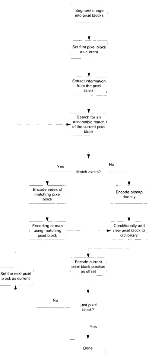
_{entry is}then copied wheneveranotherinstanceofthatcharacterappears.

JBIG2 provides for two pattern-matching algorithms, the first of which is called Pattern

Matching

and Substitution. Figure 3.13 shows the flow diagram forthe pattern _matching and

substitution algorithm. As can be seenthealgorithm starts

by

breaking

_upthe image intopixel

blocks where

hopefully

each pixel block is a character. Next each of the pixel blocks is

checked to see if it is _already in the

dictionary,

if it

is,

the index ofthe _{entry it} matches is

encoded. If it is not found in the

dictionary,

then the character is encoded and added to the

dictionary. After a pixel block is encoded its position is encoded so that the decoder knows

where toput

it,

_usuallythisposition isthe distance fromtheprevious character. Fortheactual

format ofthe JBIG2

file,

_contrary to what Figure 3.13

illustrates,

the

dictionary

data and the

encoded data (the

dictionary

index and offset) is not interleaved. The

dictionary

is kept in a

Segmentimage into pixelblocks

Set firstpixelblock as current

Extractinformation fromthepixel

block

Search foran acceptable match ofthecurrent pixel

block

No

Matchexists?

Encodeindex of matchingpixel

block

Encodebitmap

directly

Addnew pixel blockIodictionary

Setthenextpixel blockas current

, Encodecurrent pixelblockposition

as offset

T

No

Lastpixel block?

Yes

Figure 3.13- JBIG2Pattern

An algorithmforthe segmentation processdescribed above isnot given in theJBIG2 standard,

so the implementation is left _up to the programmer to use _any segmentation technique. The

next _{step in}the pattern _matching and substitutiontechnique is toextract informationabout the

pixelblock:

height,

_{width, area, position,} etc.

In a common scanned textual document two instances ofthe same character

typically

do not

matchpixel for_pixel,eventhoughthehumaneye seesthem asthesame.

Therefore,

the taskof

searching foran acceptable match inthe

dictionary

isnot atrivial one. This process is done in

two steps. The _{first step} consists ofprescreening, where each oftheentries in the

dictionary

is

checked to see if its

features, height,

_{width, area, position,} or the number ofblack pixels are

close to those ofthe current pixel block. Thesecond _step consists of_computing a match score

foreach ofthe potential matches that remain. A simple example ofthematch score wouldbe

the

Hamming

distance

[23],

which is found

by

first aligning the two blocks in comparison

accordingto theirgeometric centers oftheir

bounding

blocks andthen _counting the number of

pixelsthatdiffer. The

dictionary

_entry withthe highestmatch score isassumed tobe identical

to thepixelblock

being

encoded, if itsmatch scoreis above a predefinedthreshold.

In the case where a match is found the associated numerical

data,

the

dictionary

index and

position,areeitherbitwiseorHuffman-basedencoded. Inthecase wherethereisno acceptable

match andthenew character mustbeaddedtothe

dictionary,

the

bitmap

ofthenew characteris

encoded_usingabitonalcompressionmethod,such asG4 or

JBIG,

discussedpreviously.

Thepattern_matchingand substitutiontechnique is a

lossy

compression algorithmthatprovides

good compression ratios oftextual data. Oneproblem withthis technique isthat _occasionallya

wrong character is matched andthen when the data is

decoded,

an incorrect character exists in

thetextualdata.

The alternativeto pattern_matching and substitut