Multi-objective robust trajectory optimisation under epistemic uncertainty and imprecision

IAC–19–C1.2.1

Multi-Objective Robust Trajectory Optimisation Under Epistemic Uncertainty and

Imprecision

Sim˜ao Grac¸a Marto

_*

_,

_{Massimiliano Vasile}

_,

_{Richard Epenoy}

a

_{Department of Mechanical & Aerospace Engineering,University of Strathclyde, James Weir}

Building, 75 Montrose Street, Glasgow, United Kingdom G11XJ

,

simao.da-graca-oliveira-marto@strath.ac.uk

b

_{Centre National d’ ´}

_{Etudes Spatiales}

_{, richard.epenoy@cnes.fr}

*Corresponding Author

Abstract

This paper presents a novel method to generate robust optimal trajectories for spacecraft equipped with low-thrust propulsion under the effect of epistemic uncertainty. The uncertainties considered for this paper derive from a lack of knowledge on system’s and launcher’s parameters. This is a typical situation in the early stage of the design process when multiple options need to be evaluated and only a partial knowledge of each of them is available. Uncertainties are modelled with probability boxes, or p-boxes, embodying multiple families of distributions. Once the effect of uncertainty is propagated through the system one can calculate the Upper and Lower Expectations on the quantity of interest (for example the mass of propellant). The Lower Expectation defines the worst case effect of the uncertainty when uncertainty is expressed via a p-box. We also propose a method for its calculation, which requires solving an optimization problem. Once the low expectations on the quantities of interest are available, a novel efficient computational scheme is proposed to compute families of control laws that are robust against the effect of uncertainty. Robustness is here considered to be the ability to maximise the desired performance, under uncertainty, with a high probability of satisfying the constraints. The computational scheme proposed in this paper makes use of surrogate models of the Lower Expectations, to radically reduce the computational cost of the robust optimisation problem. This is combined with a dimensionality reduction technique, that allows one to construct surrogate models on low dimensional spaces, and an iterative refinement of the surrogate representation. The training points of the surrogate models are evaluated using FABLE (Fast Analytical Boundary value Low-thrust Estimator), an analytical tool for the fast design and optimisation of low-thrust trajectories. A memetic multi-objective optimisation algorithm, MACS (Multi Agent Collaborative Search), is then used to find the set of Pareto optimal control laws that maximise the Lower Expectation in the achievement of the desired values of objective function and constraints. The proposed approach is then applied to the design of a rendezvous mission to Apophis with a small spacecraft equipped with a low thrust engine.

Keywords:Epistemic uncertainty, Resilient satellite, Robust Optimization, Lower Expectation, Multi-Objective Optimization

Nomenclature

ξ Uncertain variable

El Lower expectation

Ξ Uncertainty space

nξ Number of uncertain variables u Control law

w Proxy variable for control law

E Expectation

Acronyms

FABLE Fast Analytical Boundary value Low-thrust Esti-mator

MACS Multi Agent Collaborative Search (optimization al-gorithm)

1. Introduction

Asteroids in the solar system are interesting targets for space exploration missions both for scientific reasons and for planetary defense. The high delta-v requirements, cou-pled with the small gravitational accelerations, make low thrust engines suited for the purpose of asteroid rendezvous. Trajectories using these engines can not be modelled as be-ing composed of instantaneous impulses, as is done with their chemical counterparts. Instead, the trajectory is split into arcs during which the engine is on or off and pointing in a certain direction. The parameters that describe these trajectories are consolidated in an arrayu(Equation 5). The challenging task of propagating and optimizing these trajec-tories is performed by FABLE, described in Section 2.

The epistemic uncertainty in the system’s and launcher’s parameters, characteristic of the early stage of the design process, provides a challenge for finding a solution that guarantees mission success under this uncertainty. Such a solution is termed robust. We will consider as uncertain variables the engine parameters at various points in the tra-jectory, as well as the Earth escape velocity provided by the launcher. One approach is to characterize this uncertainty using p-boxes, that is, a space of possible probability dis-tributions over the uncertain space. The design parameters are then optimized considering the probability distribution in this space that represents the worst case scenario. More specifically, the lower expectationElis optimized. The de-tailed definition and calculation of this quantity is the sub-ject of Section 4.

For a certain stochastic control problem, we have multi-ple metricsyi. These can be, for example, the propellant mass (mp), or the distance to a certain target (∆r). For certain thresholdsνi on these variables, we wish to find a control vectoruthat maximizes the lower expectations on each of the indicator functionsyi(u)< νi:

max

u {El(yi(u)< νi)∀i} (1)

Another interpretation forEl(yi(u)< νi)is that it repre-sents the lowest probability ofyibeing belowνithat can be obtained with the family of distributions considered. Since we’re doing a multi-objective optimization, it’s perfectly reasonable to also optimize the thresholds, so we could have:

min

u,ν{−El(yi(u)< νi); νi∀i} (2)

As shown in Section 2, the control lawuwe use has 67 dimensions. This high dimensionality is a problem given

the computational complexity of the calculation ofEl, com-bined with the multi-objective optimization. To tackle this, we use control mapping to reduce the number of dimen-sions. A variablew, with less dimensions thanu, is used as a proxy foruusing a control mapU, such that our problem becomes:

min

w,ν{−El(yi(U(w))< νi); νi∀i} (3)

Details on how that control mapping works are in Section 3. In our optimization problem we have multiple objectives, which all should be optimized in order for the mission to be likely to succeed. Sometimes optimizing one objective might conflict with optimizing another, i.e., there is a trade-off between the objectives. One way to gain knowledge of this trade-off, to assist with the design process, is to use a multi-objective optimizer to produce a Pareto front. This consists of a set of all solutions that do not dominate each other. We use MACS as a multi-objective optimizer, as well as Krigging surrogate models to speed-up convergence. This process is described in Section 5.

Our work follows a similar framework to Di Carlo et al. [1], except our method scales non-exponentially with the number of uncertain variables, we perform multi-objective optimization, and use lower expectation instead of evidence theory, among other differences.

2. Propagation and Optimization of Low Thrust Trajec-tories

The low thrust trajectories considered in this paper con-sist of an ejection by a conventional launcher, followed by a number of alternating coast and thrust arcs with ion propul-sion. The ejection is characterized by the departure timetD, and the magnitudev∞, azimuthγand declinationδof the

escape velocity relative to the Earth in a heliocentric refer-ence frame. Theithcoast arc is characterized by its length in longitude∆LOF F,i, i.e., the difference between the lon-gitude at the end of the arc and at the beginning. The ith thrust arc is characterized by its length∆LON,i, and by the azimuthαiand declinationβithat the spacecraft engine is pointing towards. Variables that are required to calculate a trajectory, but which are not part of the control vector, are the engine thrust atr = 1AU,T, and the specific impulse Isp. It is also possible to consider as control variables the throttle in each archτi, and the times of arrival at each of possibly multiple targetstT ,i, but we do not optimize these variables.

FA-BLE [2]. This uses formulas similar to those described and derived in [3], to quickly propagate using the equinoctial orbital parameters. The one difference is that we’re consid-ering a solar powered low-thrust engine, so the thrust is pro-portional to the inverse square of the heliocentric distance r:

T(r) =T1AU

2

r2 (4)

The locations of the targets at the times of rendezvous tR are calculated using a keplerian propagator. FABLE-propagator calculates the orbital parameters of the space-craft at the longitudesLRof the targets attR, as an approx-imation for the closest approach.

2.1 Optimal Trajectory

All of the variables described above, used with FABLE-propagator, define a direct transcription for the problem of optimizing a low-thrust trajectory. With FABLE [2], the user can fix some and optimize the rest of these variables. The variables that are optimized are contained in vectoru, defined as:

u= [∆LOFF∆LONα βγ δ tD] (5)

This is similar to the previous version as defined in [1], with the addition of the departure timetDas an optimisable able. We are considering 16 thrust and coast arcs, so vari-ables∆LOFF, ∆LON, α, βare each a vector with 16 el-ements, each element corresponding to each arc, for a total of 67 elements inu. It is common for arc lengths to be zero after optimization, corresponding to having a lower number of arcs in practice.

Some of the variables that are not optimized can be ei-ther fixed variables that are known a-priori, or they could be uncertain variablesξ ∈ Ξ ⊂ _Rnξ_{. FABLE can only}

opti-mize for a deterministic setting, i.e., with set values forξ, but in our work FABLE-propagator was updated to be able to quickly propagate for large numbers of differentξvalues in parallel, using CPU vectorization. This is used to quickly generate many samples of the metrics for a single control under different uncertain variables. These samples are then used with quasi-Monte Carlo methods to characterize the uncertainty in the mission objectives. This turned out to be faster than using surrogate models, as was done in [1]. The usage of these samples to characterize the uncertainty, by obtainingEl, is discussed in more detail in section 4. As an example, the uncertain variables could be:

ξ= [v∞T Isp] (6)

FABLE uses MATLAB’s fmincon to find the solution to Program 7, where the propellant mass mp is minimized, with the constraint that the spacecraft flies by or rendezvous with each target. If a target is marked as fly-by, the con-straint is that the position of the spacecraft at LRmatches that of the spacecraft, and if the target is marked as ren-dezvous, both position and velocity have to match. It is also necessary to guarantee that the spacecraft reaches this point at timetR.

min

u mp(u,ξ) s.t.∀i rf,i(u,ξ) =rT ,i

vf,i(u,ξ) =vT ,iifiis not fly-by only tf,i(u,ξ) =tT ,i

(7)

Where each i represents each target. Also, rf,i, vf,i and tf,i indicate the position, velocity and time of the space-craft when its longitude matches that of the targetiat time tT ,i. When a target is not fly-by only, the constraint that is imposed is that all equinoctial elements match, which is equivalent to requiring that the position and velocity both match.

FABLE-propagator is a tool that propagates trajectories with low-thrust engines. Its use in our work is to provide direct transcription to FABLE, and to perform Monte-Carlo analysis of the uncertainty in mission objectives.

FABLE is a tool designed to find optimal trajectories in a deterministic scenario. Its use in our work is as a way to reduce the dimensionality of the stochastic optimization problem via control mapping, as described in the next Sec-tion.

3. Control Mapping

We wish to find the control law that minimizes the lower expectation. The control law as defined in Equation 5, with 16 thrust and coast arcs, has 67 dimensions. Optimizing a nonlinear nonconvex function over such a high dimensional space would be very expensive. Instead, a control mapping strategy is used, which reduces the dimensionality of the problem, making it more suitable for use with global opti-miser and surrogate models.

withξ=ξ_u. This wayξ_uis a proxy variable for the control law. The stochastic program becomes Equation 3.

3.1 Reachable Set Mapping

In some cases we found that the above control map was too restrictive. The space of control vectors can be increased by aiming for a final position and velocity which is near, but not exactly equal, to the target’s. The displacements in both these quantities areDr andDv. Instead of usingξu as a proxy for the control vector, we usew= (ξ_u, Dr, Dv), and instead of the control map being defined by equation 7, it’s defined as:

min

u mp(u,ξu)

s.t.∀i rf,i(u,ξu) =rT ,i+Dr

vf,i(u,ξ_u) =vT ,i+Dvifiis not fly-by only tf,i(u,ξu) =tT ,i

(8)

This increases the dimensionality of our problem, enough to increase the space of solutions that we can search so as to improve our end result, but not too much that it would make the problem take too long to solve.

4. Epistemic Uncertainty

When there is epistemic uncertainty, we do not know which distribution our uncertain variablesξfollow. Multi-ple conflicting sources of information may suggest different distributions, belonging to a family. Therefore, the expec-tation of some variable can be any value within an interval bounded by the lower and the upper expectations.

We obtain robust solutions by optimizing the lower ex-pectations (El) of functions of interestI, which in our case will be defined as indicator functionsI = y < ν, repre-senting whether a metricy is below a certain thresholdν. The lower expectationElis defined as the minimum expec-tation of the function of interest with respect to a family of probability distributionsP:

El(I) = min p∈P(Ξ)

Z

Ξ

I(ξ)p(ξ) dξ (9)

We follow [4] and define the family of probability dis-tributions P using Bernstein polynomials. These Bezier curves are a linear combination of positive basis functions. If the coefficients are positive, the resulting function is guar-anteed to be positive, which makes them ideal to represent probability distributions.

We could define the family of distributions as a linear combination of multi-variate Bernstein basis functions, as in

Equation 10. This allows approximating any multi-variate distribution (see for example Section 7.4 of [5]), including those of correlated variables. The problem of finding the lower expectation is a linear program, but the complexity is exponential withnξ, as the number of coefficients is(q+ 1)nξ_{,qbeing the order of the polynomial.}

Pm=          X j∈J

cjBj(τ(ξ))

∀c>0 :X

j∈J

cj= 1

         (10)

wherej = {j1, . . . , jnξ} represents a tuple ofnξ indexes

andJ ={0, . . . , q1}×. . .×{0, . . . , qnξ} ⊂N

nξ_represents

the set of possible such tuples.

An alternative is having the distributions be the product of univariate Bernstein polynomials, as in equation 11. In this new family of distributions only independent variables are possible, since the distributions are defined as the prod-uct of univariate functions. The number of coefficients is now (q + 1)×nξ, which no longer grows exponentially with the number of uncertain variables. However, Problem 9 is no longer a linear program.

Pu=           

p(ξ;c) =

nξ Y k=1 qk X j=0

c(_jk)bj;qk(τk(ξk))

∀c>0 :X

j

c(_jk)= 1∀k

           (11)

In both of these formulas,τis a linear function such that τ(ξ) ∈ [0 1]nξ _{∀ξ ∈ Ξ. Also,b andB are Bernstein}

ba-sis functions scaled so that they’re both pdfs, that is, they integrate to 1 inΞ. Their definitions, therefore, are:

bj;q(x) = (q+ 1)

q j

xj(1−x)q−j (12)

Bi1,...,inξ;q1,...,qnξ(x) =

nξ

Y

k=1

bjk;qk(xk) (13)

whereqindicates the degree of a polynomial.

We defineE(I;c) as the expectation of I obtained by using the distributionp(ξ;c) corresponding to usingc in Equation 11:

E(I;c) =

Z

Ξ

I(ξ)p(ξ;c)dξ (14)

4.1 Estimating Expectation

Given the difficulty of calculating the integral in Equa-tion 14 analytically, a quasi-Monte Carlo approach is em-ployed. This is the same as a Monte Carlo approach, but instead of selecting the samples randomly, a deterministic, low-discrepancy sequenceξ(1), . . . ,ξ(N) is used. We use the Halton sequence for this purpose.

At this point, one way to estimate expectation E(I;c)

would be the following:

ˆ

EU(I;c) = 1

N N X

i=1

I(ξ(i))p(ξ(i);c), ξ(i)∼U (15)

Here,ξis not a random variable, but a deterministic se-quence, the Halton sequence. The expressionξ∼Umeans that the histogram ofξapproximates the pdf of distribution U, the uniform distribution. This corresponds to taking the Halton sequence as is, with no transformation. Later we will consider modifying the Halton sequence so that its his-togram is not uniform.

The Koksma-Hlawka inequality [6] provides an upper bound on the absolute error in Equation 15, but as the num-ber of dimensions increases, the upper bounds on discrep-ancy that can be found in the literature become useless, re-quiring huge (>1019_forn

ξ = 10) numbers of samples to become lower than one, which the discrepancy, by defini-tion, has to be always.

Therefore, the analysis on the error was performed using probability theory, as ifξwere randomly sampled, and af-terwards an experimental analysis was performed for a spe-cial case of indicator functions that can be easily integrated analytically.

Using probability theory, the standard deviation (σ) of Equation 15 can be written as

σ2_U = 1

N Z

I2p2dξ− Z

Ipdξ

2! ≤ 1

N Z

p2dξ,

(16)

since 0 ≤ I ≤ 1 in all domain. This expression can be calculated, given the separability of the pdf,

σ2U ≤

1

N nξ

Y

k=1

Z

(Bj(ξk))2dξk (17)

When all the weight in c is applied to thej= 0orj =q, q being the degree of the polynomials in each dimension, that upper bound becomes:

1

N

_{(q+ 1)}2

2q+ 1

nξ

(18)

which appears to be the highest value the variance can have, based on empirical results. A weightcof this type is of-ten the minimizer of the Expectation in our case. This up-per bound for the standard deviation grows exponentially with nξ. For example, if nξ = 10, q = 4and we want the standard deviation to be below 0.01, we would need N >2.7×108_samples.

To reduce the number of samples required to obtain suf-ficient accuracy, we can apply importance sampling. Impor-tance sampling is usually applied to Monte-Carlo estima-tions, but nothing logically prevents its application to quasi-Monte Carlo. It works because by changing the sampling of the variables and correcting the values of the samples appro-priately, one can obtain an estimator that is also unbiased, but which has a different, hopefully lower, variance. In our case we can haveξ ∼ P(c), henceforth referred to as “P-sampling”, whereP(c)represents the pdf obtained by using

cin Equation 11.

We obtain a sequence approximating a univariate distri-bution P with cdf C(x), if we havexu ∼ U, by doing xP = C−1(xu) ∼ P. When we have a multivariate dis-tribution of independent variables, such asP(c), ifCk(c)is the cdf along thekthvariable, we can doξk,P =C_k−1(ξk,U)

to obtain a sampling ξP ∼ P(c). This does restrict us to havingP(c)be a pdf of independent variables, but since we are using the familyPu, this is not an issue. The inverse of Ck cannot, in general, be found analytically, but very good approximations can be obtained using linear interpolation, which is what we do.

With P-sampling, the estimator becomes:

ˆ

EP(I;c) = 1

N N X

i=1

I(ξi), ξi∼P(c) (19)

σP2 =

1

N Z

I(ξ)2p(ξ)dξ−E2

≤ 1 N(E−E

2_)≤ 1

4N , (20) again using the fact that0 ≤ I ≤ 1. This new expression does not increase withnξ, solving the exponential problem we had before. Now, to obtain a similar limit on the standard deviation as before, we only need 2500 samples. We use 5000 in this document.

The fact that we now need to re-sample each time we want to evaluateE(I;c)with a differentcis a disadvantage, but, as we will see, the reduction in the number of samples evaluated for eachccompensates for the fact that they have to be recalculated for eachc. Furthermore, the number of samples required to have standard deviation below 0.01 with uniform sampling andnξ = 10,q = 4, exceeds the RAM capacity. This means that the samples would either need to be stored in hard drive or recalculated each time anyway, both of which are slower than recalculating 5000 samples.

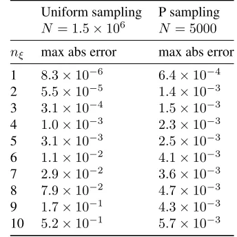
To confirm the advantage of using P-sampling, a numer-ical experiment was run. For a number of randomly gen-erated hyper-rectangular indicator functions, the exact in-tegral was calculated using analytical formulas, and esti-mated with both strategies considered here. Table 1 con-tains the maximum absolute errors with 10000 test cases obtained by comparing both estimations with the analyti-cal result. In the first column we used uniform sampling withN = 1.5×106samples, and in the second we used P sampling withN = 5000samples. The difference in the number of samples is to compensate for the fact that with P-sampling these samples will have to be calculated each time a new value ofcis considered, which is unnecessary when uniform sampling was used.

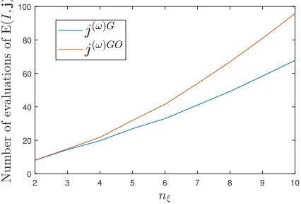
If less than300different values ofcare considered, do-ing P-sampldo-ing withN = 5000samples will be less com-putationally demanding than uniform sampling withN = 1.5×106_{. As shown in Figure 1, the algorithm evaluates}

less than300(100 per metric) differentcbefore finding a local optimum. Looking at Table 1 we see that fornξ ≥5, the error was smaller with P-sampling withN= 5000 sam-ples, and therefore, it is preferable to use this method in those cases.

4.2 Minimizing Expectation

To calculate the lower expectation we want to findcthat minimizes the expectation:

El(I) = min

c E(I;c) (21)

Table 1: Maximum absolute errors for different sampling techniques

Uniform sampling N = 1.5×106

P sampling N = 5000

nξ max abs error max abs error 1 8.3×10−6 6.4×10−4

2 5.5×10−5 1.4×10−3

3 3.1×10−4 _1.5×10−3

4 1.0×10−3 _2.3×10−3

5 3.1×10−3 2.5×10−3

6 1.1×10−2 4.1×10−3

7 2.9×10−2 3.6×10−3

8 7.9×10−2 4.7×10−3

9 1.7×10−1 4.3×10−3

10 5.2×10−1 5.7×10−3

The optimization variablechasnξ×(q+ 1)dimensions ifP =Pu, and the problem we’re optimizing is non-linear. It can be shown, however, to be equivalent to a non-linear integer problem with justnξdimensions.

Lemma 1. If El is defined using the family Pm, there is

always a vectorˆcthat only has one entry equal to 1, and all others to zero, such thatEl(I) = E(I,ˆc).

Proof. The problem of finding El withP = Pm can be written as

min

c

X

j∈J

λjcj (22)

where

λj=

Z

Ξ

I(ξ)Bj(τ(ξ))dξ (23)

This is a linear problem. Let˜jbe such thatλ˜_j= minjλj.

We can write our original problem as:

min

c λ˜j+

X

j∈J

(λj−λ˜_j)cj≥λ˜_j (24)

It’s now evident thatmincPj∈J λjcj =λ˜_j , which can

be obtained by makingc˜_j= 1andcj= 0∀j6= ˜j.

Lemma 2. If El is defined using the family Pu, there is

always a coefficient vectorˆcsuch that the lower expectation verifiesEl(I) = E(I,ˆc)withcˆsuch that:

∀k∃˜_{j: ˆc}(k) ˜

j = 1 and ˆc

(k)

Proof. We will show that if we have a vector˜csuch that

El(I) = E(I,c˜), but which does not satisfy the constraint in the lemma, we can use it to obtain a vectorˆcthat does.

If˜cdoes not satisfy that constraint, then for at least one s, we must have˜c(s)with more than one non-zero element. Let’s consider the problem of optimizingminc(s)E(I,c),

where we fix all elements ofcexcept for those inc(s). This can be written as:

min

c(s)

qs

X

j=0

λjc

(s)

j (26)

where

λη =

Z

Ξ

I(ξ)Y

k6=s qk

X

j=0

h

bj;qk(τk(ξk))˜c

(k)

j i

bη;qs(τs(ξs))dξ

(27)

This is a linear problem. Let ˜j be such that λ˜_j =

minjλj. We can write our original problem as:

min

c(s) λ˜j+

qs

X

j=0

(λj−λ˜j)c

(s)

j ≥λ˜j (28)

It is now evident thatminc(s)P

qs

j=0λjc (s)

j =λ˜j, which can be obtained by makingc(_˜s)

j = 1andc

(s)

j = 0∀j 6= ˜j. Altering˜cin this way does not change the value ofE, since

˜

cminimizedE(I,c), it must have also minimized Problem 26, and so we hadPqs

j=0λj˜c (s)

j =λ˜j

By repeating this process for allsfor whichc(s)_{has more}

than one non-zero element, we obtain a new vectorˆcfor which the condition in the lemma is satisfied, and for which

E(I,ˆc) = E(I,˜c) = El(I).

These lemmas tell us that regardless of which family of pdfs,Pmor Pu, we use in Program 9 to calculateEl, the value we get could be obtained by using one of the multi-variate Berstein basis distributions. Therefore, using either of those families is equivalent to using the following discrete set:

Pj ={Bj(τ(ξ))∀j∈ J ⊂Nnξ} (29)

This allows us to reformulate our problem as the follow-ing integer problem:

El(I) = min

j∈J E(I;j) (30)

where,

E(I;j) =

Z

Ξ

I(ξ)Y

k

Bj(k)(τk(ξk))dξ (31)

This reduces our search space to justnξdimensions, and will be the basis for the minimization algorithm we propose.

4.3 Minimization Algorithm

Since it is our requirement that the execution time of the algorithm is polynomial with the number of dimensions, go-ing through each possible combination of indexes is out of question. Instead, a method similar to a pattern search is employed. This method, at each step, finds the mutation jk = x that most reduces the value ofE, as in Equation 32. At each step there is a guarantee that the value ofEis decreased. These steps are repeated until no improvements can be made.

argmin

ˆ

k,x

EI;j(t+1)

j(_ˆt+1) k =x

j_k(t+1)=j_k(t)∀k6= ˆk

(32)

Note that when we calculate one metricyiwe also calcu-late all the other metrics, because all metrics require propa-gating the trajectory, which is where most of the execution time is spent. This means that when we calculate an expec-tationE(yi < νi;c)we also calculate the expectations for the other metrics. To reduce execution time, memoization is applied, i.e., when we evaluateE(yi < νi;c), we store

E(yj< νj;c)∀jin case these values are needed in the esti-mations ofEl(yj< νj).

The process in Equation 32 always finds a local solution, but has no guarantee of finding the global optimum. The solution returned by this method depends on the initial guess

j(0)_.

One possible initial guess is to choose greedily eachjk, according to:

∀k, j_k(0)G= argmin

i Z

Ξ

I(ξ)bi,q_k(ξk)dξ (33)

The solution obtained using this initial guess will be termed j(ω)G_{. To improve the likelihood of finding the} optimal solution, we re-start the optimization with a new initial guess. We want this initial guess to be unlikely to fall into the same local optimum asj(ω)G_{, so we define it,}

34. The solution obtained by applying the pattern search starting fromj(0)GO _{is compared withj}(ω)G_{, and the one} which produces the lowest value of the expectation is kept and termedj(ω)GO_.

j(0)_k GO=qk−j(_kω)G (34)

Experimental Results

To assess the accuracy of this algorithm, an experiment was performed. Fornξranging from 2 to 10, 1667 different values ofwwere sampled following the Halton sequence. For each of those, 3 indicator functions were created, one for each of the 3 metrics used in the test case in Section 6.1: pro-pellant mass, distance and relative speed to target (Apophis). This produces 5001 different indicator functions, for each of which both versions of the algorithm were run. Fornξ up to 5, the solution was obtained using a brute-force method, to obtain error metrics. For highernξ, it was too time con-suming to perform brute-force search. Table 2 shows the maximum absolute errors of the algorithm with and without the new starting point, and Table 3 shows the fraction of the errors that were below10−6.

Table 2: Maximum absolute error betweenEl(obtained by brute-force search) andEobtained using either of the algo-rithms considered.

nξ j(ω)G _j(ω)GO

2 0 0

3 0.0151 0 4 0.1046 0 5 0.1513 0.0001

Table 3: Percentage of absolute errors below10−6. Abso-lute error betweenEl(obtained by brute-force search) andE obtained using either of the algorithms considered.

nξ j(ω)G _j(ω)GO

2 100% 100%

3 99.8% 100%

4 97.3% 99.98% 5 97.5% 99.96%

In Figure 1 we can see the number of different values ofj that are evaluated, on average, per indicator function. Note that this number has been reduced thanks to memoiza-tion as menmemoiza-tioned previously. For either of the algorithms,

the number of function evaluations remains under 100 per indicator function.

2 3 4 5 6 7 8 9 10

0 20 40 60 80 100

Fig. 1: Number of function evaluations per indicator func-tion for which the lower expectafunc-tion is to be calculated.

Given these results, we will be usingj(ω)GO_{to calculate}

El.

5. Multi Objective Optimization of Lower Expectation

Oftentimes the optimization of one objective conflicts with the optimization of another. It is not always possible to determine how to weigh each of them so as to obtain a unique solution. A solution is said to be dominated if there’s a point in the search space that is better than it in every ob-jective. Naturally, regardless of the importance the design-ers give to each of the objectives, they will always prefer to choose a non-dominated solution. Therefore, when we have a multi-objective problem, we wish to estimate the Pareto front, which is the set of all non-dominated solutions. A tool that obtains samples that approximate the Pareto front is called a multi-objective optimizer. We’re using MACS for this purpose.

5.1 Surrogate Models

In our work we employ Kriging models E˜l, using the DACE toolbox [8], to speed-up the optimization. These try to capture the relationship betweenw, νandEl(I(yi< νi)). One model is trained to approximate the lower expectation for each metric:

˜

El i(w, νi)≈El(I(yi(U(w))< νi)) (35)

At the start of our method, the proxy control variable wand the thresholdsν are sampled with 100 elements of the Halton sequence, and for each of those we calculate

El(I(yi(U(w)) < νi). The Kriging model is then trained to fit the values of the lower expectation.

MACS is then called on these models, and the lower ex-pectations for the solutions it returns are calculated accu-rately. These values are then introduced in the model, which is then re-trained, and this process is repeated several times. This part of the process is necessary because the model is imperfect and the optimizer might find points that are poorly represented in the model and which appear to be good so-lutions because of it. This approach also leads to a higher sampling rate where it matters most - near the Pareto front.

We use a Kriging model with linear regression func-tions, and exponential correlation functions. We found that the choice of the correlation model is critical to ensure the model converges.

Each time MACS is run, the points that it finds are in the Pareto set, which is a subset of the search space. Using Gaussians as correlation functions, when too many training points are added in a subset of the search space, the model diverges. The accuracy of the model at points distant from this subset worsen considerably. This does not happen with exponential correlation functions, which are more “local” in the sense that adding training points in one region of the set does not affect significantly the value of the model in distant points.

MACS is run with 10000 function evaluations and an archival size of 10 and population of 21 agents during 10 iterations of refining the model. Afterwards, it’s run once on the final model with 252 agents and 100 elements in the archive with 100000 function evaluations. The archive at the end of running MACS contains the solutions, and in our case it was always full. All of these solutions are then used to refine the model.

6. Test Cases : Rendezvous with Apophis

We consider two test cases. In both of them we study a rendezvous mission with Apophis, but we consider two

different formulations for uncertainty. In the first, we have uncertain engine parameters, and in the second we have un-certain engine outage.

Apophis is an asteroid that in 2004 was classified as level 4 in the Torino scale, the highest ever score, due to a prob-ability of impact that reached 1 in 60 at its highest estimate [9]. Later information lead to this probability becoming practically 0, and the asteroid being reclassified as level 0 in Torino scale, indicating that it poses no threat. Nonethe-less its orbit regularly intersects the Earth’s, and on average it passes within two lunar orbits every five years [9].

This makes it an excellent test case for robust design of asteroid rendezvous missions, with the purpose of improv-ing predictions about future approaches or even redirect it if ever necessary. For such missions it is important to guar-antee that the objectives are met in the face of significant epistemic uncertainty.

We consider the robust optimization of a mission with a spacecraft equipped with an ion engine with uncertain en-gine parameters and Earth escape velocity. The orbital ele-ments for Apophis, for the epoch 28 September 2008, were taken from the JPL small object database∗.

The metricsyconsidered were the propellant mass spent mp, the distance to target∆rand the relative speed to target

∆vat rendezvous. We are running MACS to optimize the surrogate models of the lower expectations on these quanti-ties. The thresholds for these quantities were also optimized simultaneously with the other quantities, as in Equation 2. Therefore, our optimization problems can be written as:

min

w,ν

−E˜l mp(w, νmp)

−E˜l∆r(w, ν∆r) −E˜l∆v(w, ν∆v)

νmp

ν∆r ν∆v

(36)

The difference between the two test cases considered here is only on the definition ofξ.

6.1 Uncertain Engine Parameters

We considered the engine thrust and Isp to vary with lon-gitude in a way that is uncertain. This is modelled with un-certain variablesTiandIsp,irepresenting the value of these parameters at equispaced longitudes. The values at interme-diate longitudes are obtained by linear interpolation. The Earth escape velocityv∞was also considered uncertain.

Therefore, variableξis given as

Table 4: Lower and upper bounds that defineΞ, the hyper-rectangular space of uncertain variables, for the uncertain en-gine parameters test case.

v∞[Km/s] Ti[N] Isp,i[s]

ξL 3 2772 0.0477

ξU 3.7 3388 0.0583

ξ= [v∞T1 · · · TnT Isp,1 · · · Isp,nI] (37)

We considerednT = 5andnI = 4so thatnξ = 10. This number was chosen to demonstrate the ability of our method to deal with high numbers of epistemic uncertain variables. The uncertain variables are bounded according to Table 4, whereξLandξU represent the lower and upper bounds, such thatΞ =hξLξUi.

Results

In Table 5 are shown a selection of solutions found by this method. To visualize the nature of the trade-offs, a Pareto front with fixed thresholds was obtained, which is shown in Figure 2.

Fig. 2: Scatter plot of Pareto front for lower expectations with fixed thresholds. The values of the thresholdsνmp,ν∆r

andν∆vare45Kg,0.018AU and0.7Km/s, respectively. The colors indicateEl mprop< νmprop

.

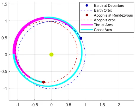
As an illustration, the seventh row solution from Table 5 was plotted for 200 differentξ values to produce a line

Table 5: A selection of solutions returned by our method. Solutions were selected using the same archival algorithm employed by MACS, after solutions withEl ≤ 0.01were removed.

Elm El∆r El∆v νm[Kg] ν∆r[AU] ν∆v[Km/s]

0.690 1.000 1.000 50.797 0.041 2.099 1.000 1.000 1.000 52.169 0.042 2.155 1.000 0.062 1.000 79.476 0.023 3.655 1.000 1.000 0.153 80.517 0.066 0.764 1.000 0.698 0.581 80.605 0.021 0.792 1.000 0.447 1.000 52.282 0.026 0.939 1.000 1.000 0.745 52.070 0.067 0.673 0.848 0.797 1.000 45.168 0.024 3.627 1.000 0.309 1.000 52.178 0.027 3.614 1.000 1.000 0.921 81.000 0.029 0.943

whose thickness can serve as a visualization of the uncer-tainty in position (Figure 3).

Fig. 3: Plot of trajectories for the control law corresponding to the last solution in Table 5 and for 200 different samples of

ξ, so that the thickness can serve to visualize the uncertainty in position. The plot is seen perpendicularly to the ecliptic plane and the axis are in AU.

6.2 Engine Outage

A different type of unexpected engine behaviour is an en-gine outage. In our case we considered as random variables the location of the beginning of the outageLO, its duration

Table 6: Lower and upper bounds that defineΞ, the hyper-rectangular space of uncertain variables, for the engine out-age test case.

v∞[Km/s] LO[rad] ∆LO[rad] ηO

ξL 3 0 0 0

ξU 3.7 4π π/8 1.2

without the outage, becomesηOT. We still considerv∞as

an uncertain variable.

The uncertain vectorξfor this test case is given as

ξ= [v∞LO∆LOηO] (38)

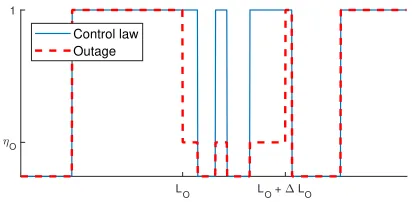
As an example of engine outage being applied to a con-trol vector consider the case illustrated in Figure 4. The curves represents the engine thrust as a fraction of its maxi-mum value, with and without the effect of outage.

L_O L_O + L_O

O

1

Control law Outage

Fig. 4: Example of the effect of engine outage as modelled in this work. Both lines represent the fraction of maximum available thrust as a function of the longitude. The blue solid line represents this fraction as specified by the control vector, and the red dashed line is the thrust that is actually applied due to the outage.

The bounds forξfor this test case are represented in Ta-ble 6.

Results

Once again we obtain a table with a selection of solutions returned by our method, in Table 7, and a plot for many values ofξ∈Ξin Figure 5. Running the optimization with fixed thresholds produces a3D plot as the one in Figure 6.

Table 7: A selection of solutions returned by our method. Solutions were selected using the same archival algorithm employed by MACS, after solutions withEl ≤ 0.01were removed.

Elm El∆r El∆v νm[Kg] ν∆r[AU] ν∆v[Km/s]

0.113 0.431 0.432 33.968 0.023 1.205 0.121 0.383 0.385 36.581 0.025 1.298 1.000 1.000 1.000 44.588 0.009 3.524 1.000 1.000 0.089 60.265 0.020 0.283 0.110 1.000 1.000 28.911 0.065 2.968 1.000 0.328 1.000 76.775 0.009 3.598 1.000 0.269 0.261 44.370 0.064 0.692 0.262 0.058 1.000 41.975 0.007 3.432 0.290 1.000 0.137 41.891 0.018 0.558 1.000 1.000 0.548 70.717 0.027 0.653

Fig. 5: Plot of trajectories for the control law corresponding to the last solution in Table 7 and for 200 different samples of

Fig. 6: Scatter plot of Pareto front for lower expectations with fixed thresholds. The values of the thresholdsνmp,ν∆r

andν∆v are 35Kg, 0.005AU and 0.75Km/s, respectively. The colors indicateEl(∆r < ν∆r).

6.3 Execution Times

The execution time can be split into three parts, the com-putation ofEl and the control map, to create the training points for the surrogate model, and running MACS on the surrogate model. The following times were obtained in Matlab(R) 2018b on a Windows 10 computer with Intel(R) Core(TM) i7-8700 @3.2GHz and 8GB of RAM.

• Running MACS on the surrogate model takes about 10 seconds per iteration with 10000 function evaluations, and 40 seconds for the final iteration with 100000. • The control map (Problem 8) takes about 3.7 seconds,

to calculateufromw.

• Solving Problem 30 to obtainElfromutook 4.5 sec-onds for the first test case (variable thrust and Isp) and 7.7 seconds for the second (engine outage). The longer time with engine outage is because the calcu-lation of the values of the indicator function for the quasi-Monte-Carlo estimation ofE(I;c)could not be fully vectorized.

There are in total 300 points for which we calculateEl, 100 for the initial surrogate, 10 per iteration and 100 for the final iteration. In total, the first test case took 45 minutes and the second 1 hour, approximately.

7. Conclusions

This paper has presented a method for obtaining robust solutions for the optimal control problem of finding a

tra-jectory to rendezvous with an asteroid. The uncertainty was modelled using lower expectation, a method which allows taking into account epistemic uncertainty. The family of distributions used to define the lower expectation was based on Bernstein polynomials.

A method to solve the optimisation problem required to calculate lower expectation without exponential complexity on the number of uncertain variables was also developed.

We applied our method to two test cases, both of which consider a rendezvous mission with asteroid Apophis. The first considered an engine with unknown parameters, which evolve over time in an unknown way. The second applied this process to an engine outage, where for a small amount of time, the engine’s thrust suddenly changes in an unpre-dictable way.

This method could be applied to any design problem sub-ject to epistemic uncertainty with multiple possibly conflict-ing objectives. As future work we will apply this method to a trajectory with more than one target, such as an asteroid tour.

Acknowledgement

This research has been developed with the partial sup-port of the CNES grant R-S17/BS-0005-034 ”Robust Op-timization of Low-Thrust Interplanetary Trajectories” and the H2020 MCSA ITN UTOPIAE grant agreement number 722734.

References

[1] Marilena Di Carlo and Massimiliano Vasile. “Robust Optimisation of Low-Thrust Interplanetary Transfers Using Evidence Theory”. In: AAS/AIAA Space Flight Mechanics Meeting. Jan. 13, 2019.

[2] Marilena Di Carlo, Juan Manuel Romero Martin, and Massimiliano Vasile. “CAMELOT: Computational-Analytical Multi-fidElity Low-thrust Optimisation Toolbox”. In: CEAS Space Journal 10.1 (Mar. 1, 2018), pp. 25–36.ISSN: 1868-2510.DOI:10.1007/ s12567 - 017 - 0172 - 6.URL:https : / / doi .

org/10.1007/s12567- 017- 0172- 6(visited

on 01/25/2019).

[3] Federico Zuiani and Massimiliano Vasile. “Extended analytical formulas for the perturbed Keplerian mo-tion under a constant control acceleramo-tion”. In: Ce-lestial Mechanics and Dynamical Astronomy 121.3 (Mar. 1, 2015), pp. 275–300. ISSN: 1572-9478. DOI:

//doi.org/10.1007/s10569- 014- 9600- 5

(visited on 04/12/2019).

[4] Massimiliano Vasile and Chiara Tardioli. “On the Use of Positive Polynomials for the Estimation of Upper and Lower Expectations in Orbital Dynamics”. In:

Stardust Final Conference (2018), pp. 99–107. DOI:

10 . 1007 / 978 - 3 - 319 - 69956 - 1 _ 6. URL:

https : / / link . springer . com / chapter / 10.1007/978- 3- 319- 69956- 1_6(visited on 03/05/2019).

[5] Clemens Heitzinger. “Simulation and Inverse Model-ing of Semiconductor ManufacturModel-ing Processes”. dis-sertation. Technischen Universit¨at Wien, Nov. 2002. [6] Harald Niederreiter.Random number generation and

quasi-Monte Carlo methods. en. CBMS-NSF regional conference series in applied mathematics 63. Philadel-phia, Pa: Society for Industrial and Applied Mathemat-ics, 1992.ISBN: 978-0-89871-295-7.

[7] Lorenzo A. Ricciardi and Massimiliano Vasile. “Im-proved Archiving and Search Strategies for Multi Agent Collaborative Search”. In:Advances in Evolu-tionary and Deterministic Methods for Design, Opti-mization and Control in Engineering and Sciences. Ed. by Edmondo Minisci et al. Computational Methods in Applied Sciences. Cham: Springer International Pub-lishing, 2019, pp. 435–455.ISBN: 978-3-319-89988-6.

DOI:10.1007/978-3-319-89988-6_26.URL:

https://doi.org/10.1007/978- 3- 319-89988-6_26(visited on 01/25/2019).

[8] H. B. Nielsen, S. N. Lophaven, and J. Søndergaard.

DACE - A Matlab Kriging Toolbox. Richard Petersens Plads, Building 321, DK-2800 Kgs. Lyngby, 2002. URL: http : / / www2 . imm . dtu . dk / pubdb / views / publication _ details . php ? id = 1460.

[9] Don Yeomans, Steve Chesley, and Paul Chodas. Near-Earth Asteroid 2004 MN4 Reaches Highest Score To Date On Hazard Scale. 2004. URL: https : / / cneos.jpl.nasa.gov/news/news146.html