City, University of London Institutional Repository
Citation:
Wang, Jinghua (2016). A hybrid model for large scale simulation of unsteady nonlinear waves. (Unpublished Doctoral thesis, City University London)This is the accepted version of the paper.
This version of the publication may differ from the final published
version.
Permanent repository link:
http://openaccess.city.ac.uk/14575/Link to published version:
Copyright and reuse: City Research Online aims to make research
outputs of City, University of London available to a wider audience.
Copyright and Moral Rights remain with the author(s) and/or copyright
holders. URLs from City Research Online may be freely distributed and
linked to.
City Research Online: http://openaccess.city.ac.uk/ [email protected]
1
A HYBRID MODEL FOR LARGE SCALE
SIMULATION OF UNSTEADY NONLINEAR WAVES
By
Jinghua Wang
B. Eng.
Supervisor
Prof. Qingwei Ma
A thesis submitted to
City University London
for the degree of
Doctor of Philosophy
School of Mathematics, Computer Science and Engineering
City University London
2
CONTENTS
LIST OF FIGURES ... 5
LIST OF TABLES ... 8
ACKNOWLEDGEMENTS ... 9
DECLARATION ... 10
ABSTRACT ... 11
LIST OF SYMBOLS AND TECHNICAL TERMS ... 12
1 INTRODUCTION ... 18
2 LITERATURE REVIEW ... 22
2.1 Steady wave models ... 22
2.1.1 Linear wave model ... 23
2.1.2 Stokes wave model... 23
2.1.3 Shallow water wave models ... 24
2.1.4 Suitability of steady wave models ... 25
2.2 Unsteady wave models ... 26
2.2.1 Second order wave models ... 26
2.2.2 Shallow water wave models ... 29
2.2.3 Nonlinear Schrödinger equations ... 32
2.2.4 Fully nonlinear models ... 36
2.2.5 Potential-NS models ... 41
2.3 Existing problems, objectives and main contribution ... 42
2.4 Outline of the thesis ... 44
3 MATHEMATICAL FORMULATIONS AND PREVIOUS WORKS ... 45
3.1 The fundamental equations ... 45
3.2 The Enhanced Nonlinear Schrödinger equation ... 46
3.2.1 Governing equation for the free surface envelope ... 47
3.2.2 Solution to the free surface and velocity potential ... 49
3.3 The Higher Order Dysthe equation ... 49
3.3.1 Governing equation for the free surface envelope ... 49
3.3.2 The fifth order ENLSE based on Hilbert transform ... 50
3.4 The Spectral Boundary Integral method ... 51
3.4.1 The prognostic equations ... 51
3.4.2 The boundary integral equation ... 52
3.4.3 Numerical implementation ... 54
3
3.4.5 Quasi SBI ... 57
3.5 Discussion ... 58
4 THE FIFTH ORDER ENLSE BASED ON FOURIER TRANSFORM ... 59
4.1 The governing equation for the free surface envelope ... 59
4.2 Numerical implementation ... 60
4.3 Validation of the ENLSE-5F ... 61
4.4 Discussion ... 64
5 THE ENHANCED SPECTRAL BOUNDARY INTEGRAL METHOD ... 66
5.1 Techniques for de-singularity ... 66
5.1.1 Weak-singular integral in 𝑉4 ... 66
5.1.2 Weak-singular integral in 𝑉3 ... 67
5.1.3 Effectiveness of the de-singular techniques for evaluating 𝑉3 and 𝑉4 ... 68
5.2 Techniques for Anti-Aliasing (TAA) ... 75
5.2.1 Anti-aliasing Techniques ... 76
5.2.2 Comparisons of different anti-aliasing techniques ... 82
5.3 Techniques for determining the critical surface slope ... 84
5.3.1 Estimation of magnitude of 𝐷𝑐 ... 85
5.3.2 Values of 𝐷𝑐 determined by numerical tests ... 85
5.4 Overall efficiency of the ESBI ... 89
5.5 Discussion ... 93
6 THE HYBRID MODEL ... 94
6.1 Relationship between 𝜂 and 𝐴 ... 95
6.1.1 Transformation from 𝐴 to 𝜂 and 𝜙 ... 95
6.1.2 Transformation from 𝜂 to 𝐴 ... 96
6.2 Methodology for the timing control ... 97
6.3 Effects of 𝑇𝑜𝑙1 and 𝑇𝑜𝑙2 by numerical simulations ... 99
6.3.1 Investigation on effects of 𝑇𝑜𝑙2 ... 101
6.3.2 Investigation on effects of 𝑇𝑜𝑙1 ... 103
6.4 Validation of the hybrid model ... 105
6.4.1 Two dimensional simulations ... 105
6.4.2 Three dimensional simulations ... 108
6.5 Discussion ... 113
7 NUMERICAL SIMULATION OF ROGUE WAVES IN RANDOM SEAS ... 114
7.1 Techniques to embed rogue waves ... 114
7.1.1 Basic formulations ... 114
4
7.1.3 Discussion ... 121
7.2 Discussions on the overall performance of the hybrid model ... 122
7.2.1 Different rogue wave height ... 122
7.2.2 Different numbers of rogue waves on temporal scale ... 126
7.2.3 Different numbers of rogue waves on space scale ... 131
7.3 Discussion ... 136
8 CONCLUSIONS AND RECOMMENDATIONS ... 137
8.1 Conclusions ... 137
8.2 Recommendations ... 138
APPENDIX A ... 141
APPENDIX B ... 146
APPENDIX C ... 148
APPENDIX D ... 149
APPENDIX E ... 152
5
LIST OF FIGURES
Figure 3.0.1 Sketch of the problem ...45
Figure 3.2.1 Sketch of the envelope ... 47
Figure 3.4.1 Flow chart for the numerical implementation of Spectral Boundary Integral Method ... 55
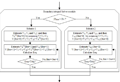
Figure 3.4.2 The flow chart of the numerical scheme for solving the boundary integral equation ... 57
Figure 4.2.1 Flow chart for the numerical implementation of ENLSE-5F ... 61
Figure 4.3.1 Profiles of Ψ2 and Ψ3 ... 62
Figure 4.3.2 Envelopes of the numerical simulations ... 63
Figure 4.3.3 Profiles of the free surface ... 64
Figure 5.1.1 The local polar coordinates for the elements near the singular point ... 67
Figure 5.1.2 Profiles of V3 and V4 ... 70
Figure 5.1.3 Relative error of the profiles of V3(a) and V4(b) ... 71
Figure 5.1.4 Profiles of the free surfaces ... 73
Figure 5.1.5 Variation of the phase shift of wave profiles with time ... 74
Figure 5.1.6 Results for the case with a domain of 2𝐿 × 2𝐿 and 𝜀 = 0.2985 ... 75
Figure 5.1.7 Resolution and CPU ratio to achieve 𝐸𝑟𝑟1< 2.5% for different values of steepness ... 75
Figure 5.2.1Illustration of TAA1 ... 78
Figure 5.2.2 Illustration of TAA2 ... 79
Figure 5.2.3 Profiles of V4(2) ... 80
Figure 5.2.4 Illustration of TAA3 ... 81
Figure 5.2.5 Aliasing error against different resolutions for different steepness ... 83
Figure 5.2.6 Resolution and CPU ratio to achieve 𝐸𝑟𝑟𝑜𝑟{𝑉3+ 𝑉4} < 1𝐸 − 6 for different values of steepness ... 83
Figure 5.3.1 Ratio of CPU time taken by Scheme 1 to that of Scheme 2 for Err1{𝜑} < 2.5% ... 84
Figure 5.3.2 Wave profiles at different instants (a) and numerical error against maximum gradient (b) for 𝑝0= 0.25 ... 87
6
Figure 5.3.5 Results for horse-shoe wave pattern ... 88
Figure 5.4.1Evolution of perturbation components of𝑲 = (3/2, 4/3) ... 90
Figure 5.4.2 Free surface profiles at different section for𝜀 = 0.3at𝑇/𝑇0= 18 ... 91
Figure 5.4.3 Convergent rate of Fructus method and ESBI for 𝜀 = 0.1, 0.2 and 0.3... 92
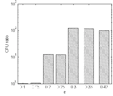
Figure 5.4.4 CPU time ratio against steepness at error less than 0.2% ... 92
Figure 5.4.5 Profiles corresponding to different errors for𝜀 = 0.3at𝑇/𝑇0= 18 ... 93
Figure 6.1.1 Flow chart of estimating the envelope 𝐴 by iterations ... 97
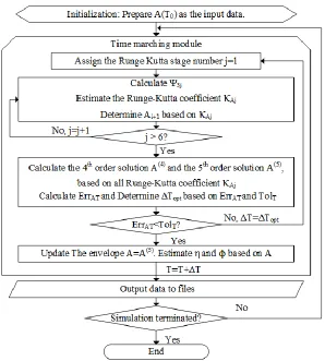
Figure 6.2.1Flow chart of the numerical scheme for hybrid model ... 99
Figure 6.3.1𝐸𝑟𝑟𝜂 against𝑇𝑜𝑙2 ... 102
Figure 6.3.2 𝐸𝑟𝑟𝜂 against 𝑇𝑜𝑙1 ... 104
Figure 6.4.1 Free surface at the end of the simulation. ... 105
Figure 6.4.2 The exchange between the models ... 106
Figure 6.4.3 Free surface at different instant. ... 107
Figure 6.4.4 The exchange between the models ... 108
Figure 6.4.5 The Profiles of free surface at 𝑇/𝑇0= 7.4 for focusing wave ... 109
Figure 6.4.6 The exchange between the models for focusing wave ... 109
Figure 6.4.7 Evolution of perturbation components and peak wave components crescent wave ... 110
Figure 6.4.8 The exchange between the models for crescent wave ... 111
Figure 6.4.9 Free surface elevation at 𝑇/𝑇0= 250 ... 112
Figure 6.4.10 Probability distribution of the free surface elevation at 𝑇/𝑇0= 200 ... 112
Figure 7.1.1 Free surface and observed spectra based on the JONSWAP spectrum. ... 118
Figure 7.1.2 Observed spectra based on the JONSWAP spectrum ... 118
Figure 7.1.3 Free surface and observed spectra based on the Gaussian distribution. ... 119
Figure 7.1.4 Free surface and observed spectra based on the CNW. ... 120
Figure 7.1.5 Free surface and observed spectra for multiple rogue waves tests. ... 121
Figure 7.2.1 𝐸𝑟𝑟𝜂 and CPU ratio (CPU time of ESBI/CPU time of hybrid model) for the cases with different rogue wave heights ... 123
Figure 7.2.2 The exchange between models for the cases with different rogue wave heights ... 126
7
Figure 7.2.4 𝐸𝑟𝑟𝜂 and CPU ratio (CPU time of ESBI/CPU time of hybrid model) : different
rogue wave number on temporal scale ... 127 Figure 7.2.5 Maximum wave elevations with indicator which model is used for the cases of different numbers of rogue waves in time domain ... 129
Figure 7.2.6 The profiles of the rogue waves for the cases of different numbers of rogue waves in time domain ... 130
Figure 7.2.7 𝐸𝑟𝑟𝜂 and CPU ratio (CPU time of ESBI/CPU time of hybrid model) for the
cases of different amount of rogue waves on spatial scale ... 131 Figure 7.2.8 Maximum wave elevations with indicator which model is used for the cases of different numbers of rogue waves in spatial domain ... 134
8
LIST OF TABLES
9
ACKNOWLEDGEMENTS
I would like to show my gratitude to all the people who have spent their precious time and offered me kind helps during my postgraduate study. Without their supports, this thesis cannot be made possible.
Firstly, I must express the sincerest appreciation to my supervisor, Prof. Qingwei Ma, who is the most influential person throughout my postgraduate study. He has inspired me in so many ways, and I’ve learnt a lot from our numerous discussions. I am so impressed by his profound knowledge and keen enthusiasm for researches and patience for educating his students. He has taught me valuable research skills that benefit not only my study, but also my careers in the future. He always encourages and pushes me to overcome one challenge after another, which enables me to know better about myself, dig my potential and gain confidence again and again. I will always remember his rigorous style of supervising, which will endeavor me to make further progress as a researcher.
I am also indebted to Dr. Shiqiang Yan, who has given me so much enlightening ideas and useful suggestions during my study. He also generously offered me his numerical code, without which my research won’t be that smooth.
I am thankful to Prof. Huajun Li, who had supervised me during my master study at Ocean University of China and introduced me to Prof. Ma. I would also like to show my thanks to Prof. Bingchen Liang and Prof. Dongyoung Lee, who also provided kind helps during my PhD study. Thanks to all my friends, with whom I have spent a very joyful and meaningful four-year, and that I will never forget.
I also appreciate the sponsorship provided by China Scholarship Council for the first 48 months and the last 4 months by Prof. Qingwei Ma during my study.
10
DECLARATION
No portion of the work referred to in the thesis has been submitted in support of an application for other degree or qualification of this or any other university or other institute of learning.
11
ABSTRACT
12
LIST OF SYMBOLS AND TECHNICAL TERMS
𝑇0 Peak period, characteristic period, Stokes wave period
𝐿0 Peak wave length, characteristic wave length
𝑘0 Peak wave number, characteristic wave number
𝑏 Draught of the cylinder
ℎ Water depth
𝑈𝑟 Ursell number
𝑎 Wave amplitude
k Wave number
ε Wave steepness
𝜂 Free surface elevation
∆ Laplacian
𝜙 Velocity potential
𝑝 Pressure on free surface
𝑿 Horizontal coordinates
𝑋 Transversal coordinate
𝑌 Longitudinal coordinate
𝑍 Vertical coordinate
𝑇 Time coordinate
𝜔0 Peak circular frequency
𝜌 Density of water
𝑔 Gravitational acceleration
𝐹{ } Fourier transform
𝐹−1{ } Inverse Fourier transform
𝑲 Variable wave number corresponding to 𝑿
𝜅 Transversal wave number corresponding to 𝑋
𝜁 Longitudinal wave number corresponding to 𝑌
𝑎𝑗 Wave amplitude of the jth component
𝒌𝒋 Wave number of the jth component
𝜔𝑗 Circular frequency of the jth component
13
𝑖 Imaginary unit
𝐴 Envelope of the free surface elevation
𝐵 Envelope of the velocity potential
𝐴𝑗 The 𝑗𝑡ℎ harmonic coefficients for free surface elevation
𝐵𝑗 The 𝑗𝑡ℎ harmonic coefficients for velocity potential
𝜂̅ Free surface deflection due to wave radiation stress
𝜙̅ Mean flow due to wave radiation stress
𝑐. 𝑐. Complex conjugate
𝜃 Phase of the harmonic
𝓌 Circular frequency of envelope
𝒌𝟎 Directional peak wave number
Ψ1 Nonlinear part of the ENLSE-4
Υ1 Nonlinear part excluding the mean flow term of the ENLSE-4
Ψ2 Nonlinear part of the ENLSE-5H
Υ2 Nonlinear part excluding the Hilbert transform terms and Υ1 of the
ENLSE-5H
ℋ{ } Hilbert transform of first kind
𝒫{ } Hilbert transform of second kind
𝜙̃ Velocity potential at free surface
𝑉 Vertical velocity at free surface
𝑴 Vector form of the variables for free surface and velocity potential
𝒜 Matrix form of the circular frequency
𝑹 Vector form of the pressure term on free surface boundaries
𝑵 Vector form of the nonlinear parts of the free surface boundary
conditions
𝛺 Variable circular frequency
𝐾 Module of variable wave number
∆𝑇 Time step
𝛼𝑗, 𝛽𝑗 Six-stage embedded fifth order Runge-Kutta coefficients
𝒦𝑗 Runge-Kutta increment at each stage
𝐸𝑟𝑟𝑇, 𝑇𝑜𝑙𝑇 Relative error between the fourth order and fifth order Runge-Kutta
solutions and the tolerance
∆𝑇𝑜𝑝𝑡 Optimised time step size
14
𝑟 Distance between the source and field point
𝑹 Vector pointing from source to field point
𝑅 Module of 𝑹
𝒏 Unit normal vector on free surface pointing outside
𝑆0 projection of 𝑆 to the horizontal plane
𝐷 Difference of the free surface between source and field point over their horizontal distance
𝑉𝑗 The 𝑗𝑡ℎ order convolution of the vertical velocity
Γ1 Kernel of the integration part of 𝑉3
Υ1 Kernel of the integration part of 𝑉4
𝑉4(1) The third order convolution part of 𝑉4
𝑉4,𝐼′ The integration part of 𝑉4 up to the fifth order
𝑉𝐼𝑡𝑒𝑟, 𝑉𝐼𝑡𝑒𝑟+1 The values of the velocity 𝑉 at two successive iterations
𝐸𝑟𝑟𝐵, 𝑇𝑜𝑙𝐵 Relative error between 𝑉𝐼𝑡𝑒𝑟 and 𝑉𝐼𝑡𝑒𝑟+1, and the tolerance
∆𝑿 Spatial step size
𝑉3(1) The fourth order convolution part of 𝑉3
𝑉3(2) The sixth order convolution part of 𝑉3
𝑉3,𝐶 The whole convolution part of 𝑉3
𝑉3,𝐼 The integration part of 𝑉3 up to the eighth order
𝑉4(2) The fifth order convolution part of 𝑉4
𝑉4(3) The seventh order convolution part of 𝑉4
𝑉4,𝐶 The whole convolution part of 𝑉4
𝑉4,𝐼 The integration part of 𝑉4 up to the ninth order
Γ2, Υ2 New kernel of the integration part of 𝑉3 and 𝑉4 respectively after further
expansion
𝐷𝑐 Critical value of 𝐷
|𝐷|𝑚𝑎𝑥 Maximum value of the module of 𝐷
Ψ3 Nonlinear part of the ENLSE-5F
𝐴(4), 𝐴(5) Fourth and fifth order Runge-Kutta solution to the ENLSE-5F
𝐸𝑟𝑟𝐴𝑇 Error between 𝐴(4) and 𝐴(5)
𝑋𝑐 Location of the centre of the envelope
𝑆(𝑘, 𝜃) Directional wave spectrum
15
𝜎 Area surround the singular point
𝑓̃(𝑿′) Integrand of 𝑉
4,𝐼 in Cartesian coordinates
𝑓(𝑅, 𝜃) Integrand of 𝑉4,𝐼 in polar coordinates
𝜌(𝜃), 𝛿 Radius of the area 𝑆 and 𝜎 respectively
𝑔̃(𝑿′) Integrand of 𝑉3,𝐼 in Cartesian coordinates
𝑔(𝑅, 𝜃) Integrand of 𝑉3,𝐼 in polar coordinates
𝑉30, 𝑉40 Maxima of 𝑉3 and 𝑉4 corresponding to the resolution 210×210
𝐸𝑟𝑟𝑜𝑟{𝑉3}, 𝐸𝑟𝑟𝑜𝑟{𝑉4} Error of 𝑉3 and 𝑉4 between by using a specific resolution and benchmark
𝐸𝑟𝑟1{𝜑} Total phase shift error
𝐸𝑟𝑟2{𝜑} Mean phase shift error
∆𝜑 Total phase shift in radians
𝑁𝑡𝑜 Total number of wave periods of simulation
𝐼 Magnitude of the order
𝑉3,𝐶 (𝑁=2𝑛), 𝑉4,𝐶 (𝑁=2𝑛) Convolution parts of 𝑉3 and 𝑉4 with resolution of 2𝑛× 2𝑛
𝑉3,𝐶 (𝑁=29), 𝑉4,𝐶 (𝑁=29) Convolution parts of 𝑉3 and 𝑉4 computed by using a resolution of 29× 29
𝐸𝑟𝑟𝑜𝑟{𝑉3+ 𝑉4} The total aliasing error of 𝑉3 and 𝑉4
𝑉3(3) The eighth order convolution part of 𝑉3
𝐸𝑟𝑟𝑜𝑟1{𝑉}, 𝐸𝑟𝑟𝑜𝑟𝑐 The error due to ignoring the 𝑉3,𝐼 and 𝑉4,𝐼 for irregular waves and the
tolerance
𝐸𝑟𝑟𝑜𝑟2{𝑉} The error due to ignoring the 𝑉3,𝐼 and 𝑉4,𝐼 for regular wave
𝑉(𝑠𝑐ℎ𝑒𝑚𝑒 3) The profile of the velocity 𝑉 calculated by using Scheme 3 at an instant
𝑉(𝑠𝑐ℎ𝑒𝑚𝑒 2) The profile of the velocity 𝑉 calculated by using Scheme 2 at an instant
𝐸𝑟𝑟𝑜𝑟3{𝑉} Relative error of Scheme 2
𝑝0 Amplitude of the pressure
𝐶 Wave phase speed
𝛿𝜂 Free surface of the side-bands
|𝐹{𝜂}|(𝑲=(3/2,4/3),𝑇) The value of the spectrum at a time T corresponding to the first disturbed
term with 𝑲 = (3/2, 4/3)
|𝐹{𝜂}|(𝑲=(1,0),𝑇=0) The value of the spectrum at a time T corresponding to the carrier wave
Ψ𝜖 The ratio between |𝐹{𝜂}|(𝑲=(3/2,4/3),𝑇) and |𝐹{𝜂}|(𝑲=(1,0),𝑇=0)
𝜂(𝑁=2𝑛) the solution obtained by using a method with resolution 2𝑛× 2𝑛 at 𝑇/𝑇0= 18 for horse shoe wave pattern test
16
𝐸𝑟𝑟𝑜𝑟2{𝜂} Error of the free surface by using resolution 2𝑛× 2𝑛
𝑠 The order of the convergent rate
𝜂1, 𝜂2, 𝜂3 The first, second and third harmonics of the free surface elevation
𝜂(𝐼𝑡𝑒𝑟) The approximated surface by iterations
𝐸𝑟𝑟𝐴, 𝑇𝑜𝑙𝐴 The error of the envelope between the target and approximated one, and
tolerance
𝐸𝑟𝑟1, 𝑇𝑜𝑙1 Error of the nonlinear part of the ENLSE-5H and the tolerance
𝐸𝑟𝑟2, 𝑇𝑜𝑙2 Error of the vertical velocity of QSBI and the tolerance
𝐹𝐿𝐴𝐺 Notation of which model is being employed
𝑆𝐽(𝑘) JONSWAP wave number spectrum
𝐻𝑠 Dimensionless significant wave height
𝛼𝐽 JONSWAP spectrum coefficient
γ The peak enhancement factor for JONSWAP spectrum
ς Slope parameter of the JONSWAP spectrum
𝑆𝑊(𝑘) Wallops wavenumber spectrum
𝛼𝑊 Wallops spectrum coefficient
𝑚 Width parameter of Wallops spectrum
𝐿𝑑 Domain length
𝑘𝑚𝑎𝑥 Cut-off wavenumber
𝜂0 Benchmark free surface solution obtained by using resolution 27 per
peak wave length and 𝑇𝑜𝑙𝑇 = 1𝐸 − 7
𝐸𝑟𝑟𝜂 Error of the free surface at the end of the simulation by using the ESBI
𝐺2(𝜃) Spreading function
𝜂̇(𝑋, 𝑇) Free surface of rogue waves embedded in random background by using Kriebel & Alsina’s (2000) approach in two dimensions
𝜂𝑇 Free surface of focusing part
𝜂𝑅 Free surface of the random part
𝜑𝑅𝑗, 𝜃𝑇𝑗 Random phase and focusing phase
𝑋𝑓, 𝑇𝑓 Focusing location and time
𝑎𝑅𝑗, 𝑎𝑇𝑗 Amplitude of the random and focusing part
𝑃𝑅, 𝑃𝑇 Energy ratio of random and focusing part
∆𝑘 Wave number increment
17
𝜂̈(𝑋, 𝑇) Free surface of rogue waves embedded in random background by using Wang, et al.’s (2015) approach
𝜂̇′(𝑋, 𝑇) Free surface of multiple rogue waves embedded in random background
by using Kriebel & Alsina’s (2000) approach
𝑎𝑅𝑗′ , 𝑎′𝑇𝑗𝑚 Amplitude of the random and focusing part for the 𝑚𝑡ℎ rogue wave
𝑃𝑇𝑚 Energy percentage for the 𝑚𝑡ℎ rogue wave
𝜑𝑅𝑗′ , 𝜑𝑇𝑗𝑚′ Random phase and focusing phase for the 𝑚𝑡ℎ rogue wave
𝑋𝑓𝑚 Focusing location for the 𝑚𝑡ℎ rogue wave
𝜃𝑗′ Phase by using Wang, et al.’s (2015) approach
Significant wave height Mean value of the 1/3 highest waves in a sea state
Rogue wave Waves of height higher than two times the significant wave height Exceedance probability Probability of a particular variable, e.g., wave height, exceeding a
prescribed value
Inviscous, irrotational Assumption for potential flow, where the viscosity effects and cross products of velocity are neglected
Wave crest and trough Highest and lowest points in an individual wave Velocity potential The gradient of velocity potential equals to velocity Wave number The number of waves per unit length
Wave steepness Wave number times amplitude, i.e., ka
Order Unless specified, the ‘Order’ is in terms of wave steepness
FFT Fast Fourier Transform
18
1
INTRODUCTION
Marine industry has went through an explosive growth in recently years. This is due to the fast growing voyage activities, increasing demands on submarine hydrocarbon resources, urgent requirements on coastal protection infrastructures, and recently emerging renewable energy devices. In order to accomplish such tasks, engineering projects on different purposes have been designed and constructed, which always require very costly investments. To make sure the structures can withstand and survive in the hostile ocean environment, engineers must pay great attentions to the factors such as gust, ice, wave, current, tide, seaquake and biological adhesion etc., as well as corrosion and fatigue problems of structure itself. Among all these effects, ocean waves are very common, but extremely crucial to the safety of the structures.
Ocean surface waves are generated due to different physics, for example, tide by gravitational forces from the moon and sun, tsunami by seaquake or landslides, and swell by wind-water resonance, and so on. The restoring force is the gravity of the earth except the capillary waves, which is restored by surface tension. Among all, the wind generated gravity waves is the main subject in this study due to that it is the most common problem associated with engineering practice. Over the last two centuries, researchers spent their entire life to investigate the surface waves mathematically and experimentally. Thanks to the efforts and contributions from the pioneers, significant progress has been made in solving this ancient fluid problem with free surface boundary conditions. However, the early analytical studies mainly focus on steady wave problems with small steepness on a linear or weakly nonlinear scenario. However, waves in reality exhibit randomness and feature complex physics, such as wave-wave interactions, waves interact with seabed, wind and current, etc., which involves strong nonlinearities and leads to significant change of wave profiles in space and time.
19
significantly accelerates the process of scientific researches and extends people’s understanding of ocean wave physics.
It is not until the resent decades, rogue waves start to draw great attention, which have been overlooked in the past due to their rare in-situ observations. However, the probabilities of the rogue wave occurrence are higher than expected based on the traditional statistical theories (Kharif, et al., 2009), and marine accidents associated with rogue waves have been increasingly reported recently (Liu, 2007; Nikolkina & Didenkulova, 2012). The rogue wave is commonly defined as the wave with maximum wave height exceeding 2 times of significant wave height (Hs) and/or the maximum wave amplitude exceeding 1.25 Hs (Skourup, et al., 1996), where the
significant wave height is defined as the mean value of the 1/3 highest waves in a sea state (or 4 times the standard deviation). They might be caused by many factors, such as the energy focusing due to the seabed geometry, wind-wave interaction, wave-current interaction, modulation instability, etc. A good review about the rogue waves could be found in the book by Kharif, et al. (2009) and the recent review by Adcock & Taylor (2014). However, the reasons of rogue waves still remain unknown so far (Kharif, et al., 2009). Due to that rogue waves always feature large steepness and their shapes can be highly asymmetry, it is recognized as a big threat to marine structures, which often cost huge loss. In order to make sure the marine structures are able to withstand the high loads caused by the violent rogue waves, it is necessary to study the dynamics of rogue waves in the random seas.
The most distinguishing feature of rogue wave is its transience, which means that it can happen and disappear very rapidly (Kharif, et al., 2009). Due to that reason, it cannot be modeled by using steady wave theories, e.g., Stokes waves (Stokes, 1847), cnoidal waves (Korteweg & DE Vries, 1895) or solitary wave (Boussinesq, 1871), which describe such waves with permanent profiles not evolving in time. Furthermore, due to the sudden appearance of rogue waves and the persistently changing sea state, the statistical stationarity condition also breaks down (Kharif, et al., 2009). Therefore, studies must be carried out in time domain in order to explore the physics of rogue waves.
20
should be introduced. Thanks to the fast development in computing science, which made it more and more efficient to study the waves by solving the Navier-Stokes (NS) equations numerically. The problems with free surface by solving the NS equations were discussed by pioneers such as Harlow and Welch (Harlow & Welch, 1965) and Hirt and Nichols (Hirt & Nichols, 1981).
On top of that, the studies on rogue waves have already been carried out extensively on multiple scales. Great attentions have been paid to the local effects, such as rogue wave interaction with wind (Touboul, et al., 2006; Yan & Ma, 2011), current (Touboul, et al., 2007; Yan, et al., 2010) and structures (Clauss, et al., 2005; Yan, 2006), etc. Such researches significantly contributed to our understanding of the local effects of rogue waves over a short window of time. However, the formation of rogue waves in random seas still cannot be fully explained based on our knowledge so far (Kharif, et al., 2009). In order to capture higher order nonlinear effects or the spatial-temporal spectrum evolution, which are associated with the occurrence of rogue waves, simulations of wave field in large and long time scale are needed (Xiao, 2013).
The statistical studies have suggested that the rogue waves usually have exceedance probabilities ranging from 10-3 to 10-5 (Adcock & Taylor, 2014). Unquestionably, it may take long duration to observe an occurrence of the rogue wave directly from random sea simulation either physically or numerically. For example, within the range of real observation, one may need to record 103 ~ 105 individual waves to collect reliable statistics, e.g. at least 3000 waves based on Rayleigh distribution (Kharif, et al., 2009). Most importantly, in such a way, the occurrence of the rogue waves is random and unpredictable. It may appear after sufficient long evolution due to nonlinearity, thus the duration of the numerical simulation should be long enough to cover the life span of one random sea state. Duration shorter than this may not well represent the evolution of random seas. Since the real sea state averagely lasts for 3 hours (Goda, 2010), and a typical peak period 𝑇0≈ 10𝑠 in North Sea (Ducrozet, et al., 2007; Hasselmann, et
al., 1973), the duration of the simulation should last as long as approximately 1000𝑇0.
21
looking at a fixed location (Kharif, et al., 2009). Such work had been carried out by Piterbarg (2012) through his asymptotic distribution model over large multi-dimensional domain. Nevertheless, instead of directly using such statistical model, random sea can be simulated numerically so that the free surface can be obtained at every time step, which can later be used for statistics. Due to the fact that the location of rogue waves are unpredictable, the domain should be large enough to account for possible locations where rogue waves may occur. According to Wu (Wu, 2004), a large scale domain should cover 102~3 km2 in 3D (three-dimensional) situations in order to study the regional wave statistical conditions of spreading short-crest waves. Heuristically, for long-crest waves, i.e., in 2D situations, the corresponding
domain size could be re-scaled to √102~3≈ 10~32 km. Furthermore, for a typical peak wave
length in North sea, say 𝐿0≈ 156𝑚 (Ducrozet, et al., 2007; Hasselmann, et al., 1973), the size
of the large scale domain is equivalent to 64~205𝐿0, for example, a domain of 128𝐿0 used in
(Ducrozet, et al., 2007) .
22
2
LITERATURE REVIEW
Based on the physical characteristics of the waves, the subject could be divided into two main categories: steady waves and unsteady waves. The former denotes waves with permanent profiles over spatial and temporal scale and the latter represents waves with deformations such as dispersion, resonant interaction, modulation instability, overturning and breaking etc. Both of the categories could be studied by using potential theories except for breaking, which is beyond the theoretical limitation of the potential theories, therefore other approaches should be introduced. To simulate breaking waves, numerical models based on the Navier-Stokes (NS) equation are suggested, such as mesh-based method with specific surface tracking technique, e.g., Marker and Cell (MAC), Volume of Fluid(VOF), Level-Set (LS), Constrained Interpolation Profile (CIP), Particle-in-Cell(PIC), and meshless method, e.g., Moving Partial Semi-implicit (MPS), Smooth Particles Hydrodynamics (SPH), Meshless Local Petro-Galerkin (MLPG). Among them, VOF, SPH and MLPG are most frequently cited in the literatures for modelling free surface waves (Ma, 2008a; Ma & Zhou, 2009; Zhao, et al., 2010; Cui, et al., 2011; Dao, et al., 2011; Cui, et al., 2012; Zhao & Hu, 2012; Ransley, et al., 2013; Rudman & Cleary, 2013), in which impressive results could be found. The NS models could handle wave breaking, nevertheless, it is very computationally expensive. So that these models mainly focus on the local scale effects, such as wave-structure interactions, etc., and the computational domain is small. Therefore it is hardly adopted in the literatures beyond the local scale and will not be further discussed.
For regular waves, breaking occurs when the wave steepness exceeds 0.44 (Le Méhauté, 1976). Due to the complex physics involved in wave breaking, only non-breaking waves based on potential theories are discussed in this study. For reader’s own interest, an introduction and the difficulties involved in modelling breaking waves can be found in (Cokelet, 1977a). Next, a review on the potential wave models will be given.
2.1
Steady wave models
23
researches. In this section, some well-known steady wave (i.e., unchanged wave shape) theories will be briefly reviewed, i.e., the linear wave model, Stokes wave model, shallow water wave models (cnoidal and solitary wave). The waves described by all the theories are symmetrical about a vertical line through crest or trough.
2.1.1
Linear wave model
The study on steady wave problems started from 19th century, while linear theories were dominating. A notable contribution were made by a number of British mathematicians, such as Airy (1845), Rayleigh (1876), Kelvin (1887) and Lamb (1916) etc., who systematically investigated the behavior of linear waves. They had provided an approach to describe the motion of the free surface, which formed the basis of the potential theory. By assuming the fluid is inviscous and irrotational, the Laplace equation is suggested to govern the body of the fluid. Two surface boundary conditions were also imposed, i.e., the kinematic and dynamic boundary conditions, to provide constrains for the problem. This system has soon become popular and hereafter widely used as the theoretical framework to study the wave dynamics. The linear theories assume that the wave amplitude is small, so that the nonlinear terms existing in both the surface boundary conditions are insignificant which can be neglected. The linearized system can be easily solved and the solution is straightforward, which will be discussed in section 3.1 thus details are omitted for simplicity.
In addition, the linear theory can also be used for dealing with some highly interesting unsteady problems, e.g., waves on sloping beaches, diffraction around a break water, wave pattern due to ship motion, leading waves due to sudden disturbance, and waves due to oscillating pressure, etc. The background and history of linear wave theories, as well as the applications, can be found in books by Johnson (1997), Mei (1983) and Stoker (2011). For short, linear wave theories have been successfully employed for modelling steady and unsteady waves of small amplitudes.
2.1.2
Stokes wave model
Vanden-24
Broeck (1979) and Rienecker & Fenton (1981). Subsequently, Fenton (1988) came up with a fully nonlinear numerical solver and improved the accuracy of Stokes wave theory to the breaking limit, which could be applied for general situations both in deep and finite water depth.
2.1.3
Shallow water wave models
Although the Stokes waves were successfully applied in deep and finite water, it still cannot explain the observation of the solitary wave without troughs in shallow water (Russell, 1845). The contribution to the study on shallow water waves is attributed to Boussinesq (1871), who derived the Boussinesq equation and obtained the solitary wave solution analytically, and also the independent work by Rayleigh (1876). Not until 1895, systematic study on shallow water waves were carried out by Korteweg & de Vries (1895), who obtained the famous KdV equation and the corresponding periodical cnoidal wave solution, as well as the solitary wave solution. Meanwhile, to improve the accuracy for higher amplitude solitary waves, McCowan (1891), Long (1956), Laitone (1960), Grimshaw (1971) had suggested higher order solutions. Subsequently, Fenton (1972) carried the solitary wave solution to the ninth order. However, the accuracy of the analytical solitary wave solution also depends on the magnitude of the wave steepness, and it is only accurate when the steepness is relatively small. To overcome this problem, more accurate fully nonlinear solutions for gravity solitary waves were obtained by Longuet-Higgins & Fenton (1974), Byatt-Smith & Longuet-Higgins (1976), Witting (1975) and Hunter & Vanden-Broeck (1983). A review of some of these methods can be found in (Miles, 1980). Similar to the method by Hunter & Vanden-Broeck (1983), Tanaka (1986) introduced a new variable to stretch the region near the steep crest, which significantly improved the accuracy for calculating large steepness solitary waves. It can also effectively solve the singularity problem at the peak of the crest when study the stability of solitary waves. This method has been recently improved by Clamond & Dutykh (2013) through using FFT algorithm, which significantly accelerated the computation.
25
cnoidal wave solution which is a direct function of time and position and easy to be adopted in practice. Numerical techniques were later introduced to improve the accuracy of cnoidal waves by Fenton & Gardiner-Garden (1982), and more recently by Xu, et al. (2012), to arbitrary order.
2.1.4
Suitability of steady wave models
Based on the previous works, Dean (1974) and Le Méhauté (1976) had discussed the applicability of the theoretical models aforementioned, i.e., the linear wave model, first to fifth order Stokes waves, first order cnoidal waves and first order solitary wave, for steady wave problems and suggested the boundaries between each models in terms of the wave steepness and water depth. Additionally, the fifth order Stokes wave (Fenton, 1985), the fifth order cnoidal wave (Fenton, 1979) and the highest solitary wave (Hunter & Vanden-Broeck, 1983) were compared and their suitability was discussed by Fenton (1990). By using these guidance, researchers are able to determine which model should be employed according to the wave steepness and water depth for steady wave problems. These guidance restricts each wave model in a specific circumstances, beyond which the wave model becomes inaccurate.
As pointed out by Stoker (2011), the two basic nonlinear steady theories, i.e., the Stokes waves (short waves) and the shallow water waves (long waves such as solitary and cnoidal waves), are not uniformly valid in the complete range of water depth. In addition, the recently discovered spike waves in deep water by Lukomsky, et al. (2002a; 2002b), which have sharper crests in comparison with Stokes waves, cannot be explained by the steady wave models aforementioned. In order to develop a universal theory which is accurate for arbitrary depth and also able to model spike waves, Clamond (2003) suggested a renormalized cnoidal wave theory, by introducing Fourier-Padé approximation. According to Clamond (2003), all the types of waves aforementioned, i.e., the Stokes waves, cnoidal waves, solitary wave, as well as the newly discovered spike waves, can be represented by the renormalized cnoidal wave theory accurately.
26
2.2
Unsteady wave models
It was not until 1967, Benjamin & Feir (1967) found that waves were not able to remain permanent profiles when they tried to generate a uniform wave train in the flume. This phenomenon cannot be explained by using the Stokes wave theory alone. Soon after, they carried out the analysis to third order and realized that this phenomenon was due to the energy exchange between the carrier wave and its side-bands. Their discovery of the side-band instability emphasized the importance about studying the unsteady wave problems, in which the nonlinear effects cannot be neglected. Since the nonlinearities are very important for studying harsh random seas, the hybrid model should couple on the basis of nonlinear wave models. Therefore, a brief introduction will be given on the unsteady wave models.
2.2.1
Second order wave models
The second order wave theories consider the nonlinear wave-wave or wave-structure interactions one order higher than the linear models and are often applied in theoretical study of nonlinear waves. The study based on the second order wave models mainly looks at wave characteristics that cannot be explained by using the linear theory, which evidences that the linear wave model is inaccurate in some circumstances.
27
using these models is too coarse, i.e. 0.5𝑜 ≈ 55𝑘𝑚 on a global scale and 1𝑘𝑚 near coastal areas
(Cavaleri, et al., 2007), which is always larger than the wave length of interest (hundreds meters). So that the wind wave models will not be further discussed.
Meanwhile, the second order wave theories are widely used in the wave statistical models. It was Longuet-Higgins (1963), who came up with the second order statistic model to investigate the probability distribution of free surface elevation in deep sea. Further and more recent studies of wave statistics based on the second order theories can be found in (Forristall, 2000; Toffoli, et al., 2006). In addition, Janssen (2009) derived general expressions for the second order wavenumber and frequency spectrum, as well as the skewness and the kurtosis of the sea surface. It is reported that in deep water, the second order effects on the wavenumber spectrum are relatively small. However, in shallow water where waves are more nonlinear, the second-order effects are relatively large and reveal the observed second harmonics and infra-gravity waves in the coastal zone. This also evidenced the investigation by Longuet-Higgins & Stewart (1962; 1964), who addressed the radiation stresses in water waves to account for ‘set-up’ due to storm surge, and the study by Dalzell (1999) on the wave set-down in finite water depth. Although it has been pointed out that the skewness and kurtosis are related to the probability of the rogue wave occurrence (Kharif, et al., 2009), one still cannot obtain the deterministic information, such as the rogue wave free surface profile based on the statistical models. Furthermore, due to the sudden appearance of rogue waves and the persistently changing sea state, the statistical stationarity condition also breaks down (Kharif, et al., 2009). Thus, the statistical models will not be considered in this thesis.
Another application of the second order wave theory is mainly focused on wave-structure interactions, since great attentions are paid to the second order effects on the wave diffraction and reflection, wave forces and responses of the structures, etc. Kriebel (1990; 1992) investigated the interaction of second order Stokes waves with a large vertical circular cylinder. It is reported that the second order terms significantly alter the wave envelopes around the cylinder as a result of nonlinear diffraction. Sometimes the maximum wave crest run-up on the cylinder exceeds the linear prediction by up to 50%. Thus second order effects cannot be neglected and should be incorporated.
28
Rahman (1984), who firstly considered and extended the second order theories for investigating wave forces on circular cylinder structures in deep, finite and shallow water depth respectively. Similar methods were also developed by Sharma & Dean (1979), Wu (1991) and Chau & Eatock-Taylor (1992). Furthermore, Huang and Eatock-Taylor (1996) developed a complete semi-analytical solution for second order diffraction of monochromatic waves by a truncated vertical cylinder. A particular solution to the second order diffraction potential, exactly satisfying the inhomogeneous free surface condition, was derived. It is reported that the approximate solution possesses excellent accuracy for the total second order heave force over a wide range of conditions. When k0b > 1.2 (where k0, b are the incident wavenumber and the draught of the cylinder respectively), the accuracy for total second-order surge force and pitch moment is also satisfactory. Later, Eatock-Taylor & Huang (1997) extended this exact theory for second order wave diffraction by a vertical cylinder to the case of bichromatic incident waves. Other applications can be found in many publications, e.g., WAMIT(R) (Lee & Newman, 2006) for structures interact with bichromatic and bidirectional waves, wave-structure interactions in spreading seas (Sharma & Dean, 1981), second order monochromatic water wave diffraction by an array of fixed cylinders (Malenica, et al., 1999), waves interacting with truncated vertical floating cylinders (Kashiwagi & Ohwatari, 2002), and extreme waves interacting with multi-column structures in random seas (Grice, et al., 2015), etc.
There are also works based on the time domain method. The advantage of the time domain method over the frequency domain method is that it can easily capture more transient effect if the motion is not periodic. The time domain method is usually solved by using the Boundary Element Method (BEM) through two schemes. One is based on Green function (Beck & Liapis, 1987) and the other is based on Rankine source (Isaacson & Cheung, 1991; 1992). The drawback by using these approaches is that they both requires large amount of memory. To overcome this challenge, Wang & Wu (2007) proposed a Finite Element Method (FEM) to analyze interactions of water waves and a group of cylinders. By using the FEM, more complicated shapes, other than circular cylinders can also be simulated. More interesting applications of the time domain method can also be found in references, e.g., the study on second order wave forces acting on stationary vessels in regular and irregular waves (Pinkster, 1980), and a complete second order solution for two dimensional wave motion forced by a sinusoidally moving generic wave maker (Solisz & Hudspeth, 1993), etc.
29
the linear wave models. Although the second order wave models consider the interaction between every two wave components, they are only accurate for small and moderate steepness waves. However, the random sea always involves strong nonlinear wave-wave interactions of large steepness waves and wide spectrum. In that case, the results given by second order theory will be inaccurate as nonlinear effects higher than the second order cannot be neglected.
As pointed out by Onorato, et al. (2006), for long-crested waves and for large values of the Benjamin-Feir index, the second order theory is not adequate to describe the tails of the probability density function of wave crests and wave heights. The probability of finding an extreme wave can be underestimated by more than one order of magnitude if second order theory is considered. In addition, according to Phillips (1981), who examined interaction between two gravity wave trains with arbitrary wavenumbers and only found bound harmonics with amplitudes remaining forever small, no continuing energy transfer exists to the second order. It means the second order model cannot well describe the energy transfer between different components, i.e., the so called resonant interactions, thus third or higher order theories should be incorporated (Phillips, 1981). This also has been confirmed by numerical simulations that the second order wave theory is inadequate for modelling extreme waves (Gibson & Swan, 2007; Ning, et al., 2009). In other words, the second order theories can well describe the wave characteristics, but only in a short window of time and in local areas. On large time and spatial scale, effects of third or higher orders cannot be neglected. Furthermore, to deal with infinitesimal steepness waves, the second order wave models cost more computational efforts compared with linear wave models due to their additional estimation of the second order terms. For moderate and large steepness waves involving strong nonlinearities, the second order theories are inaccurate as aforementioned. Thus the second order model will not be considered for simulating random waves for general purposes in this study.
2.2.2
Shallow water wave models
30
solutions, and in 1876, Rayleigh's independent reproduction of this equation (Rayleigh, 1876), unveiled the mystery. It is a shame that the both of their studies of the weakly nonlinear, weakly dispersive wave system were often overlooked by the contemporaries according to Miles (1981) and Vastano & Mungall (1976).
A systematic study of nonlinear shallow water waves was carried out by Korteweg & de Vries (1895), who were inspired by Rayleigh but had never read the papers by Boussinesq. They obtained the well-known KdV equation, which has a relatively simpler form compared with the Boussinesq equation, and subsequently solved the equation for the solitary wave solution and the periodic cnoidal wave solution. It is worth noting that Ursell's contribution attributes to his explanation of the effect of the Ursell parameter 𝑈𝑟 = 𝑎𝐿20/ℎ3 on the derivation of the shallow
water governing equations using the Lagrangian scheme (Ursell, 1953). According to Airy's theory, finite amplitude progressive long wave cannot propagate without changing its form. While on the other hand, Rayleigh claimed that the solitary wave is a long wave with small amplitude travelling without change of form. The inapplicability of Airy's theory to solitary wave constitutes a paradox, which is then solved by Ursell through the introduction of Ursell parameter. When 𝑈𝑟 = 𝑂(1), the effect of the nonlinearity and the dispersion is balanced and it
brings the Boussinesq equation coincides with Rayleigh’s conclusion; While 𝑈𝑟 ≫ 𝑂(1), Airy's
theory stands and the progressive long wave cannot propagate without changing its form. In order to extend the shallow water equations, such as the KdV and Boussinesq equation, for studying the unsteady wave problems, new techniques were introduced to improve these models. Mei & Le Méhauté (1966) extended Boussinesq equation to cases with uneven bottom. Peregrine (1967) also extended the shallow water wave theory to variable depth situation and introduced the Peregrine system. Kadomtsev & Petviashvili (1970) came up with the KP equation to study the transverse instability of shallow water waves. Kakutani (1971) and Mei (1983) considered the effect of the uneven bottom on the gravity waves and derived the perturbed KdV equation.
Meanwhile, in order to consider higher order effects, Dingemans (1973) was the first to derive the higher order Boussinesq equation up to 𝑂((𝑘0ℎ)4), by retaining more terms in the
straight-31
forwardly reproduced the derivation of the shallow water governing equations through perturbation method and proposed four different versions of the KdV equations.
A milestone was laid when the numerical model based on low order Boussinesq equation is developed for commercial use, and soon became very popular in coastal engineering (Abbott, et al., 1984). Subsequently, attention was shifted to model nonlinear irregular waves and researchers spent lots of efforts to extend the practical range of application of these equation (McCowan, 1987; Rygg, 1988; Kirby & Vengayil, 1988). Later, the improvements on these shallow water equations mainly focused on two aspects: a) on linear dispersion characteristics and b) on nonlinear properties. In order to enhance the linear operator, Madsen, et al. (1991) and Nwogu (1993) borrowed the ideas of Witting (1984), and introduced a new technique incorporating Padé approximants. This resulted in extraordinarily good linear characteristic. Later, these works were extended to uneven bottom (Madsen & Sørensen, 1992) and larger depth 𝑘0ℎ ≈ 6 (Schäffer & Madsen, 1995). On the other hand, in order to improve the nonlinear
properties, Wei & Kirby (1995) and Wei, et al. (1995) made a breakthrough on Boussinesq type equation, who had allowed for the fully nonlinearities in its derivation. A Stokes type analysis by Wei & Kirby (1995) showed that a significant improvement of nonlinearity was achieved for
𝑘0ℎ < 1.25, while it gave poor nonlinearity for 𝑘0ℎ > 1.5. Further improvements and
discussions on the nonlinear properties of shallow water equations are proposed by Zou (1999; 2000), Agnon, et al. (1999), Kennedy, et al. (2001), Wu (2001), Madsen, et al. (2002) and etc. Based on the improved formulations, new features are also involved, and applications of KdV and Boussinesq models for water wave simulations are extensive. Kennedy, et al. (2000) and Chen, et al. (2000) explored the wave transformations, such as shoaling, breaking and run-up, in surf zone based on the extended Boussinesq equations in two and three dimensions respectively. Pelinovsky & Sergeeva (2006) also successfully applied the KdV equation to simulate random waves. Chen (2006) employed the Boussinesq equation to model wave-current interactions over porous sea beds. Nwogu & Demirbilek (2004) investigated the wave-ship interactions in a confined waterway based on the Boussinesq numerical model.
32
et al., 2012) depends on the Vertical Asymmetry Factor (VAF) of the focusing waves. Although various techniques are proposed to overcome the limitation on water depth, such as the higher order fully nonlinear Boussinesq model by Madsen, et al. (2003) and the multi-layered Boussinesq model by Lynett & Liu (2004), their computational efficiency are very expensive. In that case, fully nonlinear methods based on fast algorithms are preferred as they don’t have such limitations on water depth, neither on wave steepness. Due to the limitations on water depth, these models are not considered for simulating random waves in deep sea in this study. For more details, one can refer the review about the shallow water equations by Madsen & Fuhrman (2010).
2.2.3
Nonlinear Schrödinger equations
It is also worth of noting that the third order wave model developed by Benjamin & Feir (1967) in order to investigate the modulation instability, unveiled the importance to study the nonlinear wave-wave interactions. Later, McLean, et al. (1981) and McLean (1982a; 1982b) extended this theory to 3D situations. Meanwhile, Whitham (1965) explored the nonlinear effect on dispersive waves up to the third order via the average Lagrangian method from another point of view. The details about the average Lagrangian approach could be found in (Whitham, 1974). In order to study the modulation instability of gravity waves in finite water depth, Whitham (1967) came up with the third order formulations for arbitrary depth, and concluded that the wave train will remain unstable unless the characteristic water depth 𝑘0ℎ ≤ 1.363 .
33
The nonlinear Schrödinger equation (NLSE) is an effective tool to study the dynamics of the gravity water waves in deep and finite water depth. Thethird order weakly nonlinear equation was first derived from the Zakharov equation (Zakharov, 1968), which is referred as the cubic NLSE (short as CNLSE) in this thesis. The details of deriving the Zakharov equation and the CNLSE could also be found in (Johnson, 1997). Subsequently, Benny & Roskes (1969), Hasimoto & Ono (1972), Davey & Stewartson (1974) also came up with the similar equations by using perturbation method. Whitham also talked about the derivation of the CNLSE in his book (Whitham, 1974) by using the average Lagrangian method. Later, new features were introduced to the CNLSE to study the physics of nonlinear waves. For example, Johnson (1976) derived a Schrödinger type equation which describes the slow modulation of free surface waves over an arbitrary shear. It has been shown in this work that the equation can be evaluated for no-shear thus agrees with the work of Hasimoto & Ono (1972) in finite water and Davey & Stewartson (1974) in deep water. Meanwhile, this equation can also by simplified to the KdV equation (Korteweg & de Vries, 1895) after the coefficients being approximated for arbitrary shear. Stewartson (1977) also suggested an equation which describes the interactions between the surface waves and the current, who shows that uniform wave train could be significantly modified if its group velocity equals to the phase velocity of the long wave representing the current. Such improvements on the CNLSE for arbitrary depth also include the works of the parametric form of the formulation by Mei (1983) and Brinch-Neilsen & Jonsson (1986), etc.
34
through numerical simulation based on the CNLSE and found that the modulation to the nonlinear wave train periodically increases and decreases, which makes the wave train exhibit the Fermi-Pasta-Ulam(FPU) recurrence phenomenon. Subsequently, Yuen & Ferguson (1978) carried out long time numerical simulations of the Benjamin-Feir instability with different initial conditions via solving the CNLSE and found a critical value of spectrum width which splits the evolution into simple evolution and complex evolution.
Based on the studies previously, Dysthe (1979) extended this theory to the fourth order (third order in steepness + first order in bandwidth) and derived the Dysthe equation, which is one order higher than the CNLSE. By using the Dysthe equation, Lo & Mei (1985) carried out a group of numerical simulations of modulation instability and good agreement is obtained, which was the first time that the Dysthe equation being solved numerically in literatures. However, the Dysthe equation is still subject to the limitation on the spectrum width, which is of order equivalent to the wave surface steepness and both must be small. In order to improve the applicability of the Dysthe equation for wider spectrum, Trulsen & Dysthe (1996) modified the assumption on the spectral width and derived an equation for broader band width. Subsequently, by using this equation, they investigated the evolution of the spectrum and found no permanent shift of the spectral peak in two dimensional situation. However, in three dimension cases, permanent downshift is observed (Trulsen & Dysthe, 1997), which was further confirmed in the laboratory (Trulsen, et al., 1999). Later, in order to further minimum the effect of the limitation on spectrum width, Trulsen, et al. (2000) corrected the linear terms to the exact linear operator, and named this model as the fourth order Enhanced Nonlinear Schrödinger Equation (short as ENLSE-4 hereafter).
35
technique as Stiassnie (1984) and obtained a fifth order (third order in steepness + second order in bandwidth) equation called the Higher Order Dysthe Equation in terms of Hilbert transform. Similarly, by introducing Trulsen’s approach (Trulsen, et al., 2000), the linear operation of this equation could be enhanced and it is referred as the fifth order Enhanced Nonlinear Schrödinger Equation based on Hilbert transform (short as ENLSE-5H) in this thesis.
One should note that the CNLSE (Zakharov, 1968), the Dysthe equation (Dysthe, 1979; Stiassnie, 1984) and Higher Order Dysthe Equation (Debsarma & Das, 2005), can be derived from the Zakharov equation (Zakharov, 1968), where the Zakharov equation is a third order equation in steepness. By assuming bandwidth being the same order with steepness, various versions of Schödinger type equations can be obtained, e.g., CNLSE of third order, Dysthe equation of fourth order (third order in steepness + first order in bandwidth) and Higher Order Dysthe Equation of fifth order (third order in steepness + second order in bandwidth). To avoid confusion, the order of bandwidth will not be mentioned and readers should be aware that the order of bandwidth is involved in naming the Schödinger type equations.
More recent developments and applications of the NLSE theory include irregular waves modelling in finite water depth by Trulsen, et al. (2001), higher order formulation for finite and shallow water depth by Slunyaev (2005), statistics of rogue waves in random sea (Schober & Calini, 2008), coupled Dysthe equation for interactions between two directional wave systems (Gramstad & Trulsen, 2011), variable coefficients fifth order nonlinear Schrödinger type equation for arbitrary water depth (Grimshaw & Annenkov, 2011), a NLSE for two dimensional surface water waves on finite depth with non-zero constant vorticity (Thomas, et al., 2012), numerical techniques for solving the Zakharov equation (Nwatchok, et al., 2011), Hamiltonian form of CNLSE for arbitrary depth (Gramstad & Trulsen, 2011; Craig, et al., 2012) and Akhmediev-Peregrine breather solution to the CNLSE in deep water (Vitanov, et al., 2013), etc.
36
equation for random wave simulations. Such similar large scale studies can also be found in (Dysthe, et al., 2005; Zhang, et al., 2007; Onorato, et al., 2001), etc.
Although versatile versions of NLSE have been suggested, they are only accurate when both wave steepness and local bandwidth are small. Henderson, et al. (1999) simulated traveling waves based on the CNLSE and fully nonlinear Higher-Order BEM, and concluded that there was excellent agreement between the results of these two models only for waves with small initial steepness (ε < 0.056). Clamond, et al. (2006) investigated the evolution of the envelope soliton of initial steepness ε = 0.091 using the ENLSE-4 and their fully nonlinear approach separately. Through comparing the free surface profiles, they concluded that the former was only valid for a limited period at the beginning of the simulation before rogue waves are formed, which indicates that the ENLSE-4 is inaccurate when wave steepness becomes large, i.e., ε ≥
0.21. Toffoli, et al. (2010) have simulated random directional wave field based on the modified Dysthe equation by Trulsen & Dysthe (1996) and the HOS method. Through comparing the results obtained from these two models, they found discrepancies between them within the first 20 peak periods when the experimental initial steepness reached ε = 0.16. Slunyaev, et al. (2013) have compared the analytical solution of the CNLSE with the numerical results of the Dysthe equation and the fully nonlinear Euler equations. They concluded that the CNLSE is not accurate for simulating waves evolving into its breaking limit, i.e., ε ≥ 0.42. Hu, et al. (2015) compared the breather solution to the CNLSE with numerical results based on the NS solver, in which it is found that the analytical solution for ε = 0.22 provides good agreement only within the first 20 peak periods.
It should be noted that for numerical study, the ENLSE-4 is exact to model linear dispersion for small steepness waves, so that it is preferred rather than using CNLSE and the Dysthe equation. Meanwhile, the Higher Order Dysthe Equation is one order higher than the Dysthe equation, so that more nonlinear terms are involved and it is more accurate for modelling nonlinear waves. Thus, the ENLSE-4 and Higher Order Dysthe Equation will be considered further in the following study, and neither the CNLSE nor the Dysthe equation will be discussed again.
2.2.4
Fully nonlinear models
37
investigated various types of breakers, which significantly contributed to our understanding of breaking wave dynamics. In order to extend the BEM for more general cases rather than breaking waves, the algorithm of BEM was later improved by Grilli, et al. (1989), Dold (1992), Grilli & Subramanya (1996), Grilli & Horrillo (1997) and Henderson, et al. (1999). These models can accommodate both arbitrary waves and complex bottom topography, as well as surface-piercing moving boundaries such as wave-makers. The simulations are carried out in physical space domain, where incident waves can be generated at one extremity and reflected, absorbed or radiated at the other extremity. For these reasons, they are often referred as the Numerical Wave Tank (NWT). However, the studies aforementioned are still limited to two dimensional problems. It was not until Boo, et al. (1994), who firstly tried to simulate non-breaking irregular waves in three dimensions by using a high order BEM. Subsequently, Ferrant (1996) and Celebi, et al. (1998) introduced new features to three dimensional NWT based on BEM for strong nonlinear wave problems, such as wave generation, wave-body interactions. Later, Xü & Yue (1992) and Xue, et al. (2001) investigated three dimensional overturning waves based on a quadratic BEM in infinite water depth and finite depth over a bottom obstacle. To address for the accuracy of modelling strong nonlinear three dimensional waves, Grilli, et al. (2001) proposed an accurate three dimensional BEM for modelling waves propagating over complex bottom topography. This NWT is based on a high-order BEM with third order spatial discretization, ensuring local continuity of the inter-element slopes. Arbitrary waves can be generated and absorbing condition can be specified on lateral boundaries. Moreover, the numerical models based on the BEM were extended to practical applications. Tong (1997) studied the bubble-structure interactions with unsteady free surface motion based on the BEM numerical simulations. Guyenne, et al. (2000) had performed a numerical simulation in NWT base on BEM to investigate wave impact on a vertical wall. Brandini & Grilli (2001a; 2001b) and Fochesato, et al. (2007) successfully generated rogue waves in spreading seas by using directional focusing wave approach based on BEM. Grilli, et al. (2002) and Enet (2006) developed a numerical BEM model to investigate the mechanism of tsunami generation by submarine landslide. The ship waves were modelled by Sung & Grill (2005; 2006; 2008) through imposing a moving pressure disturbance on the free surface.
38
FEM was further developed to deal with 3D problems in rectangular tank with waves generated by a wave maker or motion of a tank by Wu, et al. (1996; 1998), Ma, et al. (1997) and Ma (1998). Subsequently, the FEM was successfully used to model wave-structure interactions, e.g., interactions between waves and multi-bodies by Ma, et al. (2001a; 2001b), waves generated by a moving vertical cylinder by Hu, et al. (2002) and Wang & Wu (2006), and wave loads on oscillating cylinder by Wang, et al. (2007).
However, a drawback of the FEM is that the complex unstructured mesh needs to be regenerated at every time step to follow the motion of waves and bodies, which costs the majority of CPU time. Efforts have been made to reduce the CPU time on meshing (Heinze, 2003; Turnbull, et al., 2003; Wu & Hu, 2004). However, these methods are either still slow or restricted to cases for bodies with special shapes. In order to overcome this meshing problem, Yan (2006) and Ma & Yan (2006) proposed a new mesh strategy and came up with the Quasi Arbitrary Lagrangian-Eulerian Finite Element Method (QALE-FEM), which significantly improved the computational efficiency of the conventional FEM. This method was later successfully used to solve gravity surface wave problems, e.g., interactions between waves and floating structures (Yan, 2006), rogue wave generation by directional focusing technique (Yan & Ma, 2009), 3D overturning waves (Yan & Ma, 2010), wave-current interactions (Yan, et al., 2010), dynamics of rogue wave enhanced by wind (Yan & Ma, 2011), tsunami wave impacts (Yan, et al., 2013) and wave dynamics in moon-pool (Yan & Ma, 2014).
A detailed introduction about the fully nonlinear models aforementioned, i.e., the BEM, FEM and QALE-FEM, can be found in the review by Tsai & Yue (1996), chapter 3 and 5 in the book by Ma (2010). Although it was pointed out that the FEM cost less computer memory than the BEM by Wu & Eatock-Taylor (1994), which was further confirmed by Ma & Yan (2009), it should be noted that those methods are still relatively expensive. Meanwhile, the FFT based method is more computational efficient for simulating free motion of surface waves. One of such method relies on the perturbation expansion of the velocity potential at the free surface. For example, West, et al. (1978) and Dommermuth & Yue (1987) suggested the Higher-Order Spectral (HOS) method to simulate propagating waves. However, this method assumes that the Taylor expansion of the velocity potential at free surface is convergent. It is very accurate when the waves to be studied are not steep (ε = 𝑘0𝑎 < 0.35) (Dommermuth & Yue, 1987).
39
Nicholls (1998) and Bateman, et al. (2001). The evaluation of the higher order terms in Dirichlet-Neumann operator is highly recursive, which, according to Gibbs & Taylor (2005), can effectively reduce the number of FFT operations. This method was named as Spectral Continuation (SC) method (Nicholls, 1998) and was investigated in a comparative study by Schäffer (2008), who pointed out that the SC method is identical to the HOS method considering the Dirichlet-Neumann operator expansions alone. Taking both accuracy and efficiency into account, the expansion to the velocity potential or the Dirichlet-Neumann operator is always truncated to limited order, e.g., fifth order in the study by Nicholls (1998) by using the SC method and third order in the study by Wu, et al. (2005) by using the HOS method. As a consequence, the HOS or SC method is incapable to capture the higher order nonlinearities when wave steepness is large and nonlinearities are strong. Thus, they are only accurate when wave steepness is moderate and the nonlinearities are weak. Although the difficulty encountered for very steep waves was analyzed by Nicholls & Reitich (2001a; 2001b), who revolved the problem by introducing a sigma transformation of the vertical coordinate, the transformed system is very complicated and computationally demanding to solve (Schäffer, 2008). However, the HOS method is still very popular for simulating nonlinear waves, and other new features are continuously introduced, which include presence of atmospheric forcing (Dommermuth & Yue, 1988), variable finite depth (Liu & Yue, 1998), fixed and moving submerged bodies (Liu, et al., 1992; Zhu, et al., 1999), variable current (Wu, 2004), and effects of energy dissipation (Wu, et al., 2006). For readers’ own interests, one can refer to the review by Tsai & Yue (1996), chapter 4 in the book by Ma (2010) and chapter 15 in the book by Mei, et al. (2005) for more details.