Transient heat transfer in a rarefied binary gas mixture confined between parallel plates due to a sudden small change of wall temperatures

Transient heat transfer in a rarefied binary gas mixture

confined between parallel plates due to a sudden small

change of wall temperatures

Polikarpov A. Ph.a,∗_{, Ho Minh Tuan}b_{, Graur I.}c,

a_{Physics Department, Ural Federal University,}

Lenina str. 51, 620000, Ekaterinburg, Russia

b_{James Weir Fluids Laboratory, Department of Mechanical and Aerospace Engineering,}

University of Strathclyde, Glasgow G1 1XJ, UK c_{Aix Marseille Universit´e - Polytech Marseille,}

D´epartement de M´ecanique Energ´etique - IUSTI, UMR CNRS 7343, 5 rue Enrico Fermi, 13453 Marseille cedex 13, France

Abstract

Transient behavior of the heat transfer through binary gas mixture, confined between two infinite parallel plates, caused by the sudden change of the plates’ temperatures, is studied for two monoatomic gas mixtures: Ne-Ar and He-Ar. The walls’ temperature changes are considered small compared to the equilib-rium temperature of the system, so the McCormack kinetic model is used for the numerical simulations. The time evolution of the main macroscopic parameter is investigated for various species concentrations and for different gas rarefac-tions ranging from near the free molecular to slip flow regime. It is found that the mixture heat flux takes several characteristic times, which is defined by the distance between the plates over the most probable molecular speed, to achieve its new equilibrium state. This time of the steady state flow establishment depends strongly on the gas rarefaction, mixture nature and composition.

Keywords: rarefied gas, Boltzmann equation, binary mixture

1. Introduction

The investigation of the time response of a rarefied gas confined between two parallel plates to a sudden change in the plates’ temperature is important from the both fundamental and practical points of view. A gas between two surfaces is considered rarefied when the molecular mean free path is comparable to (or larger than) the gap between the surfaces. For accurate modeling of the rarefied

∗_{Principal Corresponding Author} ∗∗_{Corresponding Author}

gas behaviors the approaches, which take into account the molecular structure of the gas must be applied.

In the case of the constant surface temperatures the heat transfer through a single gas, confined between two parallel plates, was exhaustively investigated by many authors using both continuum and kinetic approaches, see Ref. [1, 2, 3, 4, 5, 6, 7]. Several works were devoted to the analysis of the steady state heat flux through the binary gas mixture in the two plates geometry, see Refs. [8, 9, 10], where the analytical expressions for the heat transfer in the free molecular and slip flow regimes were suggested [10]. However in the most practical problems the surface temperatures can vary and so the problem becomes time dependent. The transient properties of the heat flux were studied in Refs. [11, 12, 13, 14, 15, 16, 17, 18] in the case of a single gas. The collisionless regime was simulated in Refs. [12, 14], and the semi-analytical expressions were provided for the macroscopic gas parameters in the case of the sudden surfaces’ heating (or cooling) and the good agreement between proposed expressions and the DSMC simulations [14] was found. In Refs. [15, 16, 19] the oscillatory changes in the surface temperatures were considered. However only one publication, as far as the authors are aware, is devoted to the simulation of the transient flow behavior of the gas mixture confined between two coaxial cylinders [20].

In this work we consider the effects of a step change in walls’ temperatures on the gas mixture confined between the two parallel plates. We determine how long and in what manner a new steady state condition is achieved. We provide also the time needed for a mixture to go to its new equilibrium state. The in-fluences of gas rarefaction and molar concentration on this process are analyzed for two mixtures, with the similar (Ne-Ar) and disparate (He-Ar) molecular masses.

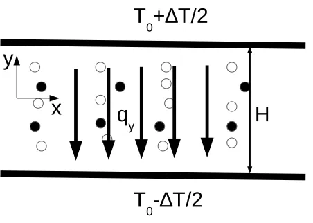
2. Problem statement

Let us consider a binary mixture of monatomic gases, where the mass of a molecule of the first (second) species ism1(m2), and the corresponding number

density is n1 (n2). Without loss of generality, we assume m1 < m2. The

gaseous mixture is confined between two infinitely long parallel plates situated at y0 = ±H/2, see Fig. 1. Both plates are stationary and are kept initially at the same temperature ofT0. Then, instantaneously the temperature of the

both plates changes: the temperature of the down plate decreases toT0−∆T /2

and the temperature of the upper plate increases up toT0+ ∆T /2. We assume

that the temperature difference ∆T is much smaller than the equilibrium gas temperatureT0(∆T T0), so the gaseous mixture deviates only slightly from

its thermodynamic equilibrium and the McCormack model [21] can be applied to simulate the relaxation of the mixture to a new equilibrium state.

The most probable molecular velocity of the mixture is:

v0=

r 2kT0

wherek is the Boltzmann constant and m=C0m1+ (1−C0)m2 is the mean

molecular mass of the mixture. Here,C0is initial equilibrium molar

concentra-tion of the lighter species,

C0=

n01

n01+n02

, (2)

and n0α is the equilibrium number density of speciesα (α= 1,2). The equi-librium number density of the mixture is n0 =n01+n02. The most probable

molecular velocity of speciesαis defined as

v0α= r

2kT0

mα . (3)

We can define the mixture macroscopic velocityu0_y as

u0_y=m1n01u 0

1y+m2n02u02y m1n01+m2n02

. (4)

Here we are interested in the dimensionless heat flux and mixture velocity

qy= q0_y

p0υ0

T0

∆T, uy = u0_y

υ0

T0

∆T, (5)

as well as in the profiles of the deviated temperature, density, and concentration

T= T

0_−T

0

∆T , n=

n0−n0

n0

T0

∆T, C=

C0−C0

C0

T0

∆T. (6)

It is to note that the macroscopic parameters, defined by Eqs. (5), (6) are time (t) and space (y) dependent.

Here the molar concentration of the mixture is defined as

C0= n

0

1

n0

1+n02

. (7)

andn0_α (α= 1,2) is the deviated number density of speciesα,p0 is the

equilib-rium pressure of the mixture,p0=n0kT0. The gas rarefaction is characterized

by the rarefaction parameter which is defined as

δ= H

`, `=

µv0

p0

, (8)

where`is the equivalent mean free path,µ=µ1+µ2is the viscosity of the

mix-ture at the equilibrium temperamix-tureT0and its expression is given in Appendix

Figure 1: Flow geometry

3. Kinetic equation

The Boltzmann kinetic equation is used to simulate the transient heat trans-fer through the gas mixture at arbitrary gas rarefaction. Since only small tem-perature difference between the plates’ surfaces is considered, the Boltzmann equation can be linearized by classical manner as

fα=f_αM(v) [1 +hα∆T /T0], α= 1,2, (9)

wheref_αM is Maxwellian equilibrium distribution function:

fαM(v) =n0α

mα 2πkT0

3/2 exp

−mαv

2

kT0

, (10)

wherevis the molecular velocityαandhαis the perturbation function of species α, which obeys the following two coupled linearized Boltzmann equations [22]

∂hα ∂t0 +vy

∂hα ∂y0 =

2

X

β=1

ˆ

Qαβh, α= 1,2, (11)

where ˆQαβhis the linearized collision term. Here the McCormack model [21] is used for the simulation of the collision term.

It is convenient to introduce, in addition to the already defined by Eqs. (5) and (6) dimensionless variables, the following dimensionless quantities

t= t 0

t0

, y= y

0

H, cα=

v v0α

, Pαyy=− T0

2∆T p0α

P_αyy0 , (12)

scaled by the characteristic time, which is defined as a mean time needed for a molecule to cross the gap between two plates

t0=H/v0. (13)

It is worth to note that this characteristic time is close to the acoustic time, which can be defined here asta =H/

p

γkT0/m(γis the heat capacity ratio).

The ratio between these two times in the case of the monoatomic gases ist0/ta = p

2/γ= 1.095.

For the results analysis, see discussion in Section 5.3, the mean time between the collision is introduced as

tc = ` v0

. (14)

This time can be related to the time-of-flight of molecules in the gap between the plates (or characteristic time)t0 as

tc =t0

δ. (15)

With the introduced above dimensionless variables the linearized Boltzmann equation (11) for speciesαbecomes

∂hα ∂t

r mα

m +cαy

∂hα ∂y = r mα m δA 2 X β=1 ˆ

Lαβh, A=

_C

0

γ1

+1−C0 γ2

. (16)

The expression for the McCormack collisional terms as well as the expressions for the parametersγ1andγ2, the collision frequencies, are provided in Appendix

A.

When the perturbation functionshα(α= 1,2) are known from the solution of Eq. (16), the macroscopic flow characteristics are calculated as follows

nα= 1

π3/2

r _m

mα ˆ

hαexp −c2_αdcα,

uαy= 1 π3/2

r _m

mα ˆ

hαcαyexp −c2α

dcα,

Pαyy = 1 π3/2

ˆ hα

c2_yα−1

3c

2

α

exp −c2_α dcα,

Tα= 1 π3/2

ˆ hα

₂

3c

2

α−1

exp −c2_α dcα,

qαy= 1 π3/2

r _m

mα ˆ

hαcαy

c2_α−5

2

exp −c2_α dcα.

(17)

defined as follows

uy=(C0m1u1y+ (1−C0)m2u2y)/m, T =C0T1+ (1−C0)T2,

qy=C0q1y+ (1−C0)q2y, n=C0n1+ (1−C0)n2,

C=(1−C0)(n1−n2).

(18)

As it was underlined previously all quantities in Eq. (18) depend on time and space variables.

The Maxwell diffuse-specular boundary condition is used to describe the gas-wall interaction:

h+_α(y=1/2)=1−a_αy=1/2h−_α(y=1/2)+ay_α=1/2

ny_α=1/2−3

4+ 1 2c

2

α

,

h+_α(y=−1/2)=1−a_αy=−1/2h−_α(y=−1/2)+ay_α=−1/2

ny_α=−1/2+3 4 −

1 2c

2

α

,

(19)

whereα= 1,2,ayα=±1/2 are the accommodation coefficients of specieαon the upper and down plates, respectively, the superscripts + and −of the pertur-bation function hα in Eq. (19) refer to the outgoing and incoming molecules with respect to the plates’ surfaces, respectively,α= 1,2,nyα=±1/2 is the num-ber density on the plates’ surfaces, which is calculated from non-penetration conditions:

ny_α=1/2=−1

4+ 2 π

ˆ

cαy>0

h−_α(y=1/2)exp −c2_α cαydcα,

ny_α=−1/2= +1 4−

2 π

ˆ

cαy<0

h−_α(y=−1/2)exp −c2_α

cαydcα.

(20)

At the initial timet= 0, the specie perturbation functionhα is zero every-where, so all the deviated macroscopic quantities Eqs. (5), (6) are set equal to 0.

4. Method of solution

The discrete velocity method (DVM) [23] is used to solve the McCormack kinetic equation (16) for each speciesα= 1,2. To reduce computational effort, thecαz variable is eliminated by introducing the reduced functions of hα [24] [25, 26, 27]:

Φα= 1

√

π

r _m

mα ˆ

hαexp −c2αz

dcαz,

Ψα= 1

√

π

r _m

mα ˆ

hαc2_αzexp −c2_αzdcαz.

For the considered one-dimensional heat transfer problem the number of veloci-ties in the molecular velocity space may be still reduced up to one, by eliminating alsocx velocity and so by reducing the computational efforts. However in this study we keep two velocities (cx, cy) formulation, previously used for the steady state Couette and Fourier flows. It is shown below that we obtained the grid convergency in both physical and molecular velocity spaces with the reasonable number of the grid points and, therefore, computational time.

First, the discrete velocity method (DVM) is applied to split the continuum (−∞,∞) molecular velocity spacecx,cyin the governing equation (16) into dis-crete velocity setscxm,cykwherem, k=−Nc, ..,−1,1,2, .., Nc. These velocities cx_m,cy_k are taken to be the roots of the Hermite polynomial of orderNc. Then the set of 2Nc kinetic equations, corresponding to 2Nc values of discrete veloc-ities, is discretized in time and space by finite difference method (FDM). Here Nc is taken to be equal to 20. Grid-independence in molecular velocity space is checked with a finer grid of 50×50 points showing less than 1% difference in all macroscopic profiles.

The spacial derivatives are approximated by the second-order accurate TVD type scheme as in [28]. The number of uniformly distributed points in physical space Ny is equal to 500. The time derivative is approximated by the time-explicit Euler method. The time step, ∆t, is chosen according to the following condition:

∆t=CF L/maxγ1A, γ2A, cNyc/∆y , (22)

whereCF Lis the Courant-Friedrichs-Lewy number which is equal here to 0.5. With the chosen computational grid the last term (cNc

y /∆y) in condition (22) is preponderant, therefore the simulations for both mixtures are carried out with the same time step ∆t= 0.77·10−4_.

For the present simulations the termination condition is defined for the heat flux in following form

min i

q

(l+1)

i −q

(l)

i /

q

(l)

i

≤ε, (23)

wherel is the number of time step,i= 1, Ny, and here ε= 10−7 is used. The termination condition, Eq. (23), is checked for every macroscopic parameter and it is found that the higher order moments like the heat flux, converge more rapidly as the lower one. However we focus our study on the heat flux evolution in time, so the termination condition is applied for the heat flux. The time needed to reach criterion (23) is designated astε.

5. Results and discussion

Two gas mixture of the noble gases with similar mAr_/mN e _{= 1.979 and} disparatemAr_/mHe _{= 9.970 molecular masses are considered. The calculations} were carried out for three values of concentration: C0= 0.1, 0.5 and 0.9 and for

ratio is needed to calculate the collision term in Eq. (11). Here, in the frame of the Hard Sphere molecular model [29] the following data for the diameter ratio dAr/dN e= 1.406 anddAr/dHe= 1.668 were used.

5.1. Transient behaviors of the macroscopic parameters

Initially, att= 0 the gas mixture is in its equilibrium state at temperature T0, then impulsively the temperature of the upper (down) plate increases

(de-creases) to value T0+ ∆T /2 (T0−∆T /2), respectively. The sudden heating

of upper plate and cooling of down plate causes a decrease (increase) in the number density near the upper (down) plate, respectively. This local difference in the mixture number density creates a mass flow of a gas from the upper plate to the down plate and then backwards. Consequently, we observe the number density and macroscopic velocity disturbances propagate in a wave-like manner along the domain; after several time the waves are damped and the macroscopic velocity vanishes.

The transient behaviors of the mixture macroscopic quantities (number den-sity, macroscopic velocity, temperature, and concentration) are represented on Figs. 2 - 5 for two mixtures Ne-Ar and He-Ar, three concentrations of the light species C0 = 0.1, 0.5 and 0.9 and for various values of the rarefaction

parameter ranging from the near free molecular to the slip flow regime. The macroscopic parameters are shown as a function of the dimensionless time, de-fined in Eq. (12). The behaviors of the mixture macroscopic parameters are symmetric (macroscopic velocity and heat flux) and anti-symmetric (number density, temperature and concentration) relatively to the half distance between the plates. Therefore only the data near the hot (upper) plate are plotted, ex-cept for the macroscopic velocity, which is taken at the middle point between the plates.

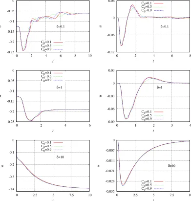
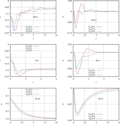
The variations in time of the mixture number density and mixture macro-scopic velocity are shown on Figs. 2 (for Ne-Ar mixture) and 3 (for He-Ar mix-ture), for three values of rarefaction parameter and three concentrations. The number density and velocity behaviors depend strongly on the gas rarefaction. For the higher rarefaction level,δ= 0.1 and 1, the new equilibrium state of the gas mixture is reached through the decaying waves propagating across the gap. The gas mixture moves from the hotter plate toward the colder one and then vise versa to achieve finally the new equilibrium state, where the macroscopic velocity vanishes. Different behaviors of the number density and macroscopic velocity are observed in slip flow regime,δ= 10, the wave structure movement does not appear anymore and only monotone decreasing in the number density is observed with the macroscopic gas movement from the hotter to the colder plate, see Figs. 2 and 3.

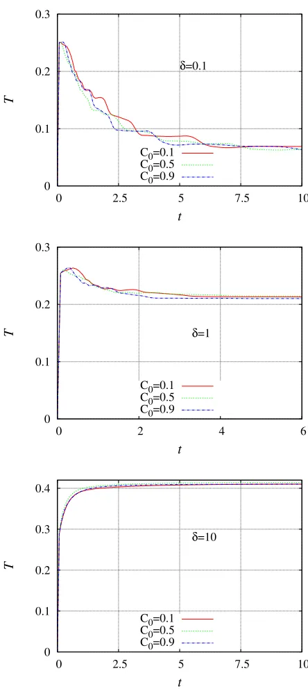
Figure 4 gives information about the time evolution of He-Ar mixture tem-perature. As it was seen for the time evolution of the mixture number density and macroscopic velocity, see Figs. 2 and 3, the temperature time evolution de-pends strongly on the gas rarefaction. After a sudden heating of the upper plate the gas temperature near the wall increases up to its maximum value and then decreases with time up to its equilibrium value. This behavior is observed for δ= 0.1 and 1. The temperature jump between the gas and surface temperatures is clearly seen and it increases with rarefaction parameter decreases. Contrarily, in the slip flow regime, δ = 10, the temperature increases monotonically with time up to its equilibrium value and the temperature jump is much smaller than that in more rarefied conditions. The mixture nature and mixture composition have only slight impact on the transient behavior of the temperature.

The transient behaviors of the light species concentration are shown on Fig. 5 for Ne-Ar and He-Ar mixtures, three initial concentration and various flow regimes. As for the mixture number density, the wave-like structure of the concentration time evolution can be observed with larger number of the waves compared to the number density. The concentration behavior depends strongly on the gas rarefaction. For the higher gas rarefaction, δ = 0.1, the new equi-librium value of the concentration near the hot plate is close to its initial state while with rarefaction decreasing essential rise in the lighter species concentra-tion is observed near the hotter plate. As expected, the time behavior of the concentration depends strongly on the mixture composition and the nature of the mixture.

5.2. Time dependent macroscopic profiles in the gap between the plates

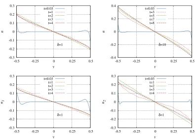
Typical time dependent profiles of the mixture number density, macroscopic velocity and concentration in the gap between the plates are shown in Figs. 6 -8 forC0= 0.5 andδ= 1 and 10, for He-Ar mixtures, respectively. As it is clear

from Figs. 6, the time evolution of the mixture number density profiles show the same trend as in Fig. 3: in the early time the number density decreases (increases) only near the hot (cold) plate, while the rest of the profile remains unchanged. Then, the number density profile converges, but non-monotonically, to the typical mixture number density profile, see Ref. [30]. The species number density evolutions in the gap are shown on Fig. 6 (down line) forδ= 0.1: it is clear that the lighter species He (n1) takes less time, compared to heavier one,

Ar (n2), to converge to its steady state profile.

The wave-like structure can be observed in Figs. 7 and 8 for the time-dependent mixture’ macroscopic velocity profiles and the profiles of the con-centration. The mixture velocity profile tends non-monotonically to zero, see Fig. 7 top line forδ = 1 and 10. Figure 7, down line, demonstrates the time evolution of the macroscopic velocity for each species forC0 = 0.5 andδ = 1.

The concentration profiles, shown on Fig. 8 forδ= 1 and 10, converge also non-monotonically to the typical steady state concentration distribution, where the concentration of the lighter species increases (decreases) near the hot (cold) plate.

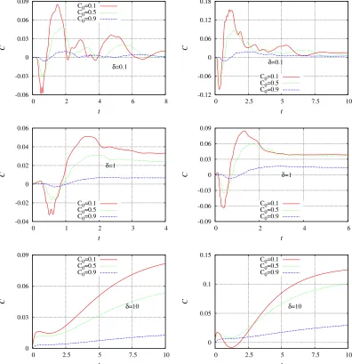
5.3. Heat flux response time

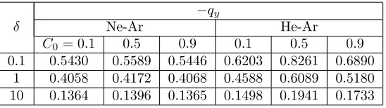
The response time of a media is very important characteristic and it can be useful in the metrology, for example for the development of the fast response sensors. The steady state values of the heat flux between the plates, obtained after the sudden surfaces temperature changes, are provided in Table 1 for two mixtures, three concentrations and three values of the rarefaction parameter. The comparison between the heat flux, provided in Table 1, and similar results from Ref. [10], where the steady-state numerical approach was applied, shows the maximal difference approximately 1%, which is of the order of the reported in Ref. [10] accuracy. From Table 1 it can be seen that for the fixed gas rarefaction, whatever is the flow regime, the heat flux depends slightly on the initial mixture composition for the mixture of the gases with similar molecular masses (Ne-Ar), however for the gas mixture with disparate molecular masses (He-Ar) the mixture composition affects the heat flux.

δ

−qy

Ne-Ar He-Ar

C0= 0.1 0.5 0.9 0.1 0.5 0.9

0.1 0.5430 0.5589 0.5446 0.6203 0.8261 0.6890

1 0.4058 0.4172 0.4068 0.4588 0.6089 0.5180

10 0.1364 0.1396 0.1365 0.1498 0.1941 0.1733

Table 1: The steady state mixture heat fluxqyfor various values of the concentrationC0and the rarefaction parameterδ, for two mixtures: Ne-Ar and He-Ar.

The transient heat flux near the hot surface is plotted on Fig. 9 for two mixtures and for three rarefaction parametersδ= 0.1, 1 and 10 using now the logarithmic scale for time, so the initial transitional time can be better seen. As it is clear from Fig. 9, after the sudden surface temperature changes, the heat flux near the hot surface changes instantaneously from 0 to some value and than keeps this value during certain time. This initial value of the heat flux can be easily found from the simple physical reasoning. During a short time after sudden change of the wall temperature the heat flux is determined only by the distribution function of the molecules reflected from the wall. This time is sufficiently short, so the molecules coming from the opposite wall with different temperature cannot reach yet this wall. We can call here this short time ”early steady state time”, te. This time te depends on the rarefaction level through mean collision time (or time-of-flight of molecules),tc, Eq. (14).

[29]. In the case of diffuse gas-surface interaction it becomes

q0_yα=nαmα 2√π

_2kT

0

mα

3/2_∆T T0

. (24)

Using the dimensionless quantities, Eqs. (2) and (5), the early steady state heat flux of the mixture becomes:

qy= 1

2√π

C0

r_m

m1

+ (1−C0)

r_m

m2

. (25)

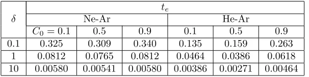
The ”early steady state time”, te, of the mixture heat flux is provided in Table 2 for two mixtures. This time is defined as a time needed for the heat flux to deviate from the analytical value, Eq. (25), in 1%. As can be seen from Fig. 9 and Table 2 this time of quasi constant heat flux decreases withδ increases, decreasing as approximately 1

δ, so with the same tendency as the mean collision time changes with rarefaction level, Eq.(15). This time changes only slightly with the concentration changes for the case of Ne-Ar mixture, with a minimum for the concentrationC0= 0.5. The same tendency with a minimum of timete for the concentration equal to 0.5 is kept for the He-Ar mixture, but only for higher values of the rarefaction parameter.

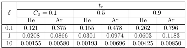
The ”early steady state time”, te, of species heat flux in the case of He-Ar mixture is provided in Table 3. For all considered values of concentration and the rarefaction level the timete for the lighter species (He) is alway lower than that of the larger one (Ar) with the ratiotAr_e /tHe_e of the order of 2-4.

During the early steady time the particles from the cold wall have not reached yet the hot wall and the solution is determined only by the molecules in the vicinity of the hot wall. These results are in agreement with the analytical solution obtained in [12] for a single gas and with the numerical results provided in [20] in the case of the gas mixture between two coaxial cylinders. This particularity of the heat flux evolution in time needs to be take into account when one estimates the response time of the various sensors.

δ

te

Ne-Ar He-Ar

C0= 0.1 0.5 0.9 0.1 0.5 0.9

0.1 0.325 0.309 0.340 0.135 0.159 0.263

1 0.0812 0.0765 0.0812 0.0464 0.0386 0.0618

10 0.00580 0.00541 0.00580 0.00386 0.00271 0.00464

Table 2: The ”early steady state time”,te, of the mixture heat flux for Ne-Ar and He-Ar mixtures, for different initial concentrationC0and rarefaction parameterδ.

δ

te

C0= 0.1 0.5 0.9

He Ar He Ar He Ar

0.1 0.121 0.375 0.155 0.478 0.262 0.796

1 0.0208 0.0866 0.0301 0.0974 0.0603 0.1183

10 0.00155 0.00580 0.00193 0.00696 0.00425 0.00850

Table 3: The ”early steady state time”,te, for He-Ar mixture, for different initial concentration

C0and rarefaction parameterδ.

masses (He−Ar), see Fig. 9 (right column), the relaxation speed of heat flux is affected by the species concentration. The heat flux behavior depends strongly on the rarefaction level: the heat flux decreases with time for higher level of gas rarefaction (δ = 0.1 and 1) and increases to its new equilibrium value for δ= 10.

Figure 10 shows the heat flux profiles for Ne-Ar mixture withC0 = 0.5 as

a function of the position in the gap between the plates and for various time moments for two values of the rarefaction parameterδ = 1 and 10. It can be seen from Fig. 10 that the transient behavior of the total heat flux depends on the distance to the plates and on the rarefaction level. Forδ = 1 the heat flux decreases with time in the whole gap. However, forδ= 10, this behavior changes in the vicinity of the plates: the heat flux decreases up to a value and then increases to its new equilibrium state.

The time needed to reach the convergence criterion (23), tε, was obtained for different values of initial concentration C0 and rarefaction parameter. The

values of tε are presented in Table 4. It is interesting to note that for a fixed initial concentrationC0this timetεhas a minimum value in the transitional flow regime whatever the concentration or the mixture composition. For the fixed level of the gas rarefaction the minimumtε is reached for C0 = 0.5 whatever

the mixture composition.

δ

tε

Ne-Ar He-Ar

C0= 0.1 0.5 0.9 0.1 0.5 0.9

0.1 13.37 10.66 12.90 9.66 9.27 10.12

1 4.40 4.25 4.32 4.40 4.32 4.40

10 9.98 9.60 9.60 9.71 8.82 7.46

Table 4: Timetε needed to satisfy criterion (23) for different initial concentrationC0 and rarefaction parameterδ.

this steady state time decreases with increase of light component fraction. For higher level of gas rarefaction (δ= 0.1 and 1) the time to reach the steady state has a maximum forC0= 0.5. For the Ne-Ar mixture this steady state time for

C0 = 0.5 is 3.8−4.4% higher compared to the concentration C0 = 0.1. This

difference in the steady state time increases for He-Ar mixture up to 20% for δ= 0.1. At the fixed value of concentration parameterC0 steady state timets

δ

ts

Ne-Ar He-Ar

C0= 0.1 0.5 0.9 0.1 0.5 0.9

0.1 1.78 1.85 1.70 1.78 2.24 1.31

1 1.70 1.78 1.70 1.78 2.08 1.23

10 7.47 7.06 6.57 7.00 5.14 3.81

Table 5: The steady state time,ts, a time needed to obtain the value of the heat flux in the gap, which is different in 1% from its steady state value for different values of initial concentrationC0 and rarefaction parameterδ.

takes the minimum value in transitional flow regime (δ= 1). This behavior is similar to the results of Ref. [20], where the minimum of the steady state time was found in the transitional flow regime when the heat transfer through the gas mixture between two coaxial cylinders is analyzed. In the slip flow regime the steady state time decreases with increasing of the concentration of the lighter species and it is lower for the He-Ar mixture.

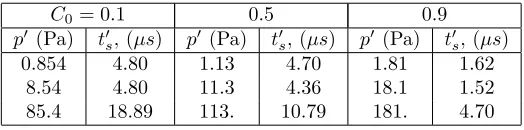
For the practical application it is interesting to have an idea on the order of magnitude of the steady state time at a given pressure. From the data pro-vided in Table 5 we can estimate this time. Let us consider a small distance between the plates of 1mmand the reference temperatureT0equal to 300K. The

mixture viscosity can be evaluated, for example, using the Wilke formula [31]. Then, from the given rarefaction parameter a pressure can be calculated and the corresponding steady state time. These values for He-Ar mixture and three concentrations are provided in Table 6. For a fixed equilibrium concentration of

C0= 0.1 0.5 0.9

p0 (Pa) t0_s, (µs) p0 (Pa) t0_s, (µs) p0 (Pa) t0_s, (µs)

0.854 4.80 1.13 4.70 1.81 1.62

8.54 4.80 11.3 4.36 18.1 1.52

85.4 18.89 113. 10.79 181. 4.70

Table 6: The dimensional steady state time,t0s, for He-Ar mixture.

the lighter speciesC0 significantly more time is needed for the heat flux

6. Conclusion

The transient heat transfer due to the sudden change of the walls’ temper-atures through a binary gas mixture was simulated on the basis of numerical solution of kinetic model equation with McCormack collision integral in a wide range of rarefaction parameter and species concentrations. The cases of small and large species mass ratio were considered. The time needed for the heat flux to reach its new equilibrium steady state condition, steady state time, was es-tablished for both mixtures, three concentrations and different rarefaction level. It was found that in the near free molecular and transitional flow regimes this steady state time has a maximum for the concentration equal to 0.5, whatever is the mixture composition, while in the slip flow regime the steady state time de-creases with increasing of the lighter species concentration. For the fixed value of the concentration the time has a minimum in the transitional flow regime. The particular behavior is observed just after the sudden temperature change: the heat flux keeps a constant value during 0.03 - 0.3 characteristic times depending on the gas rarefaction and then starts to evolve to new equilibrium state. The time evolution of macroscopic quantities, number density, macroscopic velocity, temperature and concentration, were obtained for both mixtures and in large rarefaction parameter range.

Acknowledgement

M. T. Ho and I. Graur thank the Labex MEC project (ANR-10-LABX-0092) and the A*MIDEX project (ANR-11-IDEX-0001-02), funded by the ”Investisse-ments d’Avenir” French Government program managed by the French National Research Agency (ANR), for their support. A. Polikarpov thanks the Russian Science Foundation (project No. 1419-01755) for its financial support.

[1] D R Willis. Heat transfer in a rarefied gas between parallel plates at large temperature ratios. In J A Lauermann, editor, Rarefied Gas Dynamics, volume 1, pages 209–225. Academic Press, New York, 1963.

[2] P Bassanini, C Cercignani, and C D Pagani. Comparison of kinetic theory analysis of linearized heat transfer between parallel plates. Int. J. Heat Mass Transfer, 10:447–460, 1967.

[3] P Bassanini, C Cercignani, and C D Pagani. Influence of the accommo-dation coefficient on the heat transfer in a rarefied gas. Int. J. Heat Mass Transfer, V.11, pp. 1359-1368, 1968.

[4] J R Thomas, T S Chang, and Siewert C E. Heat transfer between parallel plates with arbitrary surface accommodation. Physics of Fluids, 16(12), 1973.

the Boltzmann equation for hard sphere molecules. Physics of Fluids A, 1(12):2042–2049, 1989.

[6] C E Siewert. Viscous-slip, thermal-slip and temperature-jump coefficients as defined by the linearized Boltzmann equation and the Cercignani-Lampis boundary condition. Phys. Fluids, 15(6):1696–1701, 2003.

[7] I A Graur and A Polikarpov. Comparison of different kinetic models for the heat transfer problem. Heat and Mass Transfer, 46:237–244, 2009.

[8] S Kosuge, K Aoki, and S Takata. Heat transfer in a gas mixture between two parallel plates: finite-difference analysis of the Boltzmann equation. In T J Bartel and M A Gallis, editors, Rarefied Gas Dynamics, volume 585, pages 289–296, Melvile, 2001. 22nd Int. Symp., AIP Conference Proc.

[9] R D M Garcia and C E Siewert. The McCormack model for gas mixtures: Heat transfer in a plane channel. Phys. Fluids, 16(9):3393–3402, 2004.

[10] F Sharipov, L M G Cumin, and D Kalempa. Heat flux through a binary gaseous mixture over the whole range of the knudsen number. Physica A, 378:183–193, 2007.

[11] Sone Y. Effect of sudden change of wall temperature in a rarefied gas. J. Phys. Soc. Jpn., 20(2):222–229, 1965.

[12] M Perlmutter. Analysis of transient heat transfer through a collisionless gas enclosed between parallel plates. ASME Paper 67-HT-53, 1967.

[13] D C Wadsworth, D A Erwin, and E Ph Muntz. Transient motion of a con-fined rarefied gas due to wall heating or cooling. Journal of Fluid Mechanics, 248(1):219, April 1993.

[14] A Manela and N. G. Hadjiconstantinou. On the motion induced in a gas confined in a small-scale gap due to instantaneous boundary heating. J. Fluid Mechanics, 593(11):453–462, 2007.

[15] A Manela and N. G. Hadjiconstantinou. Gas motion induced by unsteady boundary heating in a small-scale slab. Phys. Fluids, 20(11):117104(11 pages), 2008.

[16] T. Doi. The mccormack model for gas mixtures: Heat transfer in a plane channel. Journal of Heat Transfer, 133(9):022404(9 pages), 2011.

[17] O Buchina, M Vargas, S Stefanov, and D Valougeorgis. Transient micro heat transfer in a gas confined between parallel plates due to a sudden increase of the wall temperature. In 3rd Micro and Nano Flows Conference (MNF2011), Thesaloniki, Greece, August 22-24, 2011.

[19] D Kalempa and F Sharipov. Numerical modelling of thermoacoustic waves in a rarefied gas confined between coaxial cylinders. Vacuum, 109:326–332, 2014.

[20] M Vargas, S Stefanov, and V Roussinov. Transient heat transfer flow through a binary gaseous mixture confined between coaxial cylinders. International Journal of Heat and Mass Transfer, 59:302–315, 2013.

[21] F J McCormack. Construction of linearized kinetic models for gaseous mixture and molecular gases. Phys. Fluids, 16:2095–2105, 1973.

[22] J H Ferziger and H G Kaper. Mathematical Theory of Transport Processes in Gases. North-Holland Publishing Company, Amsterdam, 1972.

[23] F Sharipov, L M G Cumin, and D Kalempa. Plane Couette flow of binary gaseous mixture in the whole range of the Knudsen number. Eur. J. Mech. B/Fluids, 23:899–906, 2004.

[24] S Naris, D Valougeorgis, F Sharipov, and D Kalempa. Discrete ve-locity modelling of gaseous mixture flows in mems. Superlattices and Microstructures, 35(3-6):629 – 643, 2004.

[25] C K Chu. Kinetic-theoretic description of the formation of a shock wave. Phys. of Fluids, 12(8):12–22, 1965.

[26] A B Huang and Hartley D L. Kinetic theory of the sharp leading edge problem in supersonic flow. Phys. of Fluids, 96(12):96–108, 1969.

[27] P Andries and B Perthame. The es-bgk model equation with correct prandtl number. In Rarefied Gas Dynamics, AIP Conference Proceedings, volume 585, pages 30–36, 2001.

[28] A.Ph. Polikarpov and I. Graur. Unsteady rarefied gas flow through a slit. Vacuum, 101:79 – 85, 2014.

[29] G A Bird. Molecular Gas Dynamics and the Direct Simulation of Gas Flows. Oxford Science Publications, Oxford University Press Inc., New York, 1994.

[30] M T Ho, L Wu, I Graur, Y Zhang, and Reese J M. Comparative study of the boltzmann and mccormack equations for couette and fourier flows of binary gaseous mixtures. Int. J. Heat Mass Transfer, 96:29–41, 2016.

[31] C R Wilke. A viscosity equation for gas mixture. Journal Chem. Phys., 18(4):517–522, 1950.

[32] E M Shakhov. Generalization of the Krook kinetic relaxation equation. Fluid Dyn., 3(5):95–96, 1968.

-0.25 -0.2 -0.15 -0.1 -0.05 0

0 2 4 6 8 10

n

t δ=0.1

C0=0.1 C0=0.5 C0=0.9

-0.12 -0.06 0 0.06

0 2 4 6 8

u

t δ=0.1 C₀=0.1

C₀=0.5 C₀=0.9

-0.25 -0.2 -0.15 -0.1 -0.05 0

0 2 4 6

n

t δ=1 C₀=0.1 C₀=0.5 C₀=0.9

-0.09 -0.06 -0.03 0 0.03

0 1 2 3 4

u

t δ=1

C₀=0.1 C₀=0.5 C₀=0.9

-0.4 -0.3 -0.2 -0.1 0

0 2.5 5 7.5 10

n

t δ=10 C₀=0.1 C₀=0.5 C0=0.9

-0.035 -0.028 -0.021 -0.014 -0.007 0

0 2.5 5 7.5 10

u

t

δ=10

C₀=0.1 C₀=0.5 C₀=0.9

-0.25 -0.2 -0.15 -0.1 -0.05 0

0 2.5 5 7.5 10

n

t δ=0.1

C0=0.1 C0=0.5 C0=0.9

-0.12 -0.06 0 0.06

0 2.5 5 7.5 10

u

t δ=0.1

C0=0.1

C0=0.5

C0=0.9

-0.25 -0.2 -0.15 -0.1 -0.05 0

0 2 4 6

n

t δ=1 C₀=0.1 C₀=0.5 C₀=0.9

-0.09 -0.06 -0.03 0 0.03

0 2 4 6

u

t δ=1

C₀=0.1 C₀=0.5 C₀=0.9

-0.4 -0.3 -0.2 -0.1 0

0 2.5 5 7.5 10

n

t δ=10 C₀=0.1 C₀=0.5 C0=0.9

-0.04 -0.02 0

0 2.5 5 7.5 10

u

t δ=10

C₀=0.1 C₀=0.5 C₀=0.9

0 0.1 0.2 0.3

0 2.5 5 7.5 10

T

t

δ=0.1

C₀=0.1 C₀=0.5 C₀=0.9

0 0.1 0.2 0.3

0 2 4 6

T

t

δ=1

C₀=0.1

C₀=0.5

C₀=0.9

0 0.1 0.2 0.3 0.4

0 2.5 5 7.5 10

T

t

δ=10

C₀=0.1

C₀=0.5

C₀=0.9

-0.06 -0.03 0 0.03 0.06 0.09

0 2 4 6 8

C

t δ=0.1 C₀=0.1

C₀=0.5 C₀=0.9

-0.12 -0.06 0 0.06 0.12 0.18

0 2.5 5 7.5 10

C

t δ=0.1

C0=0.1 C0=0.5 C0=0.9

-0.04 -0.02 0 0.02 0.04 0.06

0 1 2 3 4

C

t δ=1

C₀=0.1 C₀=0.5 C₀=0.9

-0.09 -0.06 -0.03 0 0.03 0.06 0.09

0 2 4 6

C

t δ=1

C₀=0.1 C₀=0.5 C₀=0.9

0 0.03 0.06 0.09

0 2.5 5 7.5 10

C

t

δ=10 C₀=0.1

C₀=0.5 C0=0.9

0 0.05 0.1 0.15

0 2.5 5 7.5 10

C

t δ=10 C₀=0.1 C₀=0.5 C0=0.9

-0.3 -0.2 -0.1 0 0.1 0.2 0.3

-0.5 -0.25 0 0.25 0.5

n

y δ=1 t=0.03

t=1 t=2 t=3 t=4

-0.4 -0.2 0 0.2 0.4

-0.5 -0.25 0 0.25 0.5

n

y δ=10 t=0.03

t=3 t=5 t=7 t=8

-0.3 -0.2 -0.1 0 0.1 0.2 0.3

-0.5 -0.25 0 0.25 0.5

n1

y δ=1 t=0.03

t=1 t=2 t=3 t=4

-0.3 -0.2 -0.1 0 0.1 0.2 0.3

-0.5 -0.25 0 0.25 0.5

n2

y δ=1 t=0.03

t=1 t=2 t=3 t=4

Figure 6: Top line: profiles of mixture number density between the plates forHe−Armixture,

-0.06 -0.045 -0.03 -0.015 0 0.015

-0.5 -0.25 0 0.25 0.5

u y δ=1 t=0.03 t=1 t=2 t=3 t=4 -0.04 -0.02 0

-0.5 -0.25 0 0.25 0.5

u y δ=10 t=0.03 t=3 t=5 t=7 t=8 -0.12 -0.1 -0.08 -0.06 -0.04 -0.02 0 0.02

-0.5 -0.25 0 0.25 0.5

u1 y δ=1 t=0.03 t=1 t=2 t=3 t=4 -0.06 -0.045 -0.03 -0.015 0 0.015

-0.5 -0.25 0 0.25 0.5

u2 y δ=1 t=0.03 t=1 t=2 t=3 t=4

Figure 7: Top line: profiles of mixture macroscopic velocity between the plates forHe−Ar

mixture,C0= 0.5;δ= 1 and 10; down line: the species macroscopic velocity evolution, He (u1) and Ar (u2) forδ= 1 andC0= 0.5.

-0.06 -0.04 -0.02 0 0.02 0.04 0.06

-0.5 -0.25 0 0.25 0.5

C y δ=1 t=0.03 t=1 t=2 t=3 t=4 -0.1 -0.05 0 0.05 0.1

-0.5 -0.25 0 0.25 0.5

C y δ=10 t=0.03 t=3 t=5 t=7 t=8

-0.6 -0.4 -0.2

0.01 0.1 1 10 100

qy

t δ=0.1

C₀=0.1 C₀=0.5 C₀=0.9

-0.9 -0.6 -0.3

0.0001 0.001 0.01 0.1 1 10 100

qy

t δ=0.1

C₀=0.1

C0=0.5

C0=0.9

-0.45 -0.3 -0.15

0.0001 0.001 0.01 0.1 1 10 100 qy

t δ=1 C₀=0.1 C₀=0.5 C₀=0.9

-0.65 -0.5 -0.35 -0.2

0.0001 0.001 0.01 0.1 1 10 100

qy

t

δ=1

C₀=0.1

C₀=0.5

C₀=0.9

-0.3 -0.2 -0.1 0

0.0001 0.001 0.01 0.1 1 10 100

qy

t δ=10

C₀=0.1

C₀=0.5

C₀=0.9

-0.45 -0.3 -0.15 0

0.0001 0.001 0.01 0.1 1 10 100 qy

t

δ=10 C₀=0.1

C₀=0.5 C₀=0.9

Figure 9: Time evolution of normal heat flux near the hot plate for two gas mixturesN e−Ar

-0.45 -0.3 -0.15 0

-0.5 -0.25 0 0.25 0.5

qy y δ=1 t=0.03 t=1 t=2 t=3 t=4 -0.3 -0.2 -0.1 0

-0.5 -0.25 0 0.25 0.5

qy y δ=10 t=0.03 t=3 t=5 t=7 t=8

Figure 10: Profiles of normal heat flux between the plates forN e−Armixture andC0= 0.5

Appendix A. The McCormack collision term

The dimensionless collision term of the McCormack model [21] in eq. (16) has the following form:

ˆ

Lαβh=−γαβhα+γαβnα

+ 2 r

mα m

"

γαβuαy−υ_αβ(1)(uαy−uβy)−υ

(2)

αβ 2

qαy−mα

mβqβy

#

cαy

+

γαβTα−2mαβ mβ

(Tα−Tβ)υ(1)_αβ c2_α−3

2

+2hγαβ−υ_αβ(3)Pαyy+υ_αβ(4)Pβyyi

c2_αy−1

2c 2 αx− 1 2c 2 αz +4 5 r mα m γαβ−υ

(5)

αβ

qαy+υ

(6)

αβ

r_m

β mαqβy−

5 4υ

(2)

αβ(uαy−uβy)

cαy

c2_α−5

2

,

whereα, β= 1,2, andυ_αβ(i) are defined as following

υ_αβ(1)= 16 3

mαβ mα

nβΩ11_αβ,

υ_αβ(2)= 64 15 _mαβ mα 2 nβ

Ω12_αβ−5

2Ω

22

αβ

,

υ_αβ(3)= 16 5

m2_αβ

mαmβnβ 10 3 Ω 11 αβ+ mβ mαΩ 22 αβ ,

υ_αβ(4)= 16 5

m2

αβ mαmβnβ

₁₀

3 Ω

11

αβ−Ω

22

αβ

,

υ_αβ(5)= 64 15 mαβ mα 3 mα mβnβ Ω22αβ+

15 4 mα mβ + 25 8 mβ mα Ω11αβ−

1 2

mβ

mα 5Ω

12

αβ−Ω13αβ

,

υ_αβ(6)= 64 15

_mαβ

mα

3_mα

mβ 3/2

nβ

−Ω22_αβ+55 8 Ω 11 αβ− 5 2Ω 12 αβ+ 1 2Ω 13 αβ , (A.2) where

mαβ=

mαmβ

mα+mβ (A.3)

is the reduced mass of the binary mixture. Note that Ω(_αβi,j) in Eq. (A.2) rep-resents the omega integral [22], which for the case of the HS model is defined as [22]

Ω(_αβi,j)= (j+ 1)! 8

"

1−1 + (−1)

i

2(i+ 1) #

_πkT

2mαβ 1/2

(dα+dβ)2. (A.4)

Finally, the parameters γαβ are proportional to the collision frequency be-tween speciesαandβ and appear in the collision term (A.1) only in the combi-nationsγ1=γ11+γ12andγ2=γ21+γ22, so one has only to defineγ1 andγ2.

The collision frequencies and the viscosity can be related in the same manner as in the Shakhov kinetic equation [32, 33, 23]:

γα= p0α

µα, (A.5)

where p0α = n0αkT0 is the equilibrium partial pressure and µα is the partial viscosity given as

µα=p0α

Sβ+υ

(4)

αβ

SαSβ−υ(4)_αβυ_βα(4)

, Sα=υ(3)_αα−υ(4)_αα+υ_αβ(3), and β 6=α. (A.6)