City, University of London Institutional Repository
Citation
:
Pantelous, Athanasios (2013). Solutions Properties and Techniques for Implicit Systems. (Unpublished Doctoral thesis, City University London)This is the unspecified version of the paper.
This version of the publication may differ from the final published
version.
Permanent repository link:
http://openaccess.city.ac.uk/3513/Link to published version
:
Copyright and reuse:
City Research Online aims to make research
outputs of City, University of London available to a wider audience.
Copyright and Moral Rights remain with the author(s) and/or copyright
holders. URLs from City Research Online may be freely distributed and
linked to.
City Research Online: http://openaccess.city.ac.uk/ [email protected]
“Solutions Properties and Techniques for
Thesis submitted for the award of the degree of
CONTROL ENGINEERING RESEARCH CENTER
SCHOOL OF ENGINEERING
i
Solutions Properties and Techniques for
Implicit Systems”
by
Athanasios A Pantelous
Thesis submitted for the award of the degree of
Doctor of Philosophy
in
Systems and Control Theory
CONTROL ENGINEERING RESEARCH CENTER
SCHOOL OF ENGINEERING AND MATHEMATICAL SCIENCES
CITY UNIVERSITY
LONDON EC1V 0HB
OCTOBER 2013
Solutions Properties and Techniques for
Thesis submitted for the award of the degree of
CONTROL ENGINEERING RESEARCH CENTER
ii
“Solutions Properties and Techniques for
iii
v
Declaration
The University Librarian of the City University may allow this thesis to be copied in
whole or in part without any reference to the author. This permission covers only single
vii
Table of Contents
Frequently used Notations ... xi
List of Figures ... xvi
Acknowledgments ... xviii
CHAPTER 1: Introduction – Contribution ... 21
CHAPTER 2: Approximating Distributional Behaviour of Linear Systems Using Gaussian Function and its Derivatives ... 29
2.1 Introduction ... 29
2.2 Problem Definition ... 32
2.3 Approximation of Dirac Delta Function ... 35
2.3.1 Infinite Time-Support Domain ... 36
2.3.2 Finite Time-Support Domain ... 38
2.3.3 Why a Sum of Dirac Delta Functions? ... 39
2.4 Design of Approximate Input Signal ... 41
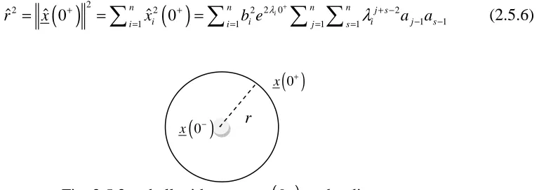
2.5 Distance Problems ... 50
2.5.1. Distance from the origin in state-space ... 50
2.5.2 Maximum distance from the origin with constrained input ... 51
2.6 Conclusions – Further Research ...58
viii
3.1 Introduction ... 61
3.2 The Generalized Inverses of the Vandermonde Matrix ... 68
3.3 The Generalized Inverse of a Special Matrix ... 84
3.4 Conclusions – Further Research ... 92
CHAPTER 4: Generalized Regular Differential Systems with Distributed Delay 93 4.1 Introduction ... 93
4.2 Mathematical Background from Matrix Pencil Theory ... 95
4.3 Delay Differential Equations and Renewal Equations ... 99
4.4 Systems of Generalized Linear Differential Equations with Distributed Delay ... 102
4.5 A Numerical Application ... 109
4.6 Conclusions – Further Research ... 111
CHAPTER 5: On Linear Generalized Neutral Differential Delay Systems ... 113
5.1 Introduction ... 113
5.2 Matrix Pencil Theory Background ... 115
5.3 Systems of Linear Generalized Neutral Differential Delay Equations ... 119
5.4 An Illustrative Example ... 129
5.5 Conclusions – Further Research ... 131
CHAPTER 6: On Generalized Regular Stochastic Differential Delay Systems with Time Invariant Coefficients ... 133
ix
6.2 Preliminaries on Linear Stochastic Delay Differential Equations ... 135
6.2.1 Differential – Algebraic Systems (DASs) ... 135
6.2.2 Linear Delay Differential Systems (DDSs) ... 136
6.3 Generalized Stochastic (Random) Processes ... 139
6.4 Systems of Generalized Linear Regular Stochastic Delay Differential Equations 141 6.5 The Main Results with Respect to Certain Type of Noises ... 148
6.5.1 Brownian Motion (or White Noise) ... 148
6.5.2 Fractional Brownian Motion (or Fractional White Noise) ... 149
6.6 Conclusion - Further Research ... 152
CHAPTER 7: Conclusions - Further Research ... 155
References ... 163
xi
Frequently Used Notations
∞: infinity
ε
: absolute errorΩ: sample space
ω: event, outcome
a∈A: a element of setA
( )
A
I ⋅ : indicator function of event A
P: probability measure
A: σ −algebra
(
Ω,F P,)
: probability spacen
ℝ : n-dimensional Euclidean space
+
ℝ : positive real line
F: Field
(
n m× ;)
M F : algebra of n m× -matrices with elements over F
1
n′−
D : space of Dirac distribution having derivatives up to an order n−1
D : space of infinitely differentiable complex-valued functions on F
( )
B D : Borel σ-field
( )
C∞ ⋅ : set of smooth functions
( )
2
L ⋅ : space of quadratically integrable functions
a.s.: almost surely
[ ]
a b, : closed interval from a to b( )
a b, : open interval from a to bLTI : Linear Time Invariant
( )
x t : state vector parameter
( )
u t : input vector parameter
( )
xii
a : input signal
2
⋅ : Euclidean distance
( )
t
δ
: Dirac function( )k
( )
tδ
: kth derivative of the Diracδ
-function( )
a t
δ
: nascent delta function( )
tϕ
: test function1 ,
ij i j n
A a
≤ ≤
= : constant matrix in ℝn n×
{}
diag ⋅ : diagonal matrix
det A: determinant of matrix A
J: Jordan canonical form of matrix A.
O: zero matrix
(
)
, 1, 2,...,
m n n m
V ≡V
λ λ
λ
: Vandermonde matrix, which is defined in terms of scalars1, 2,..., m
λ λ λ ∈ℝ (where m ≠n)
1
A− : inverse matrix A
†
A : Moore-Penrose inverse of a matrix A D
A : Drazin inverse of square matrix A
{1,2,3}
A : {1, 2, 3}- generalized inverse of matrix A.
q
H : nilpotent matrix
*
q : the annihilation index of Hq
( )
Ind A : the smallest non-negative integer such as rank A
(
Ind A( ))
=rank A(
Ind A( )+1)
[ ]
( )
n
C ⋮ : the n-order compound matrix of
[ ]
⋮( )
Re
λ
: real part of a complex number λ( )
Im
λ
: imaginary part of a complex number λ*: conjugate transpose index of the relevant matrix
xiii
⋅
∐
: order left multiplication of matricesLU: “Lower Upper” factorization
1,2, ,
max
j z
z d
ρ
µ
= =
… : index of annihilation for the eigenvalue µz.
n
ɶ: set
{
1, 2,...,n}
ODE: ordinary differential equation
NBV: normalized bounded variation function
GDDS: generalized differential delay system
DDDS: differential systems with distributed delay
DDE: delay differential equation
DAS: differential-algebraic system
SVD: singular value decomposition
e.d.: elementary divisors
z.e.d.: zero elementary divisors
nz. f.e.d.: nonzero finite elementary divisors
i.e.d.: infinite elementary divisors
c.m.i.: column minimal indices
r.m.i.: row minimal indices
[ ]
s s,ˆF : ring of polynomials in s and sˆ 1/= s with coefficients on F
sF G− : the pencil
(
F G,)
g
e :
(
I In, n)
identity element of the group( )
g,∗ on the set of Lrn n,s
E : a strict equivalence relation
,
r n n
L : the set on n×n regular pencils
( )
z∆ : the characteristic matrix defined by
( )
o
o t
zt t
zI A e d t
τ
µ
+−
−
∫
.:
µ
NBV function[
t to, o+ →τ
]
ℂn n×sBm: standard Brownian motion
xiv
( )
0,1∈
H : Hurst parameter
( )
WH t : Representation of fBm of Hurst parameter
( )
aΓ : Gamma function
X
F : distribution function of random variable X
( )
1 2/ 22 x
x e
π
φ = − : the Gaussian probability density function
( )
1 2/ 2 2x
x e dx
π
∞ ∞
− −
Φ =
∫
: the Gaussian cumulative distribution function( )
( ),
K t
x dx
σ
φ
−∞∫
: the cumulative distribution function (cdf) of a random variable~ (0,1)
X N evaluated at the upper limit of the integral K t
( )
,σ
, denoting the probability that X ≤K t( )
,σ
.( )
,K t
σ
: t/σ... dt
∫
: (Lebesgue, Riemann) integral... dWt
∫
: Ito integral( )
...
L
dz
γ
∫
: so-called principal value integral limi i
dz
γ ω
ω γ ω
+
→∞ −
∫
…
( )
W t : Wiener process at time t
ΙΓH: a transformation which transforms the white noise (the derivative of
sBm) to fractional noise (the derivative of fBm)
( ) ( )
,o T t
s dW s
ξ ϕ
=∫
ϕ
:generalized stochastic (random) process
( ) ( )
,S
S S
σδ ϕ
=∫
ϕ ξ σ ξ δ
: the linear continuous functional σδS on the space D of infinitely differentiable complex-valued functions on F with compactxv
List of Figures
xvii
Acknowledgements
Acknowledgements
Acknowledgements
Acknowledgements
These few lines seem painfully inadequate for me to thank all those who have helped me and supported me through all the years of my research.
I hope to continue supporting me for many more years.
Definitely, I owe an immeasurable debt to my supervisor Prof. Nicos Karcanias, who has guided me through that time. His valuable comments and constructive criti-cism, his continuous support and understanding, became my cornerstone the last six years.
I am really very grateful to my external and internal examiner Prof. Gaynor Taylor and Prof. Martin Newby respectively, who have afforded me considerable assistance in en-hancing both the quality of the findings and the clarity of my PhD thesis presentation.
Words cannot express my gratitude to my beloved family who gave me the op-portunity to pursue my dreams in the UK. Your unconditional love and support is my safety blanket.
Thanks a lot!
18
19
Chapter 1
Chapter 1
Chapter 1
Chapter 1
Introduction – Contribution
In economic theory, input-output analysis has been developed for the description of
the production of a multi-sector economy. An input-output model is a quantitative
eco-nomic technique that represents the interdependencies between different branches of a
national economy or different regional economies. In the region of input-output
eco-nomics, many models were established to describe the real economics (see for example,
Leontief (1966) and R. O'Connor, E.W. Henry (1975)).
The economic traditional Leontief dynamic input-output model is described by
[
1]
k k k k k
x =Ax +L x+ −x +g ,
where the vector xk =x1,k x2,k ⋯ xn k, T is the total output vector and x is the i k,
total output from sector 1 i≤ ≤n. The vector g is the final net product and k g de-i k, notes the final net product of sector 1 i≤ ≤n. The matrix A=aij,1≤i j, ≤n, is the
direct consumption coefficient matrix (also called the Leontief intput-output matrix) and
,
ij
L= l 1≤i j, ≤n, is the capital coefficient matrix. Initially, this model has been
stud-ied in discrete-time where the matrices A and L have been assumed to be constant over
time, i.e. that market and technology do not change under the considered time period.
The discrete-time version of this input-output model has been used widely because of
the nature of the problem (see for example Luenberger and Arbel (1977), Szyld (1985)
and references therein). However, as it is true, the production of a nation (or a factory)
in real economic terms is in fact continuous. Thus, an analogous continuous in time
20
( )
( )
( ) ( )
x t = Ax t +Lx tɺ +g t , t>0,
has been also proposed and studied in the literature of economic modelling (see
Fleissner (1990), Jodar and Merello (2010), Zhao and Jiang (2009) and references
there-in). In this input-output model, the capital coefficient matrix L is not always invertible,
since the product of some sectors can not be treated as a capital product or/and utilized
by others (for example, agriculture, service sectors also do not produce durable goods
etc.). In fact, the element l of matrix ij Lrepresents the amount of stock of commodity i, as a capital good, that sector j must have on hand for each unit of production. Since not
every sector produces significant capital goods, it is common for some rows of the
ma-trix L to contain only zero elements. System above, which can be formally written as
( )
( ) ( )
Lx tɺ =Mx t + f t , t>0,
where M = −I A, f t
( )
= −g t( )
and L is a non-invertible constant matrix, is a linear time invariant (LTI) singular system and it is often called degenerate (or of descriptortype). It is useful here to emphasize that the parameter f t
( )
, t≥0 can be considered either as just a (regular or irregular) disturbance or as the Leontief dynamic input-outputmodel's control vector, as long as the quantity of the final net product can be affected by
various ways.
However, in Engineering now, very recently, in the very interesting paper by
Kar-canias (2008), we can see that the always challenging problem of integrated engineering
design, which is strongly linked to systems and control theory (and their applications),
is revealed as a typical structure evolution process. Such processes emerge in many
ap-plication domains and in the engineering context in problems such as integrated system
design, integrated operations, re-engineering, lifecycle design issues, networks etc.
Thus, it has been shown that the formation of the system, which is finally used for
con-trol design, evolves during the earlier design stages. The process synthesis and the
over-all instrumentation are also critical stages of the evolutionary process that shapes the
21
revealing the control theory context of the evolutionary mechanism in overall system
design.
Familiarizing with the proposed results by Karcanias (2008), we can also claim that
the characteristics and the nature of the process synthesis and the global instrumentation
depend on the type of available models. Thus, there are models where some of the
in-ternal variables are classified into potential inputs, outputs, inin-ternal variables and
re-ferred to as oriented models, or models where no classification has been made of the
internal variables these are called implicit models. All such models may be used for
se-lection of effective sets of inputs and outputs, they are referred to as progenitor models
and they may be classified as: (a) Internal Models, (b) External Models and (c) Internal–
External Models.
As we will see later, in this PhD thesis we are mostly interested in internal models.
These models, see also Lewis (1989), have a very long history and are primarily
de-scribed in terms of first order ordinary nonlinear equations and they are the standard
state-space descriptions of the implicit type
( ) ( )
(
,)
0F x t x tɺ = (or F x x
(
k, k+1)
=0),where x t
( )
is the vector of all internal model variables. In the linear case, the above reduces to matrix pencil model can be defined by( )
( )
Ex tɺ =Ax t (or Exk+1=Axk).
When the inputs u t
( )
, outputs y t( )
have been defined, then the nonlinear control model is defined by( ) ( ) ( )
(
, ,)
022
( )
( )
( )
Ex tɺ = Ax t +Bu t , y t
( )
=Cx t( )
(or Exk+1 =Axk+Buk, yk+1=Cxk).In the literature, linear internal models are called Descriptor (differential/difference)
systems (or generalized systems or differential algebraic systems), and they have a key
role in the modelling and simulation process of constrained dynamical systems in many
applications. Thus, such systems have been intensively studied, theoretically as well as
numerically, in the last decades. For a systematic and comprehensive exposition of
im-portant aspects regarding the theory, the numerical treatment and many applications of
first order descriptor differential/difference systems, see for instance Campbell (1980,
1982), Karcanias and Hayton (1982), Griepentrog and März (1986), Lewis (1986), Dai
(1989), Hairer, Lubich and Roche (1989), Willems (1989), Brenan, Campbell and
Pet-zold (1996), Eich-Soellner and Führer (1998), Kunkel and Mehrmann (2006), Karcanias
(2008), Pantelous, Zimbidis and Kalogeropoulos (2010) and the references therein.
The strong motivation behind this PhD thesis is based on the significant extension
of the continuous in time Leontief model in order to bring it closer to reality and to
make it as general as it is possible covering many interesting cases and phenomena.
Thus, in the present PhD thesis, the study of the derived equations is being considered
in order to cover differenct very general case that the total output, the total demand, as
well as the entrances of the coefficient matrices to depend on different economic
pa-rameters such as the individual and cooperative decision processes, the resource
limita-tions, the environmental and geographical constraints, the institutional and legal
re-quirements and the purely random fluctuations. For this purpose, as it will become
clearer with the next paragraphs and sections, different types of implicit systems will be
proposed, considered and developed, In most cases, the existence and the solvability
will be investigated. Our task is motivated theoretically, as we are not providing
numer-ical algorithms.
23
A) Impulsive Control: Change the Initial State in Zero Time
In the 2nd Chapter, a solid methodology has been proposed for approximating the
distributional trajectory that transfers the state of a linear differential system in (almost)
zero time by using the impulse-function and its derivatives. The motivation behind this
section is related to investigate the change of the status of a economical system almost
instantly, i.e. in zero time (for instance, the change of the nominal interest rate from
Central Banks).
The new results are based on the research work proposed by Gupta and Hasdorff in
1963. As a first step, using some basic elements of measure theory, we show that the
input vector has to be a linear combination of the
δ
-function of Dirac and its deriva-tives, i.e.( )
( )( )
0
.
n k
o k
k
u t a
δ
t= =
∑
Our approach is based on the approximation of the Dirac function using the
Gaus-sian (Normal) function. However, since the methodology is quite general, the present
results can be further modified and extended using other different kinds of
approxima-tions of the Dirac function, for instance Airy funcapproxima-tions. Concluding, the present work
has involved the following three distinct problems:
(i) We have started with the impulsive trajectory that transfers the origin to a point in the state space and used this as the central point motivating the need to approximate
distributions by smooth functions.
(ii) After that, we have examined the family of Gaussian functions, which may be used
to approximate distributions and we have defined an appropriate Euclidean metric to
measure how good the approximation is and investigates the link of the σ parameter
of Gauss functions to the time and, inevitably, to the distance from the desired initial
24
(iii) We have pre-determined the minimal time required for achieving a solution to the
above standard controllability problem in terms of approximations to the
distribu-tional solutions, by using Gaussian families for the approximation. Finally, the CIZT
algorithm has been proposed for the calculation of the coefficients of our input
func-tion.
B) Generalized Inverses: Vandermonde and Special Matrix
In the 3rd Chapter, three main results have been proposed and discussed: First, we
have provided a (quasi) LU factorization, and secondly we have calculated analytically
the generalized inverses of the rectangular (and square) Vandermonde matrix, which is
defined in terms of scalars λ λ1, 2,...,λm∈ℝ (where m ≠ n) by the following expression:
(
)
1
1 1
1
2 2
, 1 2
1 1 1 , ,..., 1 n n
m n n m
n
m m
V V
λ λ
λ λ
λ λ λ
λ λ − − − ≡ ⋯ ⋯ ≜ ⋮ ⋮ ⋱ ⋮ ⋯ .
Finally, similar results with the Vandermonde matrix have been presented for a
special structure matrix, i.e.
(
)
(
)(
)
(
)
( )
2 3 1
2 3 1
2 2
3
1 1 1
1 * * *
1 * * *
0 1 2 3 * * * 1
0 0 1 3 * * * 1 2 .
1
0 0 0 0 0 1 *
1 n n n n m n m j n n n d m d
µ µ
µ
µ
λ λ
λ
λ
λ
λ
λ
λ
λ
λ
λ
− − − − − − − − − − − ⋯ ⋯ ⋯ ⋯ ⋯ ⋯ ⋯ ⋯ ⋮ ⋮ ⋮ ⋮ ⋮ ⋱ ⋮ ⋮ ⋱ ⋮ ⋯ ⋯Both matrices have appeared recently in control and system theory’s literature,
where the change of the initial state of a linear system in zero time is required, see also
2nd Chapter. This is a complementary to the 2nd chapter as it considers the case that the
25
C) Descriptor Delay Differential Systems: Solutions Properties
In the 4th Chapter, a special class of generalized regular differential delay systems
with constant coefficients, i.e.
( )
o( ) ( )
( )
o t
t
Ex t A x t s d s Bu t
τ
µ
+′ =
∫
− +is extensively studied, where , n n
E A∈ℂ × , detE=0 and n l
B∈ℂ × are constant matrices,
u∈C t
(
[ , ),o ∞ ℂl)
is a control (column vector function of dimension l), and t≥to, whereτ
>0 is constant. Furthermore, there exists a unique normalized boundedvaria-tion (NBV) function (or distribution)
µ
:[
t to, o+ →τ
]
ℂ.In practice, these kinds of systems can model the size of a population or the value
of an investment. By considering the regular Matrix Pencil approach, we finally
decom-pose it into two subsystems, whose solutions are obtained. Moreover, since the initial
function is given, the corresponding initial value problem is uniquely solvable.
Finally, an illustrative application is presented using dde23 MatLab (m–) file based
on the explicit Runge - Kutta method.
D) Generalized Neutral Differential Multi-Delay Systems: Solutions Properties
In the 5th Chapter, the generalized singular neutral differential multi-delay system
with constant coefficients, i.e.
( )
( )
(
)
(
)
( )
1 1
i i i i
i i
Ex t Ax t B x t C x t Du t
ρ ρ
τ τ
= =
′ = −
∑
′ − +∑
− +where, E , A and B Ci, i∈ℂn n× for i=1, 2,…,
ρ
are constant matrices, with detE=0,and the input function 1
[ ,o )
u∈C t ∞ (column vector function of dimension l) is as-sumed to consist of all differentiable functions whose derivative is continuous
26
These kinds of systems are inherent in many economical, physical and engineering
phenomena. Using the Matrix Pencil theory we decompose it into five subsystems,
whose solutions are obtained. Moreover, the form of the initial function is given, so the
corresponding initial value problem is uniquely solvable.
E) Generalized Stochastic Differential Delay Systems: Generalized Random Proc-esses
In the last Chapter, we consider the generalized linear regular stochastic differential
delay system with constant coefficients and two simultaneous external differentiable
and non differentiable perturbations, i.e.
( )
( )
(
)
( )
( )
( )
Ex t′ = Ax t +Bx t− +
τ
Cu t +Df t +Rw twhere w is a (fractional) white noise of dimension s, f ∈C t∞[ , )o ∞ is a smooth input (column vector function of dimension k), and u∈C t[ , )o ∞ is a control (column vector function of dimension l). The E A B, , ∈ℂn n× , with detE =0, C∈ℂn l× , D∈ℂn k× , and
n s
R∈ℂ × are constant matrices.
These kinds of systems are inherent in many application fields; among them we
mention fluid dynamics, the modelling of multi body mechanisms, economics and the
problem of protein folding. Using regular Matrix Pencil theory, we decompose it into
two subsystems, whose solutions are obtained as generalized processes.
Moreover, the form of the initial function is given, so the corresponding initial
value problem is uniquely solvable. Finally, two illustrative applications are presented
using white noise and fractional white noise, respectively.
27
( ) ( )
, o T ts dW s
ξ ϕ
=∫
ϕ
in the sense of equality in law. More precisely, the Wiener integral is defined as the
ex-tension to L2
( )
ℝ+ of white noise, see Kuo (1975) and Borodin and Salminen (2002) for more details about the construction of the Wiener integral as the extension of whitenoise.
Moreover, we show a way to adapt the traditional white noise calculus to the
frac-tional white noise case. Firstly, we recall that if
{
W t t( )
, ≥0}
is a standard Brownian motion (sBm) on the probability space(
Ω,F P,)
, then it is defined( )
( ) ( )
,o T t
WH t =
∫
ZH t s dW s , t≥0which is the representation of fBm of Hurst parameter H∈
( )
0,1 on the sameprobabil-ity space (see Hu, 2005, for more details) , where
( )
(
)
(
)
(
)
1 1 3 1 1 2 2 2 2 21 1 3
2 2 2
1
, 0 1 / 2
2 ,
1
, 1 / 2 1 2 t s t H s t
k t s s u u s du if
s Z t s
k s u u s du if
− − − − − − − −
− − − − < <
=
− − < <
∫
∫
H H H H H H HH H H
H H H H Also
(
)
3 2 2 1 2 2 2 k Γ −
=
Γ + Γ −
H
H H
H H
,
( )
a 1 so
a s e ds
∞ − −
29
C
C
C
Chapter 2
hapter 2
hapter 2
hapter 2
Approximating Distributional Behaviour of Linear Systems Using
Gaussian Function and its Derivatives
2.1 Introduction
The use of Dirac δ−distributions in the study of LTI differential system problems
is a well-established subject going back to Gupta and Hasdorff (1963), Zadeh and
Desoer (1963), Verghese (1979), Verghese and Kailath (1979), Karcanias and
Kouvari-takis (1979), Campbell (1980, 1982), Willems (1981), Jaffe and Karcanias (1981), Cobb
(1982, 1983), Karcanias and Hayton (1982), Karcanias and Kalogeropoulos (1989),
Willems (1991), and references there in. The work so far has dealt with the
characterisa-tion of basic system properties such as infinite poles and zeros Verghese (1979),
Vergh-ese and Kailath (1979) for regular and singular (implicit) systems, as well as the study
of fundamental control problems where the solution is expressed in terms of Dirac δ −
distributions. Typical problems are those dealing with the notions of almost
(
A B,)
-invariance and almost controllability subspaces Willems (1981), Jaffe and Karcanias(1981).
In particular, the study of distributional solutions plays a key role in many areas in
systems and control such as:
(i)Controllability, Observability.
(ii) Infinite zero characteristic behaviour.
(iii)Almost invariant subspaces, almost controllability spaces.
30
The distributional characterization is also linked to solution of a number of control
problems. The solution of such problems have theoretical significance, given that
distri-butions cannot be constructed and only smooth functions can be constructed and
im-plemented. The idea of approximating distributional inputs with smooth functions that
achieve a similar control objective was first introduced by Gupta and Hasdorff (1963),
Gupta (1966).
In the present section, which actually extends and provides a rigorous
reformula-tion of the early ideas presented in Gupta and Hasdorff (1963), we consider the problem
of approximating Dirac distributions with smooth functions of infinite support, and
more specifically using the Gaussian density and its derivatives. Thus, a new
methodol-ogy is proposed for approximating the distributional trajectory that transfers the state of
a LTI differential system in (almost-) zero time by using an impulsive input. So, with
the new approach, the following three distinct problems are addressed:
(i) First, we determine the (unique) impulsive input signal (and its smooth appro-ximation) which transfers the state of the system from the origin to an arbitrary
point in state space in (almost-) zero time, subject to appropriate controllability
assumptions.
(ii) Then, we calculate the approximation error in the state-trajectories of the system re-sulting from substituting impulsive input signals by smooth signals. Thus, for the
very first time (according to the author’s knowledge), the optimal choice of two
significant parameters of the Gaussian distribution and its derivatives, i.e. time t
and volatility σ, characterising the family of all smooth approximating functions, is considered and eventually an elegance formula combining them is derived.
(iii)Finally, we solve two state-space maximum-distance problems in the context of (almost) zero-time state-transition. These correspond to two different types of
con-straints on the coefficients of the impulsive input signal and its smooth
approxi-mation, involving the Euclidian and infinity norms of the vector of coefficients. It is
31
tractable and can be solved via an SVD and the solution of a quadratic
programming problem with box constraints.
More specifically, in sub-section 2.2, we present the problem formulation for a LTI
differential system. In sub-section 2.3, we provide a brief review of the different types
of approximations of distributions by smooth functions and explain their significance in
characterizing system properties. In sub-section 2.4, we assume that the system is
con-trollable, and under this assumption we establish an interesting connection between a
time-parameter t and a volatility parameter σ of the Gaussian density function used in the approximation. It turns out that the fraction t/
σ
can be fixed (to a sufficiently large value) and in this case parameter t (or σ ) parameter controls the state-transition time and the accuracy of the approximation (which can be interpreted probabilistically). Anew algorithm is proposed for calculating the smooth input signal that approximates the
distributional input which transfers the origin of the state-space to an arbitrary target
point (subject to a controllability assumption) and the distance (Euclidean norm)
be-tween the actual terminal state and the target state; this distance is subsequently
mini-mized subject to magnitude constraints imposed on the coefficients of the control signal.
Finally, in sub-section 2.5 we define the distance from the origin using the Euclidean
norm. Moreover, we consider the problem of maximising the distance from the origin
32
2.2 Problem Definition
We consider the linear time invariant (LTI) system
( )
( )
o( )
x t′ = Ax t +bu t , (2.2.1)
where x t
( )
∈C∞(
F,M(
n×1;F)
)
(smooth function over the field F = ℝ or ℂ, whoseelements belong to the algebra M
(
n×1;F)
), and( )
1o n
u t ∈D′− (where Dn′−1 is the space of Dirac distribution having derivatives up to an order n−1) are the state vector, and the impulsive input, respectively and A∈M
(
n n R× ;)
and b∈M(
n×1;R)
. Following also Gupta and Hasdorff (1963), we assume that is simple and expressed as{
1, 2,..., n}
A=diag
λ λ
λ
, (2.2.2)where
λ λ
i≠ ≠
j0
for every i∈nɶ ( ). This assumption can be further re-laxed; see for
more details Remark 2.4.1.
This chapter deals with the following key question: “Can we develop an
approxima-tion to impulsive behaviour with a respective approximaapproxima-tion of the related system and control properties?”
The answer to this question underpins, the development of a smooth approximation
of impulsive trajectories and thus also of the related system and control properties. A
number of control problems involving distributional solutions relate to the adjustment of
initial conditions with distributional inputs, resulting to distributional state trajectories;
these imply changing the given state of a linear system to a desired state in minimum
time. The important questions that arise are:
(i)How can we approximate distributions and their derivatives by different families of
smooth functions and their derivatives?
33
(iii)What is the impact of the approximation on the properties of the associated control problem and on the nature of the resulting transition, when smooth functions are
used?
It is assumed that the input to the LTI is a linear combination of the Dirac
δ
-function and its first n−1 derivatives, i.e.
( )
( )( )
0
n k
o k
k
u t a
δ
t=
=
∑
. (2.2.3)which is a linear combination of Dirac
δ
-function and its first n−1 derivatives, where( )k
δ
ork k
d dt
δ is the th
k derivative of the Dirac
δ
-function, and ak for i∈noɶ (no ≜
ɶ
{
0,1, 2,...,n−1}
) are the magnitudes of the delta function and its derivatives. We shall denote the state of the system at time t=0− as x( )
0− and at time t≥0+ as x( )
0+ .Now, practically speaking, we assume that x
( )
0− =[
0 0 … 0]
T at t=0− and( )
0x + =
[
x1 x2 … xn]
T at t≥0+. Furthermore, we assume that the system iscon-trollable and thus we can transfer the state to any desired point of the state space. Furthermore, we assume that our system is controllable, i.e. we can transfer the
state to any desired point. Let the state of the system at time t=0− be x
( )
0− =0 and at time t=0+, x( )
0+ . The existence of an input that transfers the state of the system (2.2.1) from x( )
0− =0 to x( )
0+ requires that the vector x( )
0+ belongs to the control-lable subspace of the pair, see Antsaklis and Michel (2009). The necessary andsuffi-cient condition for the state of a system (2.2.1) to be transferred from x
( )
0− =0 at time0
t= − to some x
( )
0+ ∈{ }
A b| at t=0+ by the action of a control input of type (2.2.3)is that the resulting trajectory x t
( )
is expressed as( )
( )( )
1
0
n
k k k
x t
β δ
t−
=
coef-34 ficients βk for k∈no
ɶ are chosen to be the components of x
( )
0 +along the subspace
2 1
{ ,b Ab A b, ,…,A bn− }, respectively according to some projections law.
In the next sub-section, we consider some background results on the approximation
35
2.3 Approximations of Dirac Delta Function
The approximation of distributions by smooth functions is a problem which has
been considered in the literature. In this section, we review the main results in this area
and suggest a systematic and rigorous procedure for approximating distributions and
their derivatives. If the standard approximating technique of the Dirac
δ
-function isfollowed, (see Gupta and Hasdorff, (1963), Gupta, (1966), Zemanian, (1987), Cohen
and Kirchner, (1991), Estrada and Kanwal, (2000), Kanwal, (2004) etc) the change of
the state in some minimum practical time depends mainly on the accuracy of the
ap-proximations that have been generated. The relation between the type of approximation
used and the duration of the resulting state-transition is one of the important issues
con-sidered in this section.
The Dirac
δ
-function can be viewed as the limit of the sequence function( )
lim0 a( )
a
t t
δ
δ
→
= , (2.3.1)
where
δ
a( )
t ∈C∞(
F,M(
1 1;× F)
)
is called a nascent delta function. This limit is in thesense that
( ) ( )
( )
0
lim a 0
a
δ
t f t dt f+∞
→ −∞
=
∫
. (2.3.2)These properties can often be simulated by using a smooth, finite approximation of
the Dirac distribution. Such approximations have additional advantages. In fact,
ap-proximating the Dirac distribution by a smooth function may actually be a better
repre-sentation of the solution sought in the particular problem, especially if the width of the
approximation function can be coupled to the physics of the problem. Following the
ideas of Cohen and Kirschner (1991), a suitable approximating function, which is
con-venient for computations, should satisfy the following important properties everywhere
on the domain under consideration:
36
2. It is positive, decreases monotonically from a finite maximum at the source point, and tends to zero at the domain extremes.
3. Its derivative exists and is a continuous function.
4. It is symmetric about the source point, for instance 0 (see eq. (2.3.1) and (2.3.2)).
5. It can be represented by a simple Fourier integral (for infinite domains) or Fourier series (for finite domains).
Next, we discuss the appropriate approximation of Dirac function based on the
fi-niteness or infifi-niteness of the time domain.
2.3.1 Infinite Time-Support Approximations
We first point out that the best nascent delta function depends on the particular
ap-plication. Some well known (and very useful in applications) nascent delta functions are
the Gaussian and Cauchy distributions, the rectangular function, the derivative of the
sigmoid (or Fermi-Dirac) function, the Airy function etc; see for instance Gupta (1966),
Zemanian (1987), Estrada and Kanwal (2000), Kanwal (2004) et al. and recently the use
of a finite difference formula which is converted into an appropriate sequence; see
Boykin (2003). A short review of such approximations is given next.
Nascent delta functions very useful in applications are:
●The Cauchy function,
( )
2 21 1 ikt ak a
a
t e dk
a t
δ
π
π
∞ −
−∞
= =
+
∫
,● The rectangular function,
( )
( )
/ 1sin
2 2
ikt a
rect t a ak
t c e dk
a
δ
π
π
∞ −∞
= =
∫
,37
( )
1, 1 1. 0, 1t rect t
t − ≤ ≤
=
>
● The derivative of the sigmoid (or Fermi-Dirac) function,
( )
/ /1 1
1 1
a t t t a t t a
e e
δ
= ∂ − = −∂+ + ,
● The Airy function
( )
1a i
t
t A
a a
δ
= .
Following Boykin (2003), the finite difference formula may be easily converted
into a sequence that approaches a derivative of the Dirac delta function in one
dimen-sion. Thus, we obtain
( )
1 ,
2 2
0, 2
a
a a
t a
t
a t
δ
− < <
=
>
, (2.3.3)
which approaches
δ
( )
t asa
→
0
. An expression for the derivatives ofδ
( )
t is given by,
( )
(
)
0
0 0
1
lim ,
k
k k
j a j
k a
j k
d
x a x b h
dx δ → h = δ
→
= +
∑
(2.3.4)
where x= −to t and the aj are appropriate constants defining the finite differences Boykin (2003), and
( )
|( )
1( )
|o
k k
k
t t x
k k
d d
u u
38
The expression (2.3.4) is exactly what we would obtain by making the substitution
( )
a( )
f t →
δ
t in the following finite difference approximation for the kth derivative ofa smooth test function f evaluated at to :
( )
(
)
0
1 |
o
k
k k
t t j o j k
j d
f t a f t b h
dt = h =
≈ +
∑
. (2.3.5)Note that aj and bj are suitable chosen constants and (2.3.5) becomes exact in the limit h→0. Furthermore, due to the fact that f is sampled at discrete points, we can write
( )
0(
(
)
)
( )
0
1 | lim
o
k
k k
t t j o j
k h
j d
f t a t t b h f t dt
dt h
δ
+∞
= →
= −∞
= − +
∑ ∫
(2.3.6)2.3.2 Finite Time-Support Approximations
Unfortunately, the Gaussian function is not a good approximation of the Dirac
dis-tribution on a finite domain, namely that the first derivative (which is important in this
paper) can be discontinuous at a special point. Thus, recently, a different approximation
has been proposed by Cohen and Kirschner (1991), which satisfies all the properties (1)
through (5). This is the
β
-function of classical probability theory. This function has the expression( )
(
( )
) (
( )
)
1 1
2 1 ,
2 ,
0 ,
a b
a
B a b
otherwise
π
π θ
π θ
θ
β θ
π
− −
−
+ −
∀ ∈
=
J
(2.3.7)
where J is a finite interval and
( )
(
) (
1)
1( ) ( )
(
)
, a b a b
B a b d
a b
π θ
−π θ
−θ
Γ Γ+ − =
Γ +
∫
≜
39
where Γ
( )
x is the well-known Gamma function. Since, in the next few lines of the pre-sent paper, the infinite time domain is used, the interested reader may consult Cohenand Kirschner (1991) for further details.
2.3.3 Why a Sum of Dirac Delta Functions?
However, in our approach, our time domain is infinite and the classical Gaussian
function, i.e.
( )
2/ 2 20 0
1 1
lim lim
2
t t
t e σ
σ σ
δ
σ
φ
σ
σ π
−
→ →
= =
, (2.3.8)
where
( )
1 2/ 22
x
x e
π
φ = − is being used.
Consequently, the approximate expression for the controller (2.2.3) is given by
( )
( )1
1 0
1
,
n
k k k k
t
uσ t a
σ
φ
σ
−
+ =
=
∑
(2.3.9)where ( )
i i i
i
t d t t
dt
σ
σ
φ
φ
σ
=
.
Then, we take the limit
( )
lim0( )
o
u t u tσ
σ→
= . (2.3.10)
Moreover, at the end of this section, we are answering another significant question:
“why a sum of Dirac delta functions?”
Considering the results of 2nd sub-section and the whole discussion till that part of
the 3nd section, generally speaking, we should point out that the input for the linear
dif-ferential system (2.2.1) should be given by a single-layer distribution; see Zemanian
(1987), Estrada and Kanwal (2000) and Kanwal (2004). This kind of distributions has a
40
Lemma 2.3.1 If U is a bounded closed set in F and Y is a neighbourhood of U, then there exists a function such that
n
=
1
on U,n
=
0
outside Y, and0
≤ ≤
n
1
over F. □Definition 2.3.1 Let S be a piecewise regular curve in F and σ is a locally integrable
function defined on S. The linear continuous functional σδS on the space D of infi-nitely differentiable complex-valued functions on F with compact support is defined as
( ) ( )
,S S S
σδ ϕ
=∫
ϕ ξ σ ξ δ
ϕ
∀ ∈D and is called single (or simple) layer on S with density σ. □
Note that S
( )
(
) ( )
S
x x S
σδ
=∫
δ
−ξ σ ξ δ
.Definition 2.3.2 Let S be a piecewise regular curve in F and
S
µδ . The linear continu-ous functional −d dt/
( )
µδ
S on the space D of infinitely differentiable complex-valuedfunctions on F with bounded support is defined as
(
)
( ) (
)
/ S ,
S
d x
d dt S
dt
ϕ ξ σδ ϕ σ ξ − δ
− =
∫
∀ ∈ϕ
D. □Consequently, it can be easily shown that every distribution
σδ
S( )
x that has com-pact support is of finite order, see Zemanian (1987) Estrada and Kanwal (2000). Thus, itis deduced that every distribution
σδ
S( )
x whose support is the point x=τ has theform 1 ( )
(
)
0
n k k
k c
δ
tτ
−= −
∑
, i.e. a linear independent combination of Diracδ
-function andits first
n
−
1
derivatives. Consequently, since we are interested in transfering the state41
2.4. Design of Approximate Input Signal
In this section, we will try to answer to the following questions: “if we wish to
achieve state x
( )
0+ at time t≥0+ what are the necessary coefficients a for k k∈nɶ and what is the optimal choice of σ that it takes the state there at time t≥0+?” In this di-rection, the following known results are significant.
Lemma 2.4.1 The solution of system (2.2.1) is given by
( )
( )
,t At A
o x t e e− τbu
τ τ
d−∞
=
∫
(2.4.1)where A is diagonal and uo
( )
τ
is given by combining (2.3.9) and (2.3.10). □ Remark 2.4.1 Recall that for simplicity it is assumed that matrix A is diagonal, i.e. (2.2.2) , with distinct eigenvalues; as Gupta and Hasdorff (1963) have also assumed in their work. This reduces the complexity of various mathematical expressions and thenumber of technicalities involved, without introducing any real loss of generality. The
general case can be tackled by defining a n n× non-singular similarity transformation
[
1, 2, , n]
Q= v v … v ∈M
(
n n× ;F)
that takes A into the Jordan canonical form.In the next lines, we present briefly the more essential part. Further details are
omit-ted, since they are far beyond the scope of the present version of the PhD thesis.
Thus, there exists an invertible matrix Q∈M
(
n n× ;F)
such as 1J =Q AQ− , where
(
;)
J∈M n n× F is the Jordan canonical form of matrix A. Analytically,
{
o, q 1, q 2, , k}
J =block diag J J + J + … J
42
(
)
1 0 1 ; 1 0 i ii i i
i
J
λ
λ τ τ
λ = ∈ ×
⋱ M F
is also a diagonal matrix with diagonal elements the eigenvalue λi, for i=q
ɶ.
Conse-quently, the dimension of Jo is s s× , s≜
∑
qi=1τ
i .•Also, each block matrix
{
,1, ,2, , ,}
j
j j j j d
J =block diag J J … J ,
(
)
, 1 1 ; 1 j j j jj z j j
j
J z z
λ λ λ λ = ∈ × ⋱ ⋱ M F
for j= +q 1,q+2,…,k, and zj =dj
ɶ . □
However, only for the simplicity of calculations, we have already assumed that the
matrix A is in diagonal form. Consequently, the solution (2.4.1) is transposed into
( )
lim
0( )
t At A
x t
e
e
τbu
σd
σ
τ τ
− → −∞
=
∫
,or equivalently,
( )
( )1 1 0 0
1
lim
t n k At A k k kx t
e
e
τb
a
d
σ
σ
φ
σ
τ τ
− − + → = −∞
=
∫
∑
.As
σ
→0, the energy of the input signal “concentrates” aroundτ
=0. Hence thezero-time state-transition problem involves setting t=0+ and selecting the coefficients
k
a so that (an arbitrary) (0 )x + ∈ℝn is reached (recall that controllability of the pair
( , )A b is assumed).
Remark 2.4.2 To reduce the complexity of the solution (due to the large number of
43
(
)
2
1 2 1
/ ,
2
t
t σ e σ
π φ
−
=
and its derivatives tend to zero very strongly with t/
σ
→ ∞, see similar statements by Gupta and Hasdorff (1963). Define t/σ
≜K t( )
,σ
and assume that t is fixed to a posi-tive value, so that K t( )
,σ
→ ∞ asσ
→0. Then,(
)
(
( )
)
( ),/ , 0,
K t
t K t
σ
σ σ
φ ≜φ →→∞
and its derivatives ( )
(
)
( )(
( )
)
( ),
/ , 0
K t
k k
t K t
σ
σ σ
φ ≜φ →→∞ , k∈no
ɶ .
where φ( )0
(
t/σ) (
≜φ t/σ)
. □A suitable choice of K t
( )
,σ
depends on the choice of the transition time-variablet and the volatility-parameter σ. In practice, t can be fixed, since we can pre-define
the duration of the (almost) zero- transition between the initial and final (target) state of
the system when solving the (almost-) zero- time state transition problem (e.g., we can
select t to be of the order of t∝10−6 seconds, say). This is the approximate version of
the exact problem and can be formulated as follows:
For a fixed value of the time parameter t=t* and a fixed
ε
>0 determine*
{
( ) ( )
* *}
ˆ
sup R : x t x t ,
σ = σ∈ + − <ε
(2.4.3)
where x t
( )
* is the target state and ˆx t( )
* is the actual terminal state resulting from the approximation of the input signal, see equation (2.4.1).This is in the form of a distance-approximation problem. Roughly, for a fixed
state-transition time-duration, we seek the “smoothest” input signal for which the error
toler-ance of the disttoler-ance between the target and actual terminal state is kept within a
deriva-44
tives, an alternative equivalent formulation of the problem is to determine (for a fixed
value t=t*),
( )
(
( )
)
{
}
* *
sup R : k K t , k,k no ,
σ = σ∈ + φ σ <ε ∈ɶ
where the εk are suitable positive constants.
The following lemma is required for subsequent developments. The objective is to
develop approximation bounds for the terminal state when the impulsive inputs in
equa-tion (2.4.1) are substituted by their smooth approximaequa-tions.
Lemma 2.4.2 Consider u tσ( ) defined in equations (3.8). Then
( )
1 1 ( ) 1 2 21 2 1 0 1 , i i
t n k m k
k m
t i k
k k m i i
k m
t t
e λτuσ
τ τ
d a e λλ
e λ σισ
φ
σ
σ
λ
φ
λσ
− + − − − − − − + = = −∞ = + +
∑
∑
∫
(2.4.4)where
φ
(0)( ) ( )
x ≜φ
x ,φ
( 1)−( )
x xφ
( )
y dy 2 erf−1(
2x 1)
−∞ = −
∫
≜ , x∈
( )
0,1 .Proof. Substituting the expression (2.3.9) into the integral i
( )
te−λτuσ
τ τ
d −∞∫
, and we
ob-tain ( )
(
)
( )(
)
1 1 1 1 0 0 / / . i i kt n n t
k k k k k k k a
e λ τ τ σ τd a e λ τ τ σ dτ
σ σ φ φ − − − − + + = = −∞ −∞ =
∑
∑
∫
∫
Consider first the term corresponding to k=0,
(
)
22 2 1 2 2
1 1 1 2 2 2 / 1 . 2 i i t t i t e λ τ τ σ dτ e λ σι e στ λσ dτ e λ σι λσ
σ σ π σ
φ φ − + − − −∞ −∞ = = +