Development of a combined mean value-zero dimensional model and application for a large marine four-stroke diesel engine simulation

Development of a combined mean value-zero dimensional model

and application for a large marine four-stroke Diesel engine

simulation

Francesco Baldi a,1, Gerasimos Theotokatos b,1,*, Karin Andersson a

a Department of Shipping and Marine Technology, Chalmers University of Technology, SE-41296, Gothenburg, SWEDEN

b Department of Naval Architecture, Ocean & Marine Engineering, 100 Montrose Street, Glasgow G4 0LZ, UK

* Corresponding author. Tel.: +44(0)1415483462 E-mail address: [email protected] 1 These authors contributed equally to this work

Abstract

In this article, a combined mean value–zero dimensional model is developed using a modular approach in the

computational environment of Matlab/Simulink. According to that, only the closed cycle of one engine

cylinder is modelled by following the zero-dimensional approach, whereas the cylinder open cycle as well as

the other engine components are modelled according to the mean value concept. The proposed model

combines the advantages of the mean value and zero-dimensional models allowing for the calculation of

engine performance parameters including the in-cylinder ones in relatively short execution time and

therefore, it can be used in cases where the mean value model exceeds its limitations. A large marine

four-stroke Diesel engine steady state operation at constant speed was simulated and the results were validated

against the engine shop trials data. The model provided results comparable to the respective ones obtained by

using a mean value model. Then, a number of simulation runs were performed, so that the mapping of the

brake specific fuel consumption for the whole operating envelope was derived. In addition, runs with varying

turbocharger turbine geometric area were carried out and the influence of variable turbine geometry on the

engine performance was evaluated. Finally, the developed model was used to investigated the propulsion

system behaviour of a handymax size product carrier for constant and variable engine speed operation. The

results are presented and discussed enlightening the most efficient strategies for the ship operation and

quantifying the expected fuel savings.

Highlights

Development of a combined mean value-zero dimensional engine model

Application for simulating a large marine Diesel four-stroke engine

Results comparable to the respective ones of the mean value model

Enhancement of mean value models predictive ability with adequate accuracy

Appropriate where the mean value approach exceeds its limitations

1.

Introduction

The shipping industry has been facing a number of challenges due to the unprecedented rise of fuel prices

[1–3], the increasing international concern and released regulations for limiting ship emissions and their

impact on the environment [4] as well as the reduction of charter rates [5]. This combination of conditions has

brought the subject of energy efficiency to the agenda of the maritime industry and of the corresponding

academic research.

Improvements in energy efficiency can be obtained in several areas of ship operations and design [6,7].

Among the different components responsible for energy losses on-board a ship, however, it has been widely

shown that the main engine(s), and in a less extent the auxiliary engines, occupy a crucial role, as they are

responsible for the conversion of the fuel chemical energy to mechanical, electrical or thermal energy for

covering the respective ship demands [8]. In this respect, engine manufacturers have developed a number of

measures for improving engine efficiency and reducing pollutant emissions. In electronically controlled

engines [9,10], timings for injection and exhaust valve opening/closing are managed by computer-controlled

high-pressure hydraulic systems instead of being operated directly by the camshaft; waste heat recovery

systems [11–14] are now used for recovering part of the energy rejected by the engines to produce thermal

and/or electrical power; with the aim of improving the propulsion engines low loads performance, retrofitting

packages for turbocharger units isolation, exhaust gas bypass and turbochargers with variable geometry

turbines have been presented [15–18].

Design, experimentation and prototyping are expensive processes in manufacturing industries, and in

particular in the case of marine engines. As a solution to this issue, computer modelling of engines and their

systems/components has been extensively used as a mean of testing alternative options and possible

improvements during the engine design phase by employing a limited amount of resources. Engine models of

[19,20]. Cycle mean value engine models (MVEM) [21–29] and zero-dimensional models (0-D) [30–36] are

extensively used both for the evaluation of engine steady-state performance and transient response, in cases

where the requirements for predicting details of the combustion phase are limited. The former are simpler and

faster and provide adequate accuracy in the prediction of most engine output variables [25,29]; the latter

include more detailed modelling of the engine physical processes and therefore, more realistic representation

of the physical processes as well as higher accuracy can be obtained at the expense of additional

computational time.

MVEMs are based on the assumption that engine processes can be approximated as a continuous flow

through the engine, and hence average engine performance over the whole operating cycle. As a consequence,

the in-cycle variation (per crank-angle degree) of internal parameters such as pressure and temperature cannot

be estimated [27,37]. MVEMs have been extensively described in the scientific literature [38–40] and were

employed for modelling of marine Diesel engines, both two-stroke [25–29] and four-stroke [21–23].

Zero dimensional (0-D) models operate per crank-angle basis by using the mass and energy conservation

equations, along with the gas state equation, which are solved in their differential form, so that the parameters

of the gas within the engine cylinders and manifolds, such as pressure, temperature and gas composition can

be calculated. Combustion is modelled by using phenomenological models of either one zone, which are an

adequate compromise of process representation and accuracy, or multi zones, which offer more detailed

representation of the combustion process and prediction of exhaust gas emissions.

Both MVEMs and 0-D models offer specific trade-offs in terms of accuracy, computational time, and

required input/provided output. However, when the focus lies in the energy performance and analysis of the

system, it is widely recognized that the single-zone 0-D models provide the best trade-off between

computational effort and performance, whilst more advanced modelling is generally needed for obtaining

additional details on pollutant formation processes [19].

MVEMs have been used to simulate marine engines operation and predict the engine performance

parameters, but they cannot predict the in-cylinder parameters variation as well as the specific fuel

consumption for the cases where inlet receiver pressure varies comparing with a baseline value e.g. in

electronically controlled versions of marine engines or in engines using turbochargers with variable geometry

turbine. On the other hand, 0-D models can handle such cases with the drawback of considerable execution

time. An attempt to combine MVEMs with 0-D models were presented in Livanos et al. [41], where mapping

value model. The derived model was used to design the control system and test alternative control schemes

for an ice-class tanker performing manoeuvres in iced sea water. In Ding et al. [42], a Seiliger cycle approach

was used in conjunction with a MVEM for representing the in-cylinder process. In both cases, a considerable

pre-processing phase is required; in the first case to set up and run the 0-D model as well as for elaborating

the results and create the required maps; in the latter case for calibrating the Seiliger model constants based

on available experimental data.

The objective of this work is to propose a modelling approach that combines the computational time of a

mean value approach with the required contribution from a 0-D model for calculating in-cylinder parameters

that cannot be available if a pure mean value approach was employed. This combined MV-0D modelling

approach uses a 0-D model for representing the cylinder closed cycle (IVC to EVO in the case of a

four-stroke engine), whereas it employs a faster mean value approach for simulating the open part of the cycle

(EVO to IVC) as well as for the other engine components. In this respect, the in-cylinder parameters variation

as well as the engine performance can be adequately predicted in the whole engine operating envelope, thus

surpassing the limitations of the mean value models.

2.

Engine model description

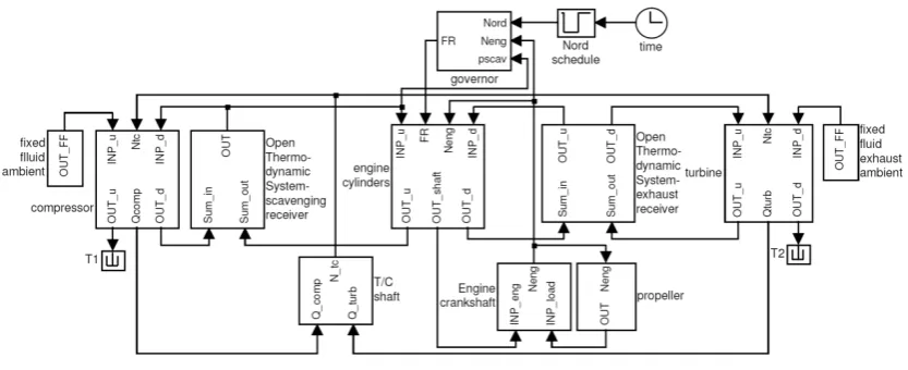
The engine model is implemented in MATLAB/Simulink environment according to a modular approach.

The utilised blocks and connections are shown in Figure 1.

The engine inlet and exhaust receivers are modelled as control volumes, whereas the turbocharger

compressor and turbine are modelled as flow elements. For the engine cylinders a hybrid flow element-

control volume approach is used as explained below. An engine governor controls the fuel flow using a

proportional-integral (PI) controller law with torque and scavenging pressure limiters, whilst the engine load

and the ordered speed are considered input variables to the model. The working fluid (air and exhaust gas) is

considered ideal gas and therefore, the fluid properties depend on gas composition and temperature. For the

calculation of the exhaust gas composition, the following species were taken into account: N2, O2, H2O and

CO2.

2.1 Shafts dynamics

The engine crankshaft and turbocharger shaft rotational speeds are calculated according to the following





π

Sh E P E

Sh

dN

dt I

  



(1)





30

π

T C TC

TC

dN

dt I

 



(2)

where ISh represents the total inertia of the engine-propeller shafting system including the engine crankshaft,

gearbox, shafting system, propeller and entrained water inertia, τ represents the torque and N the shaft speed,

whilst subscripts E, P, T, C and TC represent the engine, propeller, turbine, compressor and turbocharger

elements, respectively. The shafting system efficiency is considered a function of the engine load as

described in [43].

2.2 Turbocharger components

The compressor is modelled using its steady state performance map, which provides the interrelations

between the compressor performance variables, in specific: corrected flow rate, pressure ratio, corrected

speed and efficiency. Turbocharger speed and pressure ratio are considered input to the model, which allows

the computation of the corrected flow rate and efficiency through interpolation [27]. The turbocharger shaft

speed is calculated in the turbocharger shaft block, whilst the compressor pressure ratio is calculated

according to the following equation, which accounts for pressure losses in the air cooler and filter:

IR AC C

amb AF

p p

pr

p p

  

  ₍₃₎

where prc, represents the compressor pressure ratio and the subscripts IR, AC, AF and amb represent the inlet

receiver, air cooler, air filter and ambient conditions, respectively. The pressure in the inlet receiver and the

ambient pressure are taken from the inlet receiver and fixed fluid elements, connected downstream and

upstream of the compressor element, respectively. The air filter and air cooler losses are considered to be

proportional to the square of the compressor air mass flow rate.

The temperature of the air exiting the compressor is calculated according to the following equation, which

was derived by using the compressor efficiency definition equation [44]:

 









, , 1 a 1 /

C d C u C C

T T  pr     

(4)

where Tc,d, Tc,u, γa andηc represent the compressor outlet and inlet temperature, air heat capacities ratio and

compressor efficiency, respectively. The compressor absorbed torque can subsequently be calculated





30 / ( )

C m hC C d hC u NTC

    

(5)

The specific enthalpy of the air exiting the compressor is calculated by using the respective temperature

calculated from eq. (4), whereas the specific enthalpy of the air entering the compressor is taken from the

fixed fluid element connected upstream.

The temperature of the air exiting the air cooler is calculated based on the air cooler effectiveness

definition equation [44]:

, (1 )T,

AC d W C d T T  

(6)

where ε and Tw represent the air cooler effectiveness and the cooling water inlet temperature, respectively.

The air cooler effectiveness is assumed to be a polynomial function of the air cooler air mass flow rate. The

specific enthalpy of the air exiting the air cooler is calculated by using the respective temperature as derived

by eq. (6)

The turbine is modelled using its swallowing capacity and efficiency maps, which allow the calculation of

turbine flow rate and efficiency through interpolation. The turbine pressure ratio is calculated according to the

following equation, by taking the exhaust pipe pressure losses into account, which are considered to be

proportional to the square of the exhaust gas flow rate:

ER T

amb ep

p pr

p p



 

(7)

where the subscripts ER and ep refer to the exhaust receiver and the exhaust pipe, respectively. The exhaust

gas outlet temperature is calculated by using the turbine efficiency definition equation [44], whereas the

turbine torque is derived by using the following equation:





30 / ( )

T m hT T hT NTC

    

(8)

The specific enthalpy of the exhaust gas exiting the turbine is calculated by using the respective

temperature, whereas the specific enthalpy of the exhaust gas entering the turbine is taken from exhaust

receiver element connected upstream.

2.3 Inlet and Exhaust receivers

The flow receiver elements (inlet and exhaust receiver) are modelled using the open thermodynamic

system concept [44–46]. By applying the mass and energy conservation laws considering that the working

neglecting the dissociation effects and the kinetic energy of the flows entering/exiting the receivers, the

following equations are derived for calculating the mass and temperature time derivatives:

in out

dm

m m

dt     ₍₉₎

   

ht in out v

dm

Q mh mh u

dT _dt

dt mc

  



 _{ }

(10)

where and represent the mass and energy flow rates and the subscripts in and out denote the flows

entering and exiting the flow receiver, respectively. Heat transfer is not considered for the inlet receiver,

whereas for the case of exhaust receiver, the heat transferred from the gas to the ambient is estimated by

using the temperature difference, the exhaust receiver surface and the heat transfer coefficient. The latter is

calculated using a typical Nusselt-Reynolds number correlation for gas flowing in pipes [47]. The pressure of

the working medium contained in the engine receivers is calculated by using the ideal gas law equation.

The properties of the working medium (air for the inlet receiver; exhaust gas for the exhaust receiver) are

calculated by using the respective temperatures and the equivalence ratio for the case of exhaust receiver.

2.4 Engine cylinder modelling

The engine cylinders are considered to be a hybrid element that combines functionalities from the mean

value and the zero dimensional approaches as explained below.

2.4.1 Open cycle modelling

The open part of the engine cylinders cycle (gas exchange period) is modelled by using the mean value

approach. In this respect, the mass and energy flows entering and exiting the cylinders are calculated in per

cycle basis. The mass flow rate of air entering the cylinders is calculated by considering the pumping mass

flow rate and the scavenging flow rate (during the valve overlap period), as follows:

a pump scav

m





m





m



(11)

The pumping mass flow rate is derived by using the following equation as function of the engine cylinders

volumetric efficiency, the density of the inlet receiver, the engine displacement volume and the engine speed:

60 vol IR D E pump

V N m

k   



(12)

The engine volumetric efficiency of the process is calculated according to the following equation as

suggested in [46] as a function of the engine compression ratio (rc) and the temperature upstream inlet valve,

which is considered equal to the temperature in the inlet receiver (and therefore is taken from the inlet

receiver block):

5

1 313 ( 273.15) 6 c IR vol c IR r T r _T  

 _{ } (13)

The scavenging mass flow rate is calculated according to the following equation, which was derived

assuming subsonic flow consideration through the valves [44,45] during the valve overlapping period:

1 2

2 1

IR IR IR

scav d eq

ER ER a IR

p p p

m c A

p p R T                 _  _     (14)

The equivalent cylinders flow area (Aeq) can be estimated using the instantaneous area variations for an

engine cycle of the intake and exhaust valves, as follows:

0 2 2

( ) ( )

d

( ) ( )

cy

cyl IV EV eq

cy _{IV EV}

z A A

A A A      _{ }  



The mass flow rate of the exhaust gas exiting the engine cylinders is calculated as the sum of the air and

fuel flows entering the cylinders, i.e.:

e a f

m m m











The fuel mass flow is calculated by using the injected fuel mass per cylinder and per cycle, which is

regarded as a function of engine fuel rack position. The latter is adjusted by the engine governor and it us

modelled using a proportional-integral (PI) controller law with torque and scavenging pressure limiters, as

commonly used by engine manufacturers for protecting the engine integrity during fast transients [48].

The exhaust gas equivalence ratio is calculated by using the fuel and air flow rates as well as the fuel-air

stoichiometric ratio, which is a property of the utilised fuel. This is fed to the exhaust receiver and used for

calculating the exhaust gas properties.

The energy rate entering the engine cylinders is calculated by using the air mass flow rate derived from eq.

(11) and the specific enthalpy of air, which is taken from the inlet receiver block. The energy rate exiting the

engine cylinders is calculated by applying the energy balance to the cylinders block, as described in the

following equation:

e f comb a w

For taking into account the effects of incomplete combustion, the combustion efficiency is considered a

function of exhaust gas equivalence ratio. The engine cylinders indicated power and heat transfer rate for the

entire engine cycle are required in eq. (17) and therefore, this calculation is performed for each engine cycle.

Eq. (17) can be compared to the way that the respective parameter is calculated for the case of MVEM, which

is based on the fuel energy chemical proportion in the exhaust gas exiting the engine cylinders. The latter has

to be provided as input and needs to be calibrated based on the available experimental data [29,49].

2.4.2 Closed cycle modelling

The closed part of the cylinder cycle is modelled according to a 0-D approach by considering the following

phases: compression, injection, combustion and expansion. Each phase is modelled by considering the mass

and energy conservation equations along with the ideal gas state equation, the working fluid properties and

the appropriate submodels to represent the engine combustion and heat transfer.

By considering the energy conservation neglecting the kinetic energy and assuming for the working

medium ideal gas and homogeneous mixture, the state of which can be determined by using its pressure,

temperature and composition, the following equation is derived for calculating the cylinder working internal

energy time derivative:

f

w

dQ dV dm

p Q u

du _{dt dt dt}

dt m

  





(18)

In the above equation, the heat release rate (dQf/dt) is calculated by using the combustion model described

below. The properties of the working medium (either air or exhaust gas) were calculated as functions of

temperature and gas composition [45]; dissociation effects were not taken into account. The cylinder volume

and the volume derivative were calculated based on the engine kinematic mechanism particulars [45].

The ignition delay is calculated by using the following equation as proposed by Sitkei [50]:

7800 7800

3 6.9167 0.7 6.9167 1.8

6 10 RT(1.0197 ) RT(1.0197 )

id N aid b eid p c eid p

     

   _   _

  (19)

where N represents the engine speed in r/min, T the gas temperature in K, and p the pressure inside the

cylinder in bar; aid, bid, and cid are constants estimated as suggested in [51] for large Diesel engines.

Combustion is modelled according to a Vibe curve, which is often referred to as a good approximation for

, ( 1) SOC comb m a f SOC f tot comb dQ

Q a m e

d            _ _        _{  } 

  ₍₂₀₎

where  represents the crank angle in degrees, Qf the heat release, combthe total combustion duration and

SOC

 the start of combustion. The value of the constant a is related to the combustion efficiency, and was

assumed equal to 5 as suggested in [53]. Constants m and combare calibrated at the engine reference point

and are updated at the other operating points according to the following equations, as proposed by Woschni

and Anisits [51]:

,

comb comb b

a ref comb comb ref

ref N N              _ _

    ₍₂₁₎





, m

m m c

a b

ref

id IVC

ref

id IVC ref

N m

m m m m

N m               _{ } _    

    ₍₂₂₎

The constants acomb, bcomb, am, bm and cm are regarded as the model calibration parameters, since they can

sensibly differ amongst various engines types and sizes as reported in [51].

The cylinder heat losses (from working medium to cylinder walls) are calculated using the standard

equation for convective heat transfer assuming a constant value for the cylinder walls temperature:

( )

w cyl w

Q hA T T ₍₂₃₎

The average of cylinder heat losses over one engine cycle was calculated and used in eq. (17). For

calculating the heat transfer coefficient from cylinder gas to wall, the Woschni correlation was used [19,51]:

0.8 0.8 0.2 0.53 127.93

h_ p w d T

(24)

where p represents the cylinder pressure in bar, d the cylinder diameter in m, T the cylinder gas temperature

in K and w is a representative velocity that takes into account the mean piston speed and the combustion

induced turbulence.

Eq. (18)-(24) along with the mass conservation and the ideal gas equations form a system of equations that is

solved for each crank angle step of the closed cycle from IVC to EVO. A variable time step approach was

used with the upper limit equal to 2 degrees crank angle.

2.4.3 Calculation procedure

block components and the other engine elements are shown in Figure 2. The input from the adjacent elements

include: the pressure, temperature and specific enthalpy from inlet receiver; the pressure from the exhaust

receiver; the rack position from governor; and the engine speed from shaft element. The injected fuel amount

is calculated by using the rack position and subsequently it is used along with the engine speed for the

calculation of the fuel mass flow rate. Using the MV approach, the cylinders air and exhaust gas mass flow

rates as well as the energy flow of the air entering the engine cylinders and the equivalence ratio of the

exhaust gas exiting the cylinders are calculated.

Based on the inlet receiver pressure and temperature, the initial cylinder pressure and temperature for the

start of closed cycle are derived. In specific, the cylinder pressure at the IVC is assumed equal to the inlet

receiver pressure; the temperature at IVC is assumed equal to the inlet receiver temperature increased by a

reasonable value in order to account for the mixing with the residual exhaust gas [54]; the working medium at

IVC is assumed to be air, since the residual exhaust gas fraction is generally small in four-stroke marine

Diesel engines [20] and its influence on the prediction of the trapped gas during the compression phase is

therefore limited.

The additional input of the 0-D model includes the engine geometry and the model constants as well as

the crank angle at IVC and the crank angle step. The pressure, temperature, heat release and heat loss are

calculated for the closed cycle and the total closed cycle work and heat loss are derived. The output of the

MV and 0-D models are combined for calculating the remaining cylinder performance parameters including

the energy flow of the exhaust gas exiting cylinders, the indicated power, the friction power, the brake power,

and torque, the brake specific fuel consumption and the engine brake efficiency.

In specific, the indicated mean effective pressure is derived by elaborating the calculated cylinder pressure

diagram for the closed cycle and taking into account the pumping work for the open cycle; the latter is the

product of the cylinder pressure difference and the engine cylinders displacement volume. The engine brake

mean effective pressure is calculated by subtracting the friction mean effective pressure from the indicated

mean effective pressure, whereas the engine torque is calculated using the brake mean effective pressure and

engine cylinders displacement volume. Several correlations were proposed for the modelling of friction mean

effective pressure. In this study, the mean of the correlations proposed by Chen and Flynn [55] and McAuley

et al. [56], which are both linear functions of engine speed and maximum pressure, was used.

Then, the calculated parameters are forwarded to the adjacent engine components as shown in Figure 2.

exhaust gas mass and energy flow rates along with the gas equivalent ratio are advanced to the exhaust

receiver element; and the engine torque is transferred to the shaft element.

2.5 Model set up procedure and constants calibration

For setting up a new engine morel, the subsequent steps are followed:

• Selection and connection of the blocks representing the engine components.

• Insertion of the required input data in each block.

• Preliminary calibration of the model constants for a reference point.

• Fine tuning of the model constants.

The following input data are needed to set up the model: the engine geometric data, the equivalent area

of the cylinder intake and exhaust valves, the steady state compressor and turbine performance maps, the

constants of engine combustion model, the propeller loading and the ambient conditions. For integrating the

time derivatives of the model governing equations, initial values are also required for the following variables:

the engine/propeller and turbocharger rotational speeds, the temperature and pressure of the working medium

contained in the engine receivers.

The three main engine parameters describing the combustion (Vibe curve parameters) are not usually

known beforehand and need to be determined through a training procedure. The combustion model was

initially calibrated versus shop trials performance data for the engine maximum continuous rating (MCR)

point, which was considered as the reference point, in order to determine the range for Vibe curve parameters

Δϕcomb,ref and mcomb,ref. The parameters defining the shape of the heat release rate function in other engine

operating points (eq. 21-22), are calibrated by using the full set of shop trial data. The values proposed by

Woschni-Anisits for large two-stroke Diesel engines and heavy duty four-stroke engines are used as

boundaries. Finally, all combustion model parameters were fine-tuned at the full engine model. This

multiple-level calibration procedure allows for reducing the model set-up time. All calibration steps were performed

using a Genetic Algorithm, which had been previously utilized [31] providing promising results.

3. Test case

The four-stroke marine Diesel engine MaK 8M32C was simulated using the described combined MV-0D

engine model. The MaK 8M32C is a four stroke, eight cylinders in line, turbocharged engine; one

main engine characteristics as well as the required input data were gathered from the engine project guide

[57].

Medium speed engines of this size are normally used as propulsion and auxiliary engines in RoRo vessels,

small tankers and bulk carriers. For the present study, the propulsion plant arrangement of a handymax size

chemical tanker was selected for testing the model predictive ability. In this arrangement, two engines

provide power to the ship propeller and one shaft generator unit; a gearbox of two inputs (the shaft of each

engine) and two outputs (shaft generator, propeller) is used as shown Figure 3. The propeller is of the

controllable pitch type, whereas the engine/propeller gearbox ratio is 5.68. Additionally to the shaft generator,

the vessel power plant includes two diesel generator sets having a rated power of 690 kWe for providing the

required electrical power in cases where the propulsion engines or the shaft generator are not in operation.

The main characteristics of the vessel and each propulsion engine are summarized in Table 1.

4. Model set up and validation

The engine model was set up providing the required input data, including engine geometric data,

turbocharger compressor and turbine steady-state performance maps, model constants and initial conditions.

For the investigated engine, the engine shaft speed was used as control variable for the PI regulator and

therefore, its initial value was set equal to the desired engine speed value. For the case of the receivers’

pressure and temperature, polynomial regressions as a function of engine load were used to estimate the

initial conditions derived from the shop trial measurements. The fuel was assumed to be of the marine diesel

oil (MDO) type with a lower heating value equal to 42.4 MJ/kg as this fuel type was used in the engine trials.

This value was also used for calculating the engine brake specific fuel consumption (bsfc) presented below.

The combustion model constants were calibrated as described in Section 2.5 by using the engine

performance data from engine shop trials. Measurements for the engine efficiency and the exhaust gas

temperature at turbine inlet at 100% load were used for training the model, whereas measurements at other

loads (50%, 85%, and 110% of the engine MCR) were used for the model validation. The relative errors for

the brake specific fuel consumption and the exhaust gas temperature at turbine inlet were used in both cases

for determining the objective function used by the genetic algorithm, as described by the following equation:

,

obj i rel i i

f 



The calibrated combustion model parameters are shown in Table 2. It must be noted that the Δm parameter

at low loads.

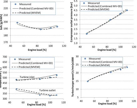
The steady state simulation results at constant engine speed (equal to 600 r/min) are presented in Figure 4.

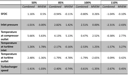
In addition, Table 3 contains the obtained percentage relative errors between the parameters calculated using

the MVEM, the combined MV-0D model and the respective measured data. The results presented in Table 3

show that the combined model presented herein exhibits reasonable accuracy over the entire engine operating

range. It can be inferred that the performance of the two models (MVEM and combined MV-0D) are

comparable. The combined MV-0D model shows a slight tendency of underestimating engine brake specific

fuel consumption at 50% load, with an error which is however lower than the standard tolerance employed by

the marine engine manufacturers. The obtained agreement between the predicted and measured values for the

MVEM is better, which is attributed to the effective calibration process for this model. However, it must be

noted that the MVEM is placed closer to a black-box model than the proposed combined MV-0D alternative

[57].

5. Model application

Having validated the engine model, it was possible to use it in order to investigate various engine

operating cases. The steady-state performance over a range of engine loads from 50% to 110% (using 5%

load increase step) at constant engine speed (600 r/min) was first examined. The derived engine parameters

including the brake specific fuel consumption (bsfc), the turbocharger speed, the pressure at compressor

outlet and the exhaust gas temperature at turbine inlet and outlet are shown in Figure 4. Values predicted by

the combined model are shown, along with the respective predictions obtained using the MVEM model as

well as the measured values from shop trials at 50%, 85%, 100% and 110% loads. Once again, good

agreement between measured and predicted results by the combined MV-0D and the mean value models can

be observed throughout the investigated engine operating envelope. It is inferred from the engine parameters

presented in Figure 4, the engine was optimised at the high loads region, since the minimum brake specific

fuel consumption is obtained at 85% load and the minimum turbine outlet temperature is observed at 100%

load. This reflects the market conditions when the ship was designed and built, when slow-steaming and low

speed operations were not considered as a possible operating mode.

Figure 5 shows the cylinder pressure diagrams, which can be calculated by using the proposed combined

MV-0D approach and are not available for the case of the MVEM. The cylinder maximum pressure at 100%

relative percentage error that was finally obtained for this parameter at MCR point was 0.8%. As the

in-cylinder pressure variation can be predicted by the combined model, this model can be used in the cases were

this feature is needed, as an alternative to a 0-D model, which is more complex and computationally

demanding. Figure 6 shows the calculated heat losses to cylinder walls, charge air cooler and exhaust gas for

various engine loads. Experimental values for the engine heat losses were not available for validation.

Therefore, the results from the proposed combined model are compared with the results from the MVEM;

the maximum relative percentage differences for the energy flows of the charge air cooler and the exhaust

gas were found to be 9.4% and 7.3%, respectively. The prediction of heat losses to the cylinder walls is a

result of the combination of the MV and 0-D models, since the calculation of in-cylinder temperature over

the closed cycle allows for the utilization of the Woschni correlation for the estimation of cylinder heat

losses. These results can be of particular interest in the design and optimization of engine cooling and waste

heat recovery systems.

5.1. Engine brake specific fuel consumption map

For the investigated engine, no measurements or data were available at speeds different than the nominal.

By using 0-D or the combined model proposed in this work, the estimation of the effect of engine speed on

the engine efficiency and on the other parameters can be provided. MVEMs, however, are intrinsically unable

to take this effect into account, since the in-cylinder processes are not modelled. The proposed model can

provide the required fidelity in the prediction of the influence of engine speed on efficiency.

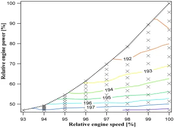
Figure 7 shows the results from the application of the model to predict the engine brake specific fuel

consumption within the engine power-speed region. It must be noted that the operating envelope of the

investigated engine is very narrow and therefore it allows for only limited reduction in engine speed. As

expected, the engine speed has the highest impact on engine efficiency in the region close to the upper

boundary of the operating envelope, whilst at lower loads the engine efficiency becomes rather insensitive to

the engine speed variation. However, a slight bsfc improvement (1-2 g/kWh) could be achieved by operating

at an optimal engine speed, which provides the minimum bsfc at each engine load. The utilization of the

proposed model allows for the extension of the efficiency map to the whole engine operating envelope, which

is not available from the engine shop tests, the sea trials or the engine project guide. Thus, the more detailed

modelling approach followed for the development of the proposed combined model, when compared to mean

for which the model constants have been calibrated.

5.2. Variable Geometry Turbine effects on engine performance

The limited size of the allowed speed range for the test-case engine renders a strong limitation for

considerable efficiency improvement of the vessel overall propulsion train, since optimal operations at a

lower ship speed (e.g. reduction from 15 knots to 12 knots) would require a reduction of the engine speed,

which is not permitted for the investigated engine [57]. Reducing turbine area can improve the engine

charging process at low loads and consequently can reduce the exhaust gas temperatures. Therefore it is a

widely recognized method for broadening the turbocharged engines operating envelope at low loads [15].

Since measurements with a different turbocharger turbine area were not available, the combined model can be

used to predict the engine behaviour in this case. On the contrary, MVEMs are not able to fully simulate the

effect of increased air charge pressure on engine efficiency and in-cylinder performance parameters. The

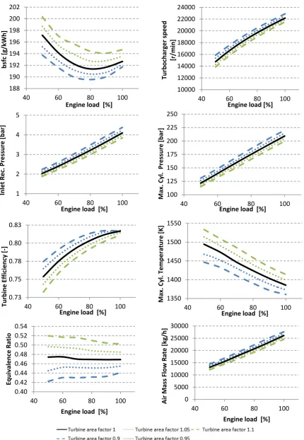
model derived results using turbine geometric area values in the range from 90% to 110% of its original value

for fixed engine speed operation (600 r/min) are presented in Figure 8.

Reducing turbine inlet area has the main impact of increasing the pressure at turbine inlet, thus providing

more exhaust gas energy to the turbine, which increases the turbocharger speed and as a result, the engine

inlet receiver pressure. The latter increases the maximum cylinder pressure, which has as a consequence the

increase of the engine efficiency and therefore, the decrease of the brake specific fuel consumption. The

opposite happens in the case of increasing the turbine geometric area. The above described behaviour is

clearly shown in Figure 8. However, if the turbine geometric area decrease is too large, the engine efficiency

may deteriorate and the maximum cylinder pressure might increase above the allowed limit.

The effect of a higher air mass flow rate is also shown in Figure 8, where the equivalence ratio is shown for

different values of turbine inlet area. The increase of the equivalence ratio results in a decrease of the peak

temperatures and as a result, in lower engine thermal loading. This behaviour, also shown in Figure 8, can

potentially lead to an extended operational envelope towards lower loads for a given engine speed.

As it was explained above, reducing the inlet turbine area causes an increase in turbocharger speed. At low

engine loads, however, the turbocharger speed is far from its high limit and therefore, it should not present a

confining factor. In this case, the engine in-cylinder pressure level increases at low loads, which results in a

5.3 Propulsion plant variable speed operation

The model ability to predict the engine performance at different loads and speeds was employed in order

to test the potential for improving the operational efficiency of the investigated vessel propulsion plant. The

two alternative operational modes that are compared are as follows: (a) the propulsion plant operates with

constant engine speed equal to 600 r/min and the shaft generator is used to supply the required electrical

power; and (b) the diesel generator sets are used for covering the ship electrical power demand, which allows

for operations at variable propeller and engine speeds. The required ship electrical power was set to 400 kWe

based on available measurements from on-board power system.

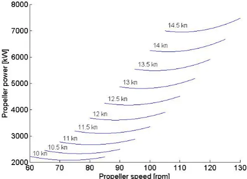
The rationale for operating at variable propeller speed is attributed to the fact that the propeller efficiency

depends on its rotational speed as it is shown in Figure 9. Hence, operations at constant propeller speed,

although allowing for the generation of the ship electrical energy at higher efficiency, lead to lower propeller

efficiency at ship speeds lower than the design speed.

The two alternative operational modes were tested for various ship speeds in the range from 10 to

14 knots. The ship resistance was regarded as a polynomial function of the ship speed, whereas the propeller

efficiency was derived using the Wageningen series polynomials as described in [58]. The proposed

combined MV-0D engine model was used to predict the engine performance under fixed or variable engine

speed operating conditions. The following input was additionally used for modelling the two considered

cases: i) gearbox efficiency at full load 98%; ii) shafting system efficiency at full load 99%; iii) shaft

generator efficiency at rated power 95%; iv) diesel generators bsfc 210 g/kWh (one diesel generator set

operates at 57% load for generating the required electrical power); v) electric generator efficiency at the

considered operating point equal to 95%. The rated efficiencies for the gearbox, shafting system and shaft

generator are corrected as proposed in [43] for operation at part loads.

The following additional equations were used for the propulsion system modelling under steady state

operating conditions:

1 2

( )

GB PE PE Psh PSG

    (26)

/ /

SG el SG sh p sh

P P  and P P  (27)

/ AE AE el EG

m bsfc P  (28)

The derived results including the propeller power, the engine bsfc for each operating engine, the engine

load and speed, the total fuel flow demand for the operating propulsion engines and diesel generator sets, are

propeller power in this operating mode is required at the entire investigated speed range. It must be noted that

for constant engine speed operation (case a), two engines need to operate for ship speed greater than

10.4 knots, whereas for ship speed lower than this, one engine can cover the required total power demand

(propulsion and electrical). For the variable engine speed operation (case b), the break point for reducing the

number of operating engines from two to one is at 11.8 knots. Therefore, in both cases the maximum engine

bsfc point is observed at the break points, since the load of the operating engine increases after switching off

one engine unit and consequently the engine bsfc decreases till the engine load reaches the operating point

having the minimum bsfc. The engine bsfc is generally lower when operating at variable engine speed, which

depends on a combination of the effects of the higher engine load and the lower engine speed.

The calculated total fuel flow demand demonstrates that fuel consumption savings in the range between

1% and 6% can be obtained when operating at variable engine speed even if the ship electrical power is

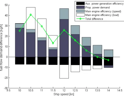
covered by the less efficient diesel generator sets. Figure 11 shows a breakdown of the different contributions

to the total fuel flow demand, which can explain the observed fuel savings. The largest part of the fuel

improvement at the variable engine speed mode is attributed to the reduction of propeller power (as a

consequence of the propeller efficiency increase). The engine running at different loads, as a consequence of

the varying power demand, contributes positively or negatively on the fuel flow demand depending on the

ship speed. It must be noted that the contribution at lower ship speeds, which is of the highest interest given

the current slow-steaming operations used by shipping companies, is beneficial to reduce the fuel flow

demand. In addition, operating at lower engine speeds also provides a considerable reduction in fuel flow

demand, although this effect is more pronounced at higher ship speeds. As it was expected, the electrical

power generation is substantially more efficient when operating at constant speed by using the shaft

generator.

It can be concluded from the presented case studies that the developed MV-0D engine model can be used

as an alternative to the 0-D models, in studies where varying engine operating conditions in terms of load and

speed prevail. The usage of MVEMs is not recommended as calibration of the model constants in a broader

engine operating envelope is needed unless extensive experimental data are available.

6.

Conclusions

A combined mean-value-zero dimensional model was developed and the simulation of a large marine four

parameters measured during engine shop trials and additionally, they were compared with results obtained by

using a mean value engine model. Then, the model was used to simulate a number of engine operating points

and the results were used for generating the brake specific fuel consumption map in the whole engine

operating envelope. Furthermore, cases with varying the turbine geometric area were simulated, so that the

model usefulness and superiority against mean value models are presented.

The main conclusions derived from the present work are summarised as follows.

The proposed model can be seen as a compromise between the more empirical mean value models and the

more detailed zero dimensional models and can be used in cases where the additional features provided by

the 0-D approach are required. The model set up and calibration is faster than the respective one for the 0-D

models as only the closed cycle of one engine cylinder is additionally modelled. The calibration of the

combustion model parameters is required, which is not too demanding compared with the calibration of the

cylinder sub-model for mean value model that requires access to engine performance data and a considerable

pre-processing phase.

The model execution time is only slightly greater than the one of the mean value model. In addition, the

model prediction capability is quite adequate as it was revealed by the derived parameters comparison against

experimental data. The proposed model predicted parameters were comparable with the respective parameters

obtained by using the mean value model. The model output parameter set is enhanced, as it additionally

includes the in-cylinder parameters, such as pressure, temperature and heat transfer rate. In this respect, the

engine efficiency and brake specific fuel consumption can be reasonably predicted in the whole engine

operating envelope (with varying load and speed) and in cases where the engine settings change (e.g. variable

injection timing and variable geometry turbine).

The model can be used for creating response surfaces for the calculated engine parameters covering the

whole operating envelope. The influence of the engine settings on the engine performance are taken into

account, since the closed cycle is modelled. Therefore, there is no need for recalibrating the engine cylinder

sub-models, as it is required for the mean value models.

The additional case studies of the engine with installed a variable geometry turbine and the vessel

propulsion system that can operate in different operating modes revealed the developed model capability of

predicting the engine and propulsion system behaviours, respectively. Therefore, the model can effectively

assist in the identification of the most efficient engine/propulsion system operations, thus contributing to the

In conclusion, the combined mean value-zero dimensional model can be used in studies where the mean

value model reaches its limitations, especially considering the simulation of electronically controlled versions

of marine engines, as well as for simulating engines equipped with variable geometry turbine turbochargers

and engine operating in an varying range of operating conditions.

REFERENCES

[1]  García‐Martos C, Rodríguez J, Sánchez MJ. Modelling and forecasting fossil fuels, CO2 and 

electricity prices and their volatilities. Appl Energy 2013;101:363–75. 

[2]  Zhang C, Chen X. The impact of global oil price shocks on China’s bulk commodity markets and 

fundamental industries. Energy Policy 2014;66:32–41. 

[3]  Zhang Y‐J, Wang Z‐Y. Investigating the price discovery and risk transfer functions in the crude 

oil and gasoline futures markets: Some empirical evidence. Appl Energy 2013;104:220–8. 

[4]  IMO. Air pollution and energy efficiency‐estimated CO2 emissions reduction from introduction 

of mandatory technical and operational energy efficiency measures for ships. MEPC 63/INF.2 

2011. 

[5]  UNCTAD. Chapter 3: Freight rates and maritime transport costs. Rev. Marit. Transp. 2013, 

2013. 

[6]  Buhaug O, Corbett JJ, Endersen O, Eyring V, Faber J, Hanayama S, et al. Second IMO GHG Study 

2009. London, UK: International Maritime Organization (IMO); 2009. 

[7]  Faber J, Nelissen D, St Amand D, Consulting N, Balon T, Baylor M, et al. Marginal Abatement 

Costs and Cost Effectiveness of Energy‐Efficiency Measures. 2011. 

[8]  Baldi F, Johnson H, Gabrielii C, Andersson K. Energy and exergy analysis of ship energy 

systems‐the case study of a chemical tanker. Proc. 27th Int. Conf. Effic. Cost, Optim. Simul. 

Environ. Impact Energy Syst., Turku, Finland: 2014. 

[9]  Brunner H. Upgrade of Wartsilas Two‐Stroke Engine Portfolio to fulfil the Changing Marine 

Market Requirement. Proc. Congr. Int. Counc. Combust. Engines, Shanghai, China: 2013. 

[10]  Jakobsen SB, S MANDA, Egeberg C. Service Experience of MAN B&W Two Stroke Diesel 

Engines. Proc. Congr. Int. Counc. Combust. Engines, Vienna, Austria: 2007. 

[11]  Mest S, Diesel MAN, Loewlein O, Balthasar D, Schmuttermair H. TCS‐PTG ‐ MAN Diesel & Turbo 

’ s power turbine portfolio for waste heat recovery. Proc. Congr. Int. Counc. Combust. Engines, 

Shanghai, China: 2013. 

[12]  Nielsen RF, Haglind F, Larsen U. Design and modeling of an advanced marine machinery system 

including waste heat recovery and removal of sulphur oxides. Energy Convers Manag 2014;85. 

[13]  Livanos G aA., Theotokatos G, Pagonis D‐N. Techno‐economic investigation of alternative 

[14]  Hou Z, Turbo ABB. New Application Fields for Marine Waste Heat Systems by Analysing the 

Main Design Parameters. Proc. Congr. Int. Counc. Combust. Engines, Vienna, Austria: 2007. 

[15]  Schmuttermair H, Diesel MAN, Se T, Fernandez A, Witt M. Fuel Economy by Load Profile 

Optimized Charging Systems from MAN. Proc. Congr. Int. Counc. Combust. Engines, Bergen, 

Norway: 2010. 

[16]  Ono Y, Industries MH. Solutions for better engine performance at low load by Mitsubishi 

turbochargers. Proc. Congr. Int. Counc. Combust. Engines, Shanghai, China: 2013. 

[17]  Lamaris V, Antonopoulos A, Hountalas D. Evaluation of an Advanced Diagnostic Technique for 

the Determination of Diesel Engine Condition and Tuning Based on Laboratory Measurements. 

SAE Tech Pap No 2010‐01‐0154 2010. 

[18]  Ahmed FS, Laghrouche S, Mehmood A, El Bagdouri M. Estimation of exhaust gas aerodynamic 

force on the variable geometry turbocharger actuator: 1D flow model approach. Energy 

Convers Manag 2014;84:436–47. 

[19]  Kumar S, Kumar Chauhan M. Numerical modeling of compression ignition engine: A review. 

Renew Sustain Energy Rev 2013;19:517–30. 

[20]  Stone R. Introduction to internal combustion engines. Third Edit. Palgrave Macmillan; 1999. 

[21]  Malkhede DN, Seth B, Dhariwal HC. Mean Value Model and Control of a Marine Turbocharged 

Diesel Engine. Powertrain Fluid Syst. Conf. Exhib., San Antonio, USA: 2005. 

[22]  Schulten PJM, Stapersma D. Mean Value Modelling of the Gas Exchange of a 4‐stroke Diesel 

Engine for Use in Powertrain Applications. 2003 SAE World Congr., Detroit, USA: 2003. 

[23]  Grimmelius HT, Boonen EJ, Nicolai H, Stapersma D. The integration of mean value first 

principle Diesel engine models in dynamic waste heat and cooling load analysis. Proc. Congr. 

Int. Counc. Combust. Engines, Bergen, Norway: 2010. 

[24]  Weinrich M, Bargende M. Development of an Enhanced Mean‐Value‐Model for Optimization 

of Measures of Thermal‐Management. SAE Tech Pap 2008:1–1169. 

[25]  Theotokatos GP. Ship Propulsion Plant Transient Response Investigation using a Mean Value 

Engine Model. Int J Energy 2008;2:66–74. 

[26]  Guan C, Theotokatos G, Zhou P, Chen H. Computational investigation of a large containership 

propulsion engine operation at slow steaming conditions. Appl Energy 2014;130:370–83. 

[27]  Theotokatos  G,  Tzelepis  V.  A  computational  study  on  the  performance  and  emission 

parameters mapping of a ship propulsion system. Proc Inst Mech Eng , Part M   J Eng Marit 

Environ 2015;229:58–76. 

[28]  Dimopoulos GG, Georgopoulou CA, Kakalis NMP. Modelling and optimization of an integrated 

marine combined cycle system. Proc. Int. Conf. Effic. Cost, Optim. Simul. Environ. Impact 

Energy Syst., Novi Sad: 2011. 

[29]  Theotokatos G. On the cycle mean value modelling of a large two‐stroke marine Diesel engine. 

[30]  Catania AE, Finesso R, Spessa E. Predictive zero‐dimensional combustion model for di diesel 

engine feed‐forward control. Energy Convers Manag 2011;52:3159–75. 

[31]  Scappin F, Stefansson SH, Haglind F, Andreasen A, Larsen U. Validation of a zero‐dimensional 

model for prediction of NO x and engine performance for electronically controlled marine 

two‐stroke diesel engines. Appl Therm Eng 2012;37:344–52. 

[32]  Asad U, Tjong J, Zheng M. Exhaust gas recirculation – Zero dimensional modelling and 

characterization for transient diesel combustion control. Energy Convers Manag 2014;86:309–

24. 

[33]  Finesso R, Spessa E. A real time zero‐dimensional diagnostic model for the calculation of in‐

cylinder temperatures, HRR and nitrogen oxides in diesel engines. Energy Convers Manag 

2014;79:498–510. 

[34]  Benvenuto G, Campora U, Carrera G, Casoli P. A two‐zone Diesel engine model for the 

simulation of marine propulsion plant transients. Proc. Int. Conf. Mar. Ind., Varna, Bulgaria: 

1998. 

[35]  Kyrtatos NP, Theotokatos G, Xiros NI, Marek K, Duge R, Engineer CS, et al. Transient Operation 

of Large‐bore Two‐stroke Marine Diesel Engine Powerplants: Measurements and Simulations. 

Proc. Congr. Int. Counc. Combust. Engines, vol. 4, Hamburg, Germany: 2001, p. 1237–50. 

[36]  Kyrtatos NP. Propulsion control optimization using detailed simulation of engine/propeller 

interaction. Proc. Sh. Control Syst. Symp., vol. 1, Southampton, UK: 1997, p. 507–30. 

[37]  Xiros NI. Robust control of Diesel ship propulsion. Springer Berlin Heidelberg; 2002. 

[38]  Benson RS. The thermodynamics and gas dynamics of internal combustion engines. Clarendon 

Press; 1986. 

[39]  Eriksson L. Modeling and control of turbocharged SI and DI engines. Oil Gas Sci Technol Rev 

l’IFP 2007;62:523–38. 

[40]  Guzzella L, Onder C. Introduction to Modeling and Control of IC Engine Systems. Berlin: 

Springer; 2009. 

[41]  Livanos G,  Kyrtatos NP, Papalambrou G, Christou, A. Electronic Engine  Control for Ice 

Operation of Tankers. Proc. Congr. Int. Counc. Combust. Engines, No 44, Viena, Austria: 2007.  

[42]  Ding Y, Stapersma D, Knoll H, Grimmelius HT, Netherland T. Characterising the Heat Release in 

a Diesel Engine: A comparison between Seiliger Process and Vibe Model. Proc. Congr. Int. 

Counc. Combust. Engines, Bergen, Norway: 2010. 

[43]  McCarthy WL, Peters WS, Rodger DR. Marine Diesel power plant practices. The Society of 

Naval Architects & Marine Engineers, T&R Bulletin 3‐49. Jersey City, US: 1990. 

[44]  Watson N, Janota MS. Turbocharging the internal combustion engine. Macmillan Press; 1982. 

[46]  Hiereth H, Prenninger P. Charging the internal combustion engine. Vienna, Austria: Springer‐

Verlag; 2003. 

[47]  Bejan A, Kraus AD. Heat Transfer Handbook. Hoboken, US: John Wiley & Sons LTd; 2003. 

[48]  Kyrtatos NP, Theodossopoulos P, Theotokatos G, Xiros NI. Simulation of the overall ship 

propulsion plant for performance prediction and control. MarPower99 Conf., Newcastle upon 

Tyne, UK: The institute of marine engineers; 1999. 

[49]  Meier E. A simple method of calculation and matching turbochargers. Publication CH‐T 120 

163 E. Baden, Switzerland: 1981. 

[50]  Sitkei G. Über den dieselmotorischen Zündverzug. MTZ; 1963. 

[51]  Merker GP, Schwarz C, Stiesch G, Otto F. Simulating Combustion. Berlin Heidelberg: Springer‐

Verlag; 2004. 

[52]  Ding Y. Characterising Combustion in Diesel Engines. TU Delft, 2011. 

[53]  Gogoi TK, Baruah DC. A cycle simulation model for predicting the performance of a diesel 

engine fuelled by diesel and biodiesel blends. Energy 2010;35:1317–23. 

[54]  Ferguson CR, Kirkpatrick AT. Internal combustion engines: applied thermosciences. 2nd ed. 

New York: Wiley; 2001. 

[55]  Chen SK, Flynn P. Development of a compression ignition research engine. SAE Pap 650733 

1965. 

[56]  McAulay KJ, Wu T, Chen SK, Borman GL, Myers PS, Uyehara A. Development and Evaluation of 

the Simulation of the Compression‐Ignition Engine. SAE Tech Pap 1965;650451. 

[57]  MaK. M32C Project Guide ‐ Propulsion 2013. 

[58]  Carlton J. Marine propellers and Populsion. 3rd ed. Butterworth‐Heinemann. Oxford; 2012. 

Nomenclature

Symbols Subscripts

area (m2_{) a air}

BMEP brake mean effective pressure (bar) amb ambient

bsfc brake specific fuel consumption (g/kW h) air cooler

cd discharge coefficient AE Auxiliary engines

specific heat at constant volume (J/kg K) air filter

d Cylinder bore (m) comb combustion

specific enthalpy (J/kg); heat transfer

coefficient (W/m2 _K) corrected

HR Heat release rate (J/deg CA) cy cycle

Energy flow (W) cylinder

I Polar moment of Inertia (kg m2_{) compressor} fuel power heating value (J/kg) downstream Coefficients; revolutions per cycle engine

mass (kg) e exhaust gas

mass flow rate (kg/s) el electrical

rotational speed (r/min) exhaust pipe

pressure (Pa) equivalent

pressure ratio exhaust receiver

P power (W) EV exhaust valve

heat transfer (J) EVO Exhaust valve open

heat transfer rate (W) f fuel

gas constant (J/kg K) GB gearbox

rc compression ratio ht Heat transfer

time (s) id ignition delay

temperature (K) in inlet

specific internal energy (J/kg) IR inlet receiver

V Volume IV inlet valve

VD Engine displacement volume [m3] IVC inlet valve closing

w Velocity (m/s);weight factors (-) ME Main engines

W Work (J) outlet

number of engine cylinders pump pumping

Greek symbols P propeller

ratio of specific heats ref reference

Δ difference scav scavenging

Crank angle difference (deg) SG Shaft generator ∆ _{engine cycle duration (deg) shafting system}

ε Air cooler effectiveness SOC start of combustion

Efficiency T turbine

λ  Air-fuel equivalence ratio (-) turbocharger

  density (kg/m3_{) tot total}

 crank angle (deg) u upstream

torque (Nm) vol volumetric

  w wall

  W Cooling water

List of Figures captions

Figure 1: Matlab/Simulink implementation of marine Diesel engine model

Figure 2: Graphical representation of the interconnections between the combined MV-0D model and the other engine model elements

Figure 3: Schematic representation of ship power plant

Figure 4: Steady-state simulation results and comparison with shop trials data

Figure 5: Combined MV-0D model calculated cylinder pressure diagrams for various engine loads

Figure 6: Calculated cooling power and exhaust gas thermal power versus engine load

Figure 7: Engine efficiency map. X marks show the points where the engine efficiency has been calculated using the proposed model. Iso-efficiency lines have been produced through triangulation.

Figure 8: Combined MV-0D model results for studying the influence of variable turbine area on the engine performance parameters

Figure 9: Propulsion power demand as a function of ship speed and propeller rotational speed for the case study ship considering operation with 15% sea margin

Figure 10: Derived parameters for the case study ship versus ship speed for constant and variable engine speed operations

Figure 11: Breakdown of fuel flow demand difference versus ship speed (Positive values refer to higher fuel flow demand in the fixed engine speed case)

List of Table captions

Table 1: Main parameters for the case study vessel and her propulsion engines

Table 2: Combustion model parameters. Note: * refers to the suggested values for large two-stroke engines; ** refers to the suggested values for heavy duty four-stroke engines; both from [51]

Figure 1: Matlab/Simulink implementation of marine Diesel engine model

Figure 2: Graphical representation of the interconnections between the combined MV-0D model and the other engine model elements

Output

MV

‐

0D

model

Exhaust

Receiver

Governor

Shaft

Open

cycle

MVEM

Closed

cycle

0

‐

D

model

Initial

conditions

Engine

geometry

Model

constants

CA

,

CA

step

, , , a a e

m H m  



, , , , .

w

p T HR Q W vs CA

 

, , , , , e i f b

E

H P P P

bsfc





, IR IR

p T

,

, ,

E f cy f

N m m

E

N

r

x

ord

N

Inlet

Receiver

load



Cylinder

Block

, a a

m H  m H_e, _e,



, , IR IR a

Figure 3: Schematic representation of ship power plant

Figure 4: Steady-state simulation results and comparison with shop trials data

170 180 190 200 210 220 230

40 60 80 100 120

bs fc   [g /k W h ]

Engine load [%]

Measured

Predicted (Combined MV‐0D) 

Predicted (MVEM)

1.0 1.5 2.0 2.5 3.0 3.5 4.0 4.5 5.0 5.5

40 60 80 100 120

C o m p re sso r   ou tl e t   p re ssu re   [b ar ]

Engine load [%]

Measured

Predicted (Combined MV‐0D) Predicted (MVEM)

300 350 400 450 500 550 600 650 700

40 60 80 100 120

Te m p er at u re   [° C ]

Engine load [%]

Measured

Predicted (Combined MV‐0D) Predicted (MVEM)

Turbine inlet

Turbine outlet

5 10 15 20 25 30

40 60 80 100 120

Tu rb o ch a rg e r   sp eed   [r /m in ]x 1000

Engine load [%]

Measured

Figure 5: Combined MV-0D model calculated cylinder pressure diagrams for various engine loads

Figure 6: Calculated cooling power and exhaust gas thermal power versus engine load 0

50 100 150 200 250

0 45 90 135 180 225 270 315 360

Pressure

[bar]

Crank Angle [deg]

50% Load

85% Load

100% Load

0 500 1000 1500 2000 2500 3000 3500 4000

40 60 80 100 120

Thermal

power

[kW]

Engine load [%]

Cylinder walls (Combined MV‐0D)

Charge air cooler (Combined MV‐0D)

Exhaust gas (Combined MV‐0D)

Exhaust gas (MVEM)