Adaptive Exploration based Whale Optimization for Image Segmentation Based on Variable Parametric Error

(1)

International Journal of Innovative Technology and Exploring Engineering (IJITEE) ISSN: 2278-3075, Volume-8, Issue- 6S4, April 2019



Abstract: Image segmentation is the process of splitting an image into numerous segments. Its major purpose is to change or simplify the image, which could be more significant and simpler to examine. However, it does not execute well while segmenting complex images with non-homogeneous parts. In this paper, a hybrid image segmentation model with the aid of Active Contour and Graph cut techniques is proposed. Moreover, it extracts the mutual information from two adopted segmentation schemes, and subsequently, the high-intensity and low-intensity pixels of resultant images are grouped by Fuzzy Entropy Maximization (FEM) method. A modified optimization algorithm termed as Adaptive Exploration based Whale Optimization (AEW) is used for solving the FEM problem. The performance of the proposed Active contour Graph cut Fuzzy Entropy-based Segmentation(AGFES), (AEW-AGFES) is algorithmically analyzed in terms of various performance measures to substantiate its effectiveness.

Index Terms: Adaptiveness; Whale Optimization; Image segmentation; Active contour; Graph cut technique; Fuzzy Entropy Maximization Nomenclature

Acronyms Descriptions FCM Fuzzy C-Means

GM Gaussian mixture FPR False Positive Rate FNR False Negative Rate NPV Net present Value FDR False Discovery Rate

MCC Matthew’s Correlation Coefficient

I. INTRODUCTION

Image segmentation [1] [2] [23] [24] remains a challenging issue in computer vision with a variety of appliances. The aim of segmentation is to separate an image into areas of homogeneous features, which refers to the objects parts or objects. On considering the traditional schemes, unsupervised image segmentation [3] [4] has been one of the extensively deployed techniques. The inspiration of this scheme was to split an input image into a compilation of blocks and subsequently, it clusters the blocks in relation

Revised Manuscript Received on April 12, 2019.

M. Jogendra Kumar, Department of Computer Science and Engineering, Gandhi Institute of Technology and Management, GITAM (Deemed to be University), Vishakhapatnam, A.P, India

Dr. G.V.S Raj Kumar, Department of Information Technology, Gandhi Institute of Technology and Management, GITAM (Deemed to be University), Vishakhapatnam, A.P, India

Dr. K.Naveen Kumar, Department of Information Technology, Gandhi Institute of Technology and Management, GITAM (Deemed to be University), Vishakhapatnam, A.P, India

Dr.Y.Srinivas, Department of Information Technology, Gandhi Institute of Technology and Management, GITAM (Deemed to be University), Vishakhapatnam, A.P India

with certain image features for attaining segmentation outcomes [5] [6] [7]. Conventional characteristics namely, co-occurrence, energy, moment were established and extensively implemented in diverse fields, however, the outcomes are not much remarkable in segmentation appliances [8] [9].

The experimentation exposed that the distribution of image deviations characterizes the contents of the image and shows potential outcomes in classification and retrieval [10] [11]. On the other hand, the distributions are generally high-dimensional that formulates them to less proficient in real time appliances. Therefore discovering an effectual arithmetical model for demonstrating such image deviations is significant and essential. From its initiation, FEM has attained great consideration from experts on these techniques [12] [13]. FEM the renowned clustering technique [14] [15], and its improved models were executed as authoritative tools due to its fast convergence, performance and simplicity [16] [17]. In the previous decades, several reseraches have been undertaken on image segmentation using different techniques. Generally, FEM could attain excellent segmentation accuracy while dealing low or no noise. However, the segmentation [18] [19] outcomes worsen rapidly with the increase in image noise level. For minimizing the worse impacts of noise in fuzzy approach, the better solution is to carry out “image denoising” on the smoothened image.

This paper contributes a hybrid image segmentation approach using Active Contour and Graph cut techniques. In this paper, the high-intensity and low-intensity pixels of the mutual informative image are grouped by FEM scheme. Here, a modified optimization technique named as AEW is deployed for resolving the optimization problem in FEM. The performance of the adopted AEW-AGFES is further algorithmically examined with respect to different performance measures for validating its efficiency. The paper is organized as follows. Section II portrays the literature work. Section III explains the adopted image segmentation procedure, and Section IV explains the adopted contribution of image segmentation. Section V discusses the experimental results, and Section VII concludes the paper.

Adaptive Exploration-based Whale Optimization

for Image Segmentation Based on Variable

Parametric Error

(2)

VARIABLE PARAMETRIC ERROR II. LITERATUREREVIEW

Related works

In 2019, Choy et al. [1] have introduced a new fuzzy-based image segmentation technique. Here, probability model was established for portraying the variations of image distributions on the basis of bit-plane dependencies and probabilities among the bit-planes. The conventional image segmentation models demonstrates that the distributions include specific structures (e.g., symmetry, monotone and periodicity), whereas the adopted technique offers a widespread parametric demonstration, which could be deployed for modeling random distributions without implementing any particular limitations regarding the distributions. Finally, the experimentations exhibit the advanced performance of the introduced technique.

In 2018, Guo et al. [2] have modeled a wide-ranging scheme to develop the noisy image segmentation using fuzzy clustering approach by incorporating the guided filter in a novel manner. In particular, the fuzzy clustering was deployed on the smoothened image for attaining more standardized segments; however, the real noisy image was deployed for directing the guided filters for post-processing the memberships of fuzzy approach. On performing this, the loss of information could be reduced. Experimentation on real and synthetic images reveals that the introduced framework could overcome the conventional fuzzy clustering schemes considerably with reduced run-time overhead.

In 2016, Peng Gu et al. [3] have adopted an automated approach for the segmentation of all 3D ultrasound volumes. The segmentation was done into three types namely ‘mass/cist’ tissue, ‘fatty tissue’, and ‘fibro-glandular tissue’. In addition, they have investigated the efficiency as well as the consistency of proposed model. Results of the experiment have reviewed better performance of proposed model by distinguishing fat or non-fat tissues. Altogether, the model has attained perfect consistency with an accuracy of 85.7%.

In 2017, Ji et al. [4], has established a robust modified GM design for segmenting the images. Initially, to formulate the GM schemes, a novel spatial weight factor was set up in its immediate neighborhood. Subsequently, for diminishing the over-smoothness, an approach of prior factor was implemented by integrating the spatial data between neighborhood pixels. At last, all Gaussian components were categorized by three routinely determined rough portions. Finally, the established algorithm was compared with other schemes to reveal the betterment of the established model.

In 2016, Andrea et al. [5] have proposed an approach known as Delaunay Triangulation to take out “binary mask” devoid of the requirement of training phase. In addition, an investigational assessment has been carried out by considering six renowned conventional segmentation techniques. The consequences of the investigational scrutiny had revealed that the suggested approach was extremely precise when managing with benign lesions.

III. PROPOSEDIMAGESEGMENTATION PROCEDURE

An active contour [20] is an approach for recognizing the specific features contained in an image. The mathematical form of active contour is specified by Eq. (1), in whichS

points out the control for normalized index points, and x

 

V andy

 

V denotes x,ycoordinates of contour.

 

V



x

   

V yV



S   , ₍₁₎

The internal energy corresponds to the elastic energy and bending energy is denoted as specified in Eq. (2), in which  indicates an adjustable constant that indicates continuity and

_{indicates an adjustable constant that denotes curving of} contours. The elastic and bending energies are formulated in Eq. (3) and Eq. (4), respectively.

 

2

 

2₂ 2

int

dV S d V dV

dS V e

e

e  _elastic _bend  

(2)



   





SV SV SV



dV

e

V bend

2

1

1  

 

    

(3)

  





SV SV



dV

e

S elastic

2

1   

   

(4) The reduced energy function is specified in Eq. (5), in which internal energy, picture’s energy and the external limitations of curve is given by eint _, eimage _and econ _.

 

SVdV



e S V e S V e S V



dV e

esnake  snake  int  image  con

1

0 1

0

(5) Thus the active contour-based segmented image is indicated byB

 

x,y .

Graph cut Segmentation:

Graph cuts [21] is deployed for resolving several low-level computer vision problems namely, image segmentation, image smoothing, the stereo correspondence crisis and various issues that are computed concerning the minimization of energy. Assume G



g g1, 2,g3....gp



in which p denotes the count of image pixels andgi

 

0,1_. The energy function is minimized by the min-cut as given in Eq. (6), in which, r

 

G is said to be the regional parameter and b

 

G is indicated as the boundary parameter and the equivalent constraint among regional term and boundary is termed as



.

 

G r

   

G bG L  

(6) The energy function in regional constraint is denoted by Eq. (7), in which, rp

 

gp denotes the consequence for allocating label gp to pixelp. Eq. (8) and Eq. (9) shows the weight of t-links.

 

p

P

p p

g r G

r  



(7)

 

1 lnPr



I 'object'



rp  p

(3)

 

0 lnPr



I 'background'



rp  p ₍₉₎ From Eq. (8) and (9), it is noticed that when



' '



PrIp background _{is below}Pr



Ip'object'



_,rp

 

0 _{will be} greater than rp

 

1 _{. In Eq. (10),}b

 

G _{denote border term as} revealed in Eq. (6), in which p,q denotes neighboring pixels.

 

 pq N pq



p q



g g b

G

b . ,

, ,

 



   ₍₁₀₎

where,





       q p q p q

p _if _g _g

g g if g g 0 1 , 

Accordingly, bp,q _{is regarded as a non increasing} function of gpgq as given by Eq. (11), in which  indicates camera noise. The weight of stgraph is specified in Eq. (12).





       _ _   ₂ 2 , 2 exp 

 p q

q p g g b (11)

 

 

            t p edge for r s p edge for r pixel ng Neighbouri q p b Weight p p q p , 1 , 0 , ,   (12) Thus the two segmented output from graph cut algorithm is indicated by C

 

x,y andD

 

x,y .

Mutual segmentation:

After partitioning the image, I

 

x,y using Graph cut method, the resulting Graph cut images, C

 

x,y andD

 

x,y is correlated with active contour imageB

 

x,y . The common information of images, C

 

x,y and B

 

x,y is attained, and is indicated byE

 

x,y . Similarly, mutual information of

 

x y

D , _andB

 

x,y _{are attained and is denoted as}A

 

x,y _.

Grouping low and high-intensity pixels:

Here, the low and high intensity of the images E

 

x,y and

 

x y

A , _{are split using FEM model.} _{The fuzzy 2-partition} entropy is given by Eq. (13).

 

d b

 

b

d H H H

H

F log  log

(13) The fuzzy entropy is updated as given in Eq. (13), since the bright set Hb_{can be taken as}Hb 1Hd _{. The value of}

d

H

is updated as revealed in Eq. (14), in which u,v,w denotes the shape of W membership functions. The value of

F _{in Eq. (15) denotes both}F1_andF2_{, where}F1

 



Ex y



F , _andF2 F



A

 

x,y



_.

FHdlog

  

Hd 1Hd

 

log1Hd



₍₁₄₎









  











 



  

 

 

           v k v u k w v k d k h k h u k u v u w k h w k v w u w H 0 2 1 2 1 1 1 (15)

The optimal set of constraints that increases theF_{value is}

chosen. Thus the images E

 

x,y and A

 

x,y are split into low-intensity images E1

 

x,y _and A1

 

x,y _and

high-intensity images of E2

 

x,y _andA2

 

x,y _{respectively.}

IV. ADOPTEDCONTRIBUTIONOFIMAGE

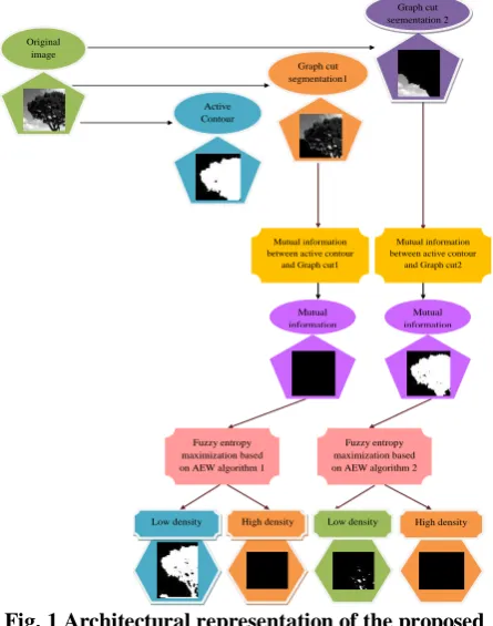
SEGMENTATION Proposed Architecture

As per the proposed method, an image I

 

x,y is subjected to active contour model, where a mask is deployed for segmenting the given image. By exploiting the mask, the optimal region could be segmented separately that is denoted byB

 

x,y . In addition, the original image I

 

x,y is given to graph cut scheme that split the image into two segments.

 

x y

C , _andD

 

x,y _{. The two divisions are further compared}

with active contour image B

 

x,y , and the mutual information of two images withB

 

x,y is taken , which is denoted as E

 

x,y andA

 

x,y . Moreover, FEM helps to separate the low intensity, and high intensity pixels of both

 

x y

E , _andA

 

x,y _{images. Accordingly, the low intensity}

images are indicated as E1

 

x,y _and A1

 

x,y _{, and high}

intesnity images are indicated as E2

 

x,y _andA2

 

x,y _{. As}

(4)

[image:4.595.63.286.54.337.2]

VARIABLE PARAMETRIC ERROR

Fig. 1 Architectural representation of the proposed image segmentation model

The fuzzy 2-partition entropy function of the adopted AEW-AGFES method is denoted by F . The variables

w v

u, , _{, together indicated by}_X_{that denotes the shape of} W_{membership function of fuzzy is provided as solution to} AEW scheme as shown by Fig. 2, where the objective is to maximize the entropyF_{as specified in Eq. (16).}

) (F Max

Objective ₍₁₆₎

Fig.2 Solution Encoding Proposed AEW model

The fuzzy entropy constraints u,v,w are offered to AEW model for optimization. In general, whales [22] have the ability to identify the location of prey and encircle them. This feature is mathematicaly indicated by Eq. (17) and Eq. (18), where, t refers to the present iteration, the position vector of whale is indicated byQ, position vector of prey is indicated by



Q _,_U_andQ

denotes the vector coefficient, ‘·’ denotes element-by-element multiplication and depicts the absolute value.

   

t Qt Q

U

E .  

(17)

 

t Q

 

t XE

Q 1    .

(18) It is essential to observe that



Q

has to be updated in the entire iterations with an improved solution. The vectors X

and U



are estimated as given by Eq. (19) and Eq. (20) in which the value of a



is linearly minimized from 2 to 0 for

further iterations and v



indicates a random vector, which lies among 0 and 1.

a v a X 2.

(19)

v

U2.₍₂₀₎

Exploitation Phase:

Shrinking encircling method: This phase is carried out by minimizing the value of a



in Eq. (18). In addition, note that the variation of X_{is minimized by}a_{, here}X_lies

between



a a



 

,

 _{in a random manner and}a_{is reduced from}

2 to 0 for more iterations.

Spiral updating location: The distance between the whales positioned at



Q,Y



and prey positioned at





 

Y

Q , _are

estimated in this process. A spiral model is included for identifying the location of prey and whale as given in Eq. (21)

in which E' Q (t) Q(t)

  



 

and it specifies the distance of th

i _{whale’s towards the prey, the constraint for relating the}

logarithmic spiral shape is shown by u, and h refers to an varying constraint that lies among [−1,1] and



0.5.

 

t 1 E.e .cos

 

2 h Q (t)

Q   uh  

 

 ₍₂₁₎

 

           _    pe if t Q h e E pe if E X t Q t Q uh ) ( 2 cos . '. . ) (

1  

   

(22) The final updated formula is based on Eq. (22) where pe denotes parametric error that lies among 0 and 1.

Exploration Phase:

Here, a randomly chosen searching agent is recognized instead of the most excellent search agent. Here, X 1



emphasizes the exploration process and permits the adopted system to perform a global search as given by Eq. (23) and Eq. (24), where Qrand



denotes a arbitrary whale, that is selected from the population existed.

Q Q U

E ._rand  

(23)

 

t Q XE

Q 1  _rand .

(24) The proposed AEW algorithm is enhanced by establishing a bounding factor, denoted by o as presented in Eq. (25), in which lb refers to the lower bound and ubdenotes the upper bound, and the maximum iteration is referred by Max(t) . Here, the distance indicated by D_{between the best position}

and current position is specified by Eq. (26).







/4





 





1/ ()



2



 ub lb ub lb t Max t

o ₍₂₅₎

position Best

position Current

D 

(26)

The count of higher Mutual information

between active contour and Graph cut1

Mutual information between active contour

and Graph cut2

Fuzzy entropy maximization based on AEW algorithm 1

Fuzzy entropy maximization based on AEW algorithm 2

Low density High density Low density High density Original image Active Contour model Graph cut segmentation1 12 Graph cut segmentation 2 Mutual information 1 Mutual information 2

(5)

solution constraints in D_{compared with}o_{is checked and}

is indicated byrs_{Depending on}rs_{, the vectors}X



and

U _{are approximated as shown in Eq. (27) and Eq.(28) by}

means of v1



and v2



denoted in Eq. (29) and Eq. (30), correspondingly.

a v a

X2.₁₍₂₇₎

2

. 2v U 

(28)



( )/ ( ) 0.01



1() 1 lengtho lengthr rand

v  s  



(29) v2



length(o)/length(rs)0.01



rand2()



(30)

The below Algorithm 1 depicts the pseudo code for the adopted AEW scheme.

Algorithm 1: AEW-AGFES algorithm Step1 _{Assign whale’s population}Q_i



i1,2,....,n



Step2 Find out fitness values of all exploring agents Step3

The most desired agent for search is



Q

Step4 While tis lower than total iterations For entire searching agents Step5 Determine oas per Eq. (25)

Step6 Compute distance D_{as per Eq. (26)}

Step7

Find v1



and v2



as per Eq. (29) and Eq. (30). Step8

Update a,Q,U,hand pe Step9 _{if 1} pe



Step10

if 2



X 1



Position of current search agent is updated as per Eq. (18)

Step11

else if 2



X 1



Choose a random search agent Qrand 

Update position of present search agent as per Eq. (24)

end if 2 Step12 else if 1 pe

Update position of present search agent as per Eq. (21)

end if 1 end for

Step13 Verify if any search agent exceeds the search space

Step14 Evaluate fitness value of search agent Step15

Update



Q _{if there is an enhanced solution}

Step16 tt1

end while return



Q

V. RESULTSANDDISCUSSIONS Experimental Set up

The proposed AEW-AGFES-based image segmentation model was implemented in MATLAB. The database Weizmann was used that was downloaded from “http://www.wisdom.weizmann.ac.il/~vision/Seg_Evaluatio

n_DB/”. It comprises of seven sets of images that consists animals, birds, nature, objects, transportation, and tree. In every set, few images were taken for this experiment, i.e., 12 images were considered for birds, 15 images were considered for animals, 26 images were considered for objects, 9 images were considered for transportation and 10 images were considered for tree. Here, algorithmic analysis was held by varying the values of from =0.25, =0.40, =0.55, =0.70 and =0.85 and performance measures like accuracy, sensitivity, specificity, and precision, FPR, FNR, NPV, FDR, F1-score, and MCC are analyzed. The segmentation output of adopted method is revealed in Fig. 3.

Image types

Original AEW-AGF

ES

Proposed segmented

images

Animal

Bird

Buildin g

Nature

Object

Transp ortation

Tree

(a) (b) (c)

Fig.3 Sample images for each dataset and its corresponding segmented output for (a) Original image (b) AEW-AGFES-based segmented image (c) proposed

segmented images

(6)

VARIABLE PARAMETRIC ERROR Algorithmic Analysis & RESULTS

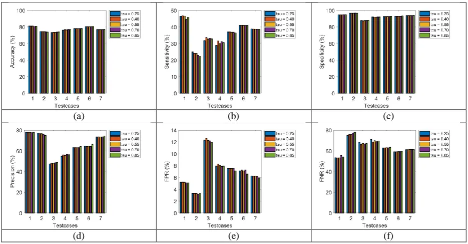
The algorithmic analysis of the suggested AEW-AGFES method for image segmentation is specified in Fig. 4. In Fig. 4(a), the accuracy of adopted model at 6th test case for

25 . 0





is 2.5% superior to



0.40, 2.5% superior to

55 . 0





, 2.5% superior to



0.70 and 2.5% superior to

85 . 0





.

From Fig. 4(b), the sensitivity of the implemented scheme at 1st test case for



0.40 is 2.17% superior to



0.85. Also, at 5th test case, the implemented scheme for



25 . 0





, 2.86% superior to



70 . 0





. In addition, at 8th test case, the presented system for



55 . 0





and 2.7% superior to



0.70.

From Fig. 4(c), the specificity of the implemented process at 4th test case for



0.25is 1.19% superior to



0.40, 1.19% better than



0.70 and 1.19% better than



0.85. Moreover, at 5th test case, the implemented scheme for



0.85 is 1.19% better than

25 . 0





, 1.19% better than



40 . 0





and 1.19% better than



0.70. In addition, at 6th test case, the presented system for



0.25,



0.55,



0.40 and



0.70. Also at 7th test case, the presented system for



0.25,



0.55,



0.40 and



0.70.

From Fig. 4(d), at 1st test case, the implemented scheme for



0.85 is 1.29%better than



55 . 0





, 1.29% better than



70 . 0





. In addition, on considering 7th test case, the implemented scheme for



25 . 0





, 2.78% better than



40 . 0





0.70. Also, FPR of the suggested model can be attained from

Fig. 4(e), where the adopted model at 1st test case, for

70 . 0





is 9.61% superior to



55 . 0





, 9.61% superior to



70 . 0





. Moreover, at 2nd test case, the proposed scheme for

70 . 0





is 3.23% superior to



55 . 0





, 3.23% superior to



70 . 0





.

Accordingly, from Fig. 4(f), the adopted scheme on considering 7th test case, for



25 . 0





, 1.54% better than



40 . 0





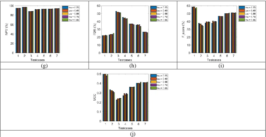
0.70.

From Fig. 4(g), the NPV of the adopted scheme at 5th test case and 6th test case for



25 . 0





, 1.09% superior to



40 . 0





0.70.

In addition, the FDR, F1-score and MCC of the adopted model for varying values of  from  =0.25,  =0.40,  =0.55,  =0.70 and  =0.85 are portrayed by Fig. 4(h), Fig. 4(i) and Fig. 4(j).

(a) (b) (c)

[image:6.595.64.532.447.691.2]

(7)

(g) (h) (i)

[image:7.595.65.531.49.290.2]

(j)

Fig. 4. Performance analysis of the proposed model in terms of (a) Accuracy (b) Sensitivity (c) Specificity (d) Precision (e) FPR (f) FNR (g) NPV (h) FDR (i) F1 core (j) MCC

Overall Performance Analysis

The performance analysis of the implemented image segmentation scheme when evaluated by varying the values of  from



0.25 ,



0.40 ,



0.55,



0.70 and

85 . 0





for seven test cases is specified from Table I to Table VII, respectively.

Accordingly, from Table I, for test case 1, the accuracy of the proposed scheme for



25 . 0





, 3.69% better than



70 . 0





0.85. In the same way, the sensitivity of the implemented scheme for



0.85. From Table II, for test case 2, the specificity of the presented design for



0.55 and

0.92% better than



0.85 . Also, the precision of the adopted scheme for



0.25is 0.65% superior to



0.85.

From Table III, for test case 3, the FPR of the proposed scheme for



0.70. In addition, for test case 3, the FPR of the proposed scheme for



25 . 0





, 1.22% superior to



70 . 0





0.85. Similarly, the same analysis is repeated for all test cases, and the proposed performance efficacy has been proven.

[image:7.595.150.449.567.711.2]

TABLE 1. ALGORITHMIC ANALYSIS ON TEST CASE 1

Measures



0.25



0.40



0.55



0.70



0.85

Accuracy 0.81145 0.81193 0.81163 0.80657 0.81021

Sensitivity 0.46536 0.46757 0.46589 0.44527 0.45891 Specificity 0.94792 0.94772 0.94796 0.94904 0.94874

Precision 0.77894 0.7791 0.77925 0.77504 0.77925

FPR 0.052078 0.052276 0.052043 0.050963 0.051265

FNR 0.53464 0.53243 0.53411 0.55473 0.54109

NPV 0.94792 0.94772 0.94796 0.94904 0.94874

FDR 0.22106 0.2209 0.22075 0.22496 0.22075

F1-score 0.58264 0.58441 0.58314 0.56559 0.57764

MCC 0.49672 0.49824 0.49725 0.4814 0.49276

(8)

Measures



0.25



0.40



0.55



0.70



0.85

Accuracy 0.74557 0.74311 0.74311 0.73997 0.73705

Precision 0.77037 0.76543 0.76543 0.76205 0.75071

FPR 0.033213 0.032984 0.032984 0.031827 0.032755

FNR 0.75025 0.75876 0.75876 0.77154 0.77891

NPV 0.96679 0.96702 0.96702 0.96817 0.96724

FDR 0.22963 0.23457 0.23457 0.23795 0.24929

F1-score 0.37721 0.36686 0.36686 0.35154 0.34158

MCC 0.33335 0.32466 0.32466 0.31349 0.30266

Measures



₀_.₂₅



₀_.₄₀



₀_.₅₅



₀_.₇₀



₀_.₈₅

Accuracy _0.7331 _0.73555 _0.73582 _0.73758 _0.73837

Precision _0.47251 _0.48035 _0.48062 _0.48568 _0.4877

FPR 0.12303 0.12592 0.12272 0.12203 0.11942

FNR _0.68201 _0.66416 _0.67233 _0.66752 _0.67198

NPV _0.87697 _0.87408 _0.87728 _0.87797 _0.88058

FDR 0.52749 0.51965 0.51938 0.51432 0.5123

F1-score _0.38015 _0.3953 _0.38967 _0.39473 _0.39223

MCC _0.22523 _0.23891 _0.23556 _0.2415 _0.24105

Measures



0.25



0.40



0.55



0.70



0.85

Accuracy 0.76291 0.76725 0.76508 0.7687 0.76702

Precision 0.54897 0.56114 0.55551 0.5682 0.56265

FPR 0.079147 0.082436 0.080398 0.078823 0.079141

FNR 0.71097 0.68375 0.69853 0.6888 0.69453

NPV 0.92085 0.91756 0.9196 0.92118 0.92086

FDR 0.45103 0.43886 0.44449 0.4318 0.43735

F1-score 0.37869 0.40452 0.39084 0.40215 0.39597

MCC 0.26882 0.29101 0.27955 0.29271 0.28614

Measures



0.25



0.40



0.55



0.70



0.85

Accuracy 0.78037 0.78037 0.78002 0.78022 0.78201

Precision 0.63315 0.63325 0.63235 0.63311 0.64254

FPR 0.075222 0.075139 0.075196 0.074978 0.071246

FNR 0.63057 0.63081 0.63196 0.63183 0.63557

NPV 0.92478 0.92486 0.9248 0.92502 0.92875

FDR 0.36685 0.36675 0.36765 0.36689 0.35746

F1-score 0.4666 0.46644 0.46528 0.46559 0.46508

MCC 0.35973 0.35966 0.35843 0.35898 0.36269

(9)

Measures



0.25



0.40



0.55



0.70



0.85

Accuracy 0.80392 0.80298 0.80355 0.80265 0.80777

Precision 0.64586 0.64198 0.64504 0.6413 0.66345

FPR 0.071315 0.07251 0.071294 0.072439 0.065707

FNR 0.58969 0.58981 0.59128 0.59143 0.59136

NPV 0.92869 0.92749 0.92871 0.92756 0.93429

FDR 0.35414 0.35802 0.35496 0.3587 0.33655

F1-score 0.50182 0.50055 0.50038 0.49914 0.50576

MCC 0.40268 0.40017 0.40123 0.39881 0.41256

Measures



0.25



0.40



0.55



0.70



0.85

Accuracy 0.76798 0.76798 0.76762 0.76766 0.76996

Precision 0.73522 0.7354 0.73469 0.73524 0.74486

FPR 0.062411 0.062322 0.062384 0.062144 0.059262

FNR 0.61187 0.61207 0.61312 0.6135 0.61252

NPV 0.93759 0.93768 0.93762 0.93786 0.94074

FDR 0.26478 0.2646 0.26531 0.26476 0.25514

F1-score 0.50805 0.50792 0.50686 0.50666 0.50977

MCC 0.40741 0.40739 0.40629 0.40639 0.41298

CONCLUSION

This paper has presented an enhanced image segmentation technique using Active Contour, and Graph cut schemes. Here, the high-intensity and low-intensity pixels of the segmented images were clustered by FEM model, in which the maximization problem was solved by means of proposed AEW algorithm. By the exploitation of this adopted scheme, the segmentation accuracy was found to have improved in a better way. Moreover, algorithmic analysis was performed for the proposed system by varying the values of from  =0.25,  =0.40,  =0.55,  =0.70 and  =0.85 in terms of relevant performance measures for 7 test cases. From the analysis, the accuracy of proposed model at 6th test case for

25 . 0





was 2.5% superior to



55 . 0





, 2.5% superior to



85 . 0





. Thus the betterment of the presented scheme has been substantiated effectively.

REFERENCES

1. S. K. Choy, Kevin Yuen, Carisa Yu, “Fuzzy

bit-plane-dependence image segmentation”, Signal Processing, vol. 154, pp. 30-44, January 2019.

2. Li Guo, Long Chen, C. L. Philip Chen, Jin Zhou, “Integrating

guided filter into fuzzy clustering for noisy image segmentation”, Digital Signal Processing, vol. 83, pp. 235-248, December 2018.

3. PengGu, Won-MeanLee, Marilyn A.Roubidoux, JieYuan,

XuedingWang and Paul L.Carson, "Automated 3D ultrasound image segmentation to aid breast cancer image interpretation", Ultrasonics", vol. 65, pp. 51-58, 2016.

4. Zexuan Ji, Yubo Huang, Yong Xia, Yuhui Zheng, “A robust

modified Gaussian mixture model with rough set for image segmentation”, Neurocomputing, vol. 266, pp. 550-565, 29 November 2017.

5. Andrea Pennisi, Domenico D. Bloisi, Daniele Nardi, Anna Rita

Giampetruzzi, Antonio Facchiano, “Skin lesion image

segmentation using Delaunay Triangulation for melanoma

detection”, Computerized Medical Imaging and Graphics, vol. 52, pp. 89-103, September 2016.

6. Yiping Duan, Fang Liu, Licheng Jiao, Peng Zhao, Lu Zhang, “

SAR Image segmentation based on convolution-wavelet neural network and Markov random field”, Pattern Recognition, vol. 64, pp. 255-267, April 2017.

7. M. Guijarro, I. Riomoros, G. Pajares, P. Zitinski, “ Discrete

wavelets transform for improving greenness image segmentation in agricultural images”, Computers and Electronics in Agriculture, vol.118, pp 396-407, October 2015.

8. Jianning Chi, Mark Eramian, “Enhancing textural differences

using wavelet-based texture characteristics morphological component analysis: A pre-processing method for improving

image segmentation”, Computer Vision and Image

Understanding, vol.158, pp. 49-61, May 2017.

9. Zhang Yong, Yuan Jiazheng, Liu Hongzhe, Li Qing, “Grab-Cut

image segmentation algorithm based on structure tensor”, The Journal of China Universities of Posts and Telecommunications, vol. 24, no. 2, pp. 38-47, April 2017

10. Yafeng Li, Xiangchu Feng, “A multi-scale image segmentation

method”, Pattern Recognition, vol.52, pp. 332-345, April 2016.

11. Yongsheng Pan, Yong Xia, Tao Zhou, Michael Fulham, ”Cell

image segmentation using bacterial foraging optimization”, Applied Soft Computing, vol. 58, pp.770-782, September 2017.

12. Weiwei Wang, Cuiling Wu, “Image segmentation by correlation

adaptive weighted regression”, Neuro computing , 29 June 2017.

13. Iasonas Kokkinos; Petros Maragos, “Synergy between Object

Recognition and Image Segmentation Using the

Expectation-Maximization Algorithm”, IEEE Journals & Magazines, vol.31, no.08, pp.1486 - 1501, 2009.

14. Yousun Kang; Koichiro Yamaguchi; Takashi Naito; Yoshiki

Ninomiya,”Multiband Image Segmentation and Object Recognition for Understanding Road Scenes”, IEEE Journals & Magazines, vol.12, no.04, pp.1423 - 1433, 2011

15. Fuzhuan Wu, Bingxin Wu,”Design and Realization of Fuzzy

Control System for Textile Mill's Air-Conditioning Based on MSP430”, IEEE Conference Publications, pp.1 - 4, 2010.

16. Gang Zheng; Yuanlu Li; Huinan Wang, “A New Multi-phase

(10)

17. Zhuowen Tu; Song-Chun Zhu, “Image segmentation by

data-driven Markov chain Monte Carlo”, IEEE Journals & Magazines , vol.24, no.05, pp.657 - 673, 2002.

18. Kyumok Kim; Seung-Won Jung,“ Interactive Image

Segmentation using Semi-transparent Wearable Glasses”, IEEE Transactions on Multimedia, Vol. PP, no. 99, pp. 1 – 1, 2017.

19. Changjae Oh, Bumsub Ham, Kwanghoon Sohn, “Robust

interactive image segmentation using structure-aware labelling”, Expert Systems with Applications, vol. 79, pp. 90-100, 15 August 2017.

20. Hiren K. Mewada, Amit V. Patel, Keyur K. Mahant, “Concurrent

design of active contour for image segmentation using Zynq ZC702”, Computers & Electrical Engineering, vol. 72, pp. 631-643, November 2018.

21. Guowei Gao, Chenglin Wen, Huibin Wang, “Fast and robust

image segmentation with active contours and Student's-t mixture model”, Pattern Recognition, vol. 63, pp. 71-86, March 2017.

22. Seyedali Mirjalili, Andrew Lewis, “The Whale Optimization

Algorithm”, Advances in Engineering Software, vol. 95, pp. 51-67, May 2016. ultrasound volumes

23. M. Jogendra Kumar, and Dr. G.V.S. Raj Kumar, "Hybrid Image

Segmentation Model based on Active Contour and Graph cut with Fuzzy Entropy Maximization", International Journal of Applied Engineering Research, vol.12, no.23, pp. 13623-13637, 2017.

24. G.V.S. Raj Kumar and M. Jogendra Kumar, "A Refined Image

Segmentation Model Under Adaptiveness on Whale