An empirical zenith wet delay correction model using piecewise height functions

https://doi.org/10.5194/angeo-36-1507-2018 © Author(s) 2018. This work is distributed under the Creative Commons Attribution 4.0 License.

An empirical zenith wet delay correction model using

piecewise height functions

YiBin Yao1,2,3and YuFeng Hu1,4

1_{School of Geodesy and Geomatics, Wuhan University, 129 Luoyu Road, Wuhan 430079, China} 2_{Key Laboratory of Geospace Environment and Geodesy, Ministry of Education, Wuhan University,} 129 Luoyu Road, Wuhan 430079, China

3_{Collaborative Innovation Center for Geospatial Technology, 129 Luoyu Road, Wuhan 430079, China} 4_{College of Geology Engineering and Geomatics, Chang’an University, Xi’an 710054, Shanxi, China} Correspondence:YuFeng Hu ([email protected])

Received: 22 May 2018 – Discussion started: 28 May 2018

Revised: 4 September 2018 – Accepted: 18 October 2018 – Published: 6 November 2018

Abstract.Tropospheric delay is an important error source in space geodetic techniques. The temporal and spatial varia-tions of the zenith wet delay (ZWD) are very large and thus limit the accuracy of tropospheric delay modelling. Thus, it is worthwhile undertaking research aimed at constructing a precise ZWD model. Based on the analysis of vertical varia-tions of ZWD, we divided the troposphere into three height intervals (below 2 km, 2 to 5 km, and 5 to 10 km) and deter-mined the fitting functions for the ZWD within these height intervals. The global empirical ZWD model HZWD, which considers the periodic variations of ZWD with a spatial reso-lution of 5◦_×5◦_{, is established using the ECMWF ZWD} pro-files from 2001 to 2010. Validated by the ECMWF ZWD data in 2015, the precision of the ZWD estimation in the HZWD model over the three height intervals are improved by 1.4, 0.9, and 1.2 mm, respectively, compared to that of the cur-rently best GPT2w model (23.8, 13.1, and 2.6 mm). The test results from ZWD data from 318 radiosonde stations show that the root mean square error (RMSE) in the HZWD model over the three height intervals was reduced by 2 % (0.6 mm), 5 % (0.9 mm), and 33 % (1.7 mm), respectively, compared to the GPT2w model (30.1, 15.8, and 3.5 mm) over the three height intervals. In addition, the spatial and temporal stabil-ities of the HZWD model are higher than those of GPT2w and UNB3m.

1 Introduction

The radio waves experience propagation delays when pass-ing through the neutral atmosphere (primarily the tropo-sphere), which are known as the tropospheric delays. The tropospheric delay is one of the main error sources in space geodetic techniques. In the processing of the space geode-tic data, the tropospheric delay along the propagation path is generally expressed as the product of zenith tropospheric delay (ZTD) and mapping function (MF). The ZTD is di-vided into a zenith hydrostatic delay (ZHD) and a zenith wet delay (ZWD) (Davis et al., 1985), and the ZHD can be ac-curately determined using pressure observations. Unlike the ZHD, the ZWD is difficult to calculate accurately due to the high spatio-temporal variation in water vapour. Its spatial dis-tribution is characterized with a near-zonal dependency, with values varying from about 2 cm at high latitudes to about 35 cm near the Equator (Fernandes et al., 2013). The tempo-ral variation pattern of ZWD is mainly characterized by the seasonal variability, including annual and semi-annual com-ponents (Jin et al., 2007; Nilsson et al., 2008). The high vari-abilities in ZWD make it the main factor influencing tropo-spheric delay correction.

mod-els, such as total column water vapour (TCWV) and tem-perature. While Stum et al. (2011) proposed a model that only uses TCWV. These models provide similar results to the study of Davis et al. (1985) (that uses 3-D parameters) but only at the level of the model orography to which the meteorological parameters refer to. As this orography may depart significantly from the actual surface, and the vertical variation of the ZWD is not well known, at a different el-evation they possess errors associated with the uncertainty in the modelling of the ZWD height variation (Fernandes et al., 2013, 2014; Vieira et al., 2018). The traditional Saasta-moinen model (1972) and Hopfield model (1971) approxi-mate the ZWD with surface observations as temperature and water vapour pressure observations. Without the information about the vertical distribution of water vapour, the stability and reliability of their ZWD estimates are poor. Moreover, both models are highly dependent on meteorological data. The aforementioned models have the limitations of applica-tion in wide area augmentaapplica-tion and real-time navigaapplica-tion and positioning. Therefore, the empirical climatological models were proposed as required practical conditions. The RTCA-MOPS (2016), designed by the US Wide Area Augmentation System (Collins et al., 1996), estimates ZWD by using the latitude band parameters table. The modified RTCA-MOPS model – called UNB3m (Leandro, 2006) – uses relative hu-midity as a parameter instead of the water vapour pressure to calculate the ZWD, effectively improving the precision of ZWD estimation to 5.5 cm (Möller et al., 2014), but the model deviation is increased when the height exceeds 2 km (Leandro, 2006). The TropGrid model (Krueger et al., 2004, 2005) provides the meteorological parameters needed to cal-culate tropospheric delay in the form of a 1◦_×1◦_{grid. The} improved TropGrid2 model (Schüler, 2014) enhances the ef-ficiency of ZWD calculation by directly modelling ZWD with the exponential function. Based on the GPT2 model (Lagler et al., 2013), the GPT2w model (Böhm et al., 2015) adds weighted mean temperature and a vapour pressure de-crease factor realised as a global grid to estimate ZWD by using the Askne and Nordius formula (Askne and Nordius, 1987). The GPT2w model has the best precision of ZWD es-timation (3.6 cm) compared to other commonly used models (Möller et al., 2014).

The water vapour changes rapidly with respect to height, and the trends in water vapour at different heights vary, so the wet delay with direct relation to water vapour has complex spatio-temporal variations in the vertical direction. Kouba (2008) proposed an empirical exponential model to account for the height dependency of ZWD, but it will only be applicable within the height below 1000 m. The aforemen-tioned empirical models are all based on a fixed height (av-erage sea level or surface height) and use only a single de-crease factor to describe the variation of water vapour or wet delay with respect to height, which makes it difficult to al-low for the vertical distribution differences in water vapour (or wet delay) in the upper troposphere. In the course of

air-Figure 1.Water vapour pressure profile(a)and ZWD profile(b)at a grid point (0◦N, 0◦E) at 12:00 UTC on 1 January 2010.

craft dynamic navigation and positioning, the zenith delay error will result in twice as many errors in the station height estimate (Böhm and Schuh, 2013). Thus, it is necessary to correct the wet delay at different heights, which is clearly difficult for the aforementioned models. Based on the anal-ysis of the characteristics of the ZWD profile, an empirical ZWD model, named HZWD, is established based on three functions applicable within corresponding height intervals, and the model precision is verified by European Centre for Medium-Range Weather Forecast (ECMWF) reanalysis data as well as radiosonde data.

2 Vertical variations of ZWD

ZWD is defined as the integral of the wet refractivity along the vertical profile above the station.

ZWD=10−6 ∞ Z

H

Nwdh=10−6 ∞ Z

H

(k0₂e T +k3

e

T2)dh (1)

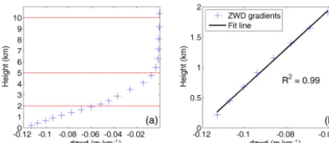
Figure 2. ZWD vertical gradients profile (a)and linear fit with height below 2 km(b) at a grid point (0◦N, 0◦E) at 12:00 UTC on 1 January 2010.

a suitable fitting function capable of describing the changes in ZWD with respect to height.

ERA-Interim can provide data at 00:00, 06:00, 12:00, and 18:00 UTC daily with a spatial resolution of not more than 0.75◦×0.75◦and 37 pressure levels (Dee et al., 2011). The highest level data come from a height of approximately 50 km, covering almost the entire troposphere and strato-sphere. We used the temperature, the geopotential height, and the specific humidity provided by the ERA-Interim pressure level data, and the discretised form of Eq. (1), to calculate the ZWD for each level height (Böhm and Schuh, 2013). 

    

    

ei =qi×Pi/(0.622+0.378×qi)

Nwi=k 0 2

ei

Ti +k3

ei

T_i2

ZWD=10−6 36 P

i

Nwi+Nwi+1

2 ·(hi+1−hi)

(2)

In Eq. (2),qis the specific humidity in grammes per gramme (g g−1), P is the pressure in hPa, k₂0 andk3 are empirical constants same as Eq. (1), andh is the geopotential height in metres. From Eq. (2), we can see that the ZWD at a spe-cific level height is the sum of the ZWD portions in all lay-ers above the specific level height. Figure 1 shows the wa-ter vapour pressure and ZWD profiles at a grid point (0◦N, 0◦E) at 12:00 UTC on 1 January 2010. From Fig. 1, it can be seen that the downward trend in the water vapour pres-sure varies significantly with height, and the decrease factor is different across different height intervals. The changes in ZWD with respect to height are similar to that of the water vapour pressure with respect to height: the decay is fastest up to a few kilometres height and slows down with increasing height; the ZWD values are close to zero after 10 km. Zhao et al. (2014) showed that about 50 % of the water vapour con-tent is concentrated within 1.5 km of the surface and less than 10 % of the water vapour content remains above 5 km, lead-ing to different ZWD decay rates within different height in-tervals. These results are basically consistent with our experi-ment results. Further, the derivative of the ZWD with respect to height (i.e. ZWD vertical gradient) is analysed to better understand the characteristic of the ZWD vertical

distribu-Figure 3.ZWD gradients profiles at grid points in different latitude bands (12:00 UTC, 1 January 2010).

tions. Figure 2a shows the variation of ZWD vertical gradi-ents with respect to height at the same grid point to Fig. 1. From Fig. 2a, it can be seen that the trends in ZWD verti-cal gradients at different height intervals are clearly different. Specifically, the linear fit of the ZWD gradients with height below 2 km shows a great agreement with anR2value of 0.99 (Fig. 2b). Thus we can come to a conclusion: ZWD gradients roughly change linearly below 2 km. From 2 to 5 km, and 5 to 10 km, the ZWD gradients vary non-linearly.

Figure 4.ZWD gradients profiles at grid points in different latitude bands (12:00 UTC, 1 July 2010).

Table 1. Fitting RMSE of piecewise height functions, single quadratic polynomial function, and single exponential function (unit: mm).

< 2 km 2 km to 5 km 5 to 10 km Piecewise height 0.2 1.0 0.2 functions

Quadratic 5.9 3.8 6.5 polynomial

Exponential 2.3 2.2 1.0

fitting with respect to height, TropGrid2 and GPT2w use ex-ponential functions, while some scholars have also used a polynomial to describe the tropospheric delay with respect to height (Song et al., 2011). We used both polynomial and ex-ponential functions to fit the variation trend of the ZWD with respect to height in the three selected intervals, respectively. The results showed that the quadratic polynomial used under 2 km and the exponential functions between 2 and 5 km and between 5 and 10 km gave the best fits. The combination of the quadratic polynomial and exponential functions for dif-ferent height intervals are termed piecewise height functions. Table 1 summarises the global fitting statistics of different fit functions, demonstrating the superiority of piecewise height functions to the single polynomial function and single expo-nential function used for the whole troposphere.

Figure 5.Decadal time series and cycle fitting results of function coefficientsz1(a),z2 (b), andz3(c)at a grid point (0◦N, 0◦E)

from 2001 to 2010.

3 The HZWD model

From the above analysis of ZWD vertical variation and fit-ting, the piecewise height functions of the proposed HZWD model are:

ZWD(B, L, H )=            

          

z1+a1·H+a2·H2 H <2000 m z2·exp{β2·(H−2000)}

2000 m≤H <5000 m z3·exp{β3·(H−5000)}

5000 m≤H≤10 000 m 0

H >10 000 m

(3)

of 0, 2, and 5 km, respectively. We used the monthly mean profiles of ERA-Interim pressure levels from 2001 to 2010 with a horizontal resolution of 5◦_×5◦_{for ZWD modelling.} The ZWD profiles calculated for each grid point are fitted by Eq. (3) to obtain the time series of the corresponding func-tion coefficients: z1,a1,a2,z2,β2,z3, and β3. It is worth noting that the ERA-Interim-derived ZWD data indicate that the averaged ZWD values at the three height intervals (i.e. below 2, 2 to 5 km, and 5 to 10 km) are 0.126, 0.0489, and 0.0111 m, respectively. Jin et al. (2007) found that the tropo-spheric delay has notable seasonal variations, mainly on an-nual and semi-anan-nual cycles. Song et al. (2011) and Zhao et al. (2014) considered the temporal features of function coeffi-cients in their troposphere models. We used the 10-year time series of those coefficients obtained to analyse their tempo-ral variations. Figure 5 shows the time series and cycle fit-ting results of the function coefficientsz1,z2, andz3at grid point (0◦_{N, 0}◦_{E). Figure 5 shows that the time series of the} function coefficientsz1,z2, andz3have a significant charac-teristic annual cycle, and the semi-annual cycle is small but nevertheless evident.

Therefore, taking the annual and semi-annual cycles into consideration, we used Eq. (4) to fit the function coefficients derived from Eq. (3) to temporal parameters for each grid point (Böhm et al., 2015).

r(t )=c0+c1cos

_doy

365.252π

+b1sin

_doy

365.252π

+c2cos

_doy

365.254π

+b2sin

_doy

365.254π

(4) In Eq. (4),c0is the annual mean,c1andb1are the annual cy-cle parameters,c2andb2are the semi-annual cycle parame-ters, and doy is the day of the year. The fittings show that the annual means and annual and semi-annual amplitudes ofz1, z2, andz3are distinct. For instance, the cycle fitting results at a grid (0◦N, 0◦E) (Fig. 5) indicate that the temporal pa-rameters (i.e.c0,c1,b1,c2, andb2) ofz1are 0.2911, 0.0237, 0.0312, −0.0006, and−0.0227 m, respectively; the tempo-ral parameters ofz2are 0.1215, 0.0118, 0.0203, 0.0004, and

−0.0146 m, respectively; the temporal parameters ofz3 are 0.0255, 0.00031, 0.0070,−0.0019, and−0.0044 m, respec-tively. It should be noted that the fitting results of coefficients a2,β2, andβ3 show that all their annual means and annual and semi-annual amplitudes are small. However, below 2 km, the lack of cycle terms ina2would cause centimetre-level er-rors in the ZWD estimates, so these terms have been retained. Forβ2andβ3, ZWD itself is small at heights above 2 km, so the annual mean suffices for a desirable ZWD estimate. The experiment reveals that the loss of accuracy due to the lack of annual and semi-annual terms inβ2andβ3for the ZWD esti-mates is less than 0.1 mm. Therefore, only the annual means are retained for these two coefficients.

Figure 6 shows the global distributions of annual means of model coefficientsz1,z2, andz3. From Fig. 6 we can see

Figure 6.Global distributions of annual means of HZWD model coefficientsz1(a),z2(b), andz3(c).

that the extremum of ZWD annual means at 0 m height oc-cur near the Equator and the maximum exceeds 0.36 m. The ZWD annual means decrease with increasing latitude. The distributions of ZWD annual means at 2 and 5 km heights are similar to that at 0 m, but the areas with the large val-ues near the Equator decrease in extent and the ZWD distri-butions tend to be uniform, indicating that the water vapour content near the Equator is greater than that in other regions, and the ZWD value is also larger in low-altitude regions. As the height increases, the difference in water vapour content or ZWD between the Equator and other areas begins to de-crease, but remains significant. Overall, there are some dif-ferences in the ZWD distribution at different heights, and it is necessary to model the spatio-temporal variations of ZWD at different heights.

coeffi-cients,z1,z2,z3,a1, anda2are further expressed by Eq. (4) with five temporal parameters, respectively. Therefore, there are 27 parameters for each grid point and total 68 094 param-eters for the HZWD model. As a comparison, the GPT2w model has a number of 77 760 parameters, which is 14 % more than that of the HZWD model. It is worth noting that the UNB3m model only has 50 parameters due to its coarse spatio-temporal resolution. When the HZWD model is ap-plied, the four grid points surrounding the station are deter-mined according to the horizontal position (latitude and lon-gitude) of the station, and then the model coefficients of the corresponding height intervals at the four selected points are calculated according to Eq. (4). The ZWD of the four grid points are extrapolated to the station height by using Eq. (3), and finally the ZWD at the station location is obtained by using bilinear interpolation. The HZWD model only needs time, latitude, longitude, and height as input parameters. It can calculate ZWD without meteorological data and can pro-vide wet delay correction products for navigation and posi-tioning at different heights.

4 Validation and analysis of the HZWD model

To test the precision of the HZWD model and analyse the model correction performance compared to other tro-posphere models, we used the ERA-Interim pressure level data and radiosonde data from the year 2015 as external data sources and compared the results with the commonly used models UNB3m and GPT2w. The parameters used for the validation are bias and root mean square error (RMSE), ex-pressed as follows.

Bias=1

n

n X

i=1

(ZWDM_i −ZWD0_i) (5)

RMSE= v u u t 1 n n X

i=1

(ZWDM_i −ZWD0_i)2 (6)

In Eqs. (5) and (6), ZWDM_i is the value estimated by the HZWD model developed in this study and ZWD0_i is the ref-erence value.

For the UNB3m model, the ZWD at mean sea level (m.s.l.) is first calculated, then a vertical correction is applied to transform the ZWD to the target height. The formulae are as follows (Leandro et al., 2006):

        

ZWD0=10−6

(Tmk₂0+k3)Rd gm(λ+1)−γ Rd

·e0

T0 ,

ZWD=ZWD0

1−γ H

T0 (λ

+1)g γ R_d −1

,

(7)

wheree0,T0, and ZWD0are the water vapour pressure, tem-perature, and ZWD at MSL, respectively;Rdis the specific gas constant for dry air (278.054 J kg−1K−1);γ andλ are

Table 2.Error statistics for the three models compared to the 2015 ECMWF data (unit: mm).

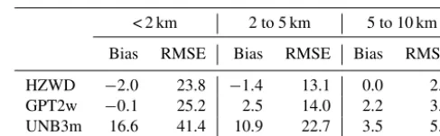
< 2 km 2 to 5 km 5 to 10 km Bias RMSE Bias RMSE Bias RMSE HZWD −2.0 23.8 −1.4 13.1 0.0 2.6 GPT2w −0.1 25.2 2.5 14.0 2.2 3.8 UNB3m 16.6 41.4 10.9 22.7 3.5 5.8

the temperature lapse rate and water vapour decrease factor, respectively;gmis the gravity acceleration at the mass centre of the vertical column of the atmosphere and can be com-puted with geodetic latitudeϕand heighthby

gm=9.7841−0.00266 cos 2ϕ−0.28·10−6h; (8) andTmis the weighted mean temperature computed by

Tm=T0

1− γ Rd

gm(λ+1)

. (9)

For the GPT2w model, the modelled meteorological param-eters at the four grid points surrounding the target location are extrapolated vertically to the desired height, and then the Askne and Nordius formula (10) is used to calculate the wet delays at those base points: finally the wet delays are inter-polated to the observation site in horizontal direction to get the target ZWD.

ZWD=10−6·(k0₂+ k3

Tm)· Rde

(λ+1)gm (10) In GPT2w model, Tm is an empirical parameter modelled with seasonal components andgmis simplified to a constant (9.80665 m s−2). It should be noted that the GPT2w model provides both 1◦×1◦and 5◦×5◦resolution versions. Since the horizontal resolution of the HZWD model is 5◦×5◦, we used the GPT2w model with the same resolution for valida-tion.

4.1 Validation with ECMWF data

Modelling of the HZWD model is based on the monthly mean profiles of ERA-Interim pressure level data from 2001 to 2010, while we used the ERA-Interim pressure level data with the full time resolution of 6 h in 2015 for the model vali-dation. This is to validate the model performance on the daily scale. Regarding the ZWD profiles calculated from these data as reference values, we calculated the global annual aver-age bias and RMSE of the ZWD for three models (HZWD, GPT2w, and UNB3m) within the three height intervals: be-low 2 km, 2 to 5 km, and 5 to 10 km (Table 2).

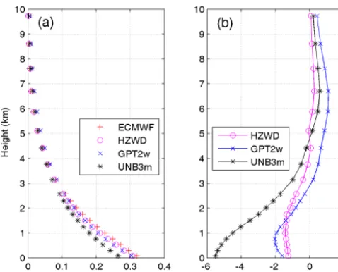
Figure 7.The ZWD profiles(a)of ECMWF and the three models (HZWD, GPT2w, and UNB3m) and corresponding biases(b)at a grid point (0◦N, 20◦E) at 12:00 UTC on 1 January 2015.

the GPT2w model, and the UNB3m model has the worst per-formance. The annual average biases of the HZWD model are lower than that of the GPT2w model and the UNB3m model, except below 2 km. Compared with the RMSEs in the GPT2w model, those of the HZWD model are decreased by 1.4, 0.9, and 1.2 mm within the three height intervals, cor-responding to improvements of about 6 %, 6 %, and 32 %, respectively. The improvements of the HZWD model over GPT2w model will result in precision improvements of 2.8, 1.8, and 2.4 mm respectively in height estimates in real-time aircraft positioning. The correction performance improve-ment from 5 to 10 km height is particularly evident. Figure 7a shows the ECMWF ZWD profile and the ZWD profiles of the three models at 12:00 UTC on 1 January 2015 at a represen-tative grid point (0◦N, 20◦E). More clearly, Fig. 7b shows the differences between the ZWD profiles of the three mod-els and ECMWF ZWD profile at different heights. It can be seen that HZWD is the most stable model, showing the best agreement with the ECMWF ZWD data, which is superior to both the GPT2w and the UNB3m models.

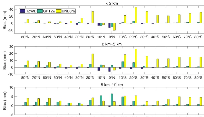
The variation of the troposphere has a strong correlation with latitude. To analyse the correction performances of the three models in different regions around the world, we calcu-lated the three models’ errors in different latitude bands (10◦ intervals). Figures 8 and 9 show the correction performances at different latitudes. It can be seen from Fig. 8 that the bias of the UNB3m model is basically positive in the three height intervals, indicating that its ZWD estimates are relatively large compared to the ECMWF data. Moreover, the bias in the Southern Hemisphere is significantly larger than that in the Northern Hemisphere, indicating systematic deviations in the Southern Hemisphere. Both the GPT2w model and the HZWD model have large biases in the low latitudes. The

bi-Table 3.Error statistics for the three models validated by 2015 ra-diosonde data (unit: mm).

< 2 km 2 to 5 km 5 to 10 km Bias RMSE Bias RMSE Bias RMSE HZWD −3.6 30.1 −2.0 15.8 0.1 3.5 GPT2w −3.2 30.7 3.5 16.7 3.3 5.2 UNB3m 5.9 46.0 6.2 23.1 2.6 5.7

ases of the GPT2w model are positive from 2 to 5 km and 5 to 10 km height, indicating that the ZWD is overestimated by the GPT2w model with increasing height. For the HZWD model, the bias in each latitude band is relatively small with few exceptions, resulting in a global average bias close to zero (see Table 2).

Figure 9 shows the RMSEs of the three models. It can be seen from Fig. 9 that the precision of the HZWD model is significantly better than that of the UNB3m model across the three height intervals and all latitude bands, which is better than the GPT2w model in general. The precision of the three models declines with decreasing latitude, because the active change in water vapour in these areas limits the precision of the model. Corresponding to Fig. 8, the errors in UNB3m are asymmetric: the main reason for this is that the meteorolog-ical parameters of UNB3m are interpolated from the coarse look-up table with a latitude interval of 15◦, and UNB3m does not consider the longitudinal variations of any meteo-rological elements. It should be pointed out that the UNB3m model is based on the simple symmetric assumption of the Northern and Southern Hemispheres, and its modelling data source only comes from the atmospheric data collected over North America, which leads to poor precision in the Southern Hemisphere, especially in the high latitudes thereof.

Figure 8.Bias comparisons between the three models (HZWD, GPT2w, and UNB3m) in different latitude bands over the year 2015.

Figure 9.RMSE comparisons between the three models (HZWD, GPT2w, and UNB3m) in different latitude bands over the year 2015.

4.2 Validation with radiosonde data

A radiosonde is used in a sounding technique that regularly releases balloons to collect atmospheric meteorological data at different heights: it can obtain profiles of various meteo-rological data with high accuracy. At present, the Integrated Global Radiosonde Archive (IGRA) website (ftp://ftp.ncdc. noaa.gov/pub/data/igra/, last access: 1 November 2018) pro-vides free downloads of global radiosonde data. We used

uncer-Figure 10.RMSEs in ZWD estimates of the three models (HZWD, GPT2w, and UNB3m) compared to the ECMWF data over the year 2015 at grid point (0◦N, 20◦E).

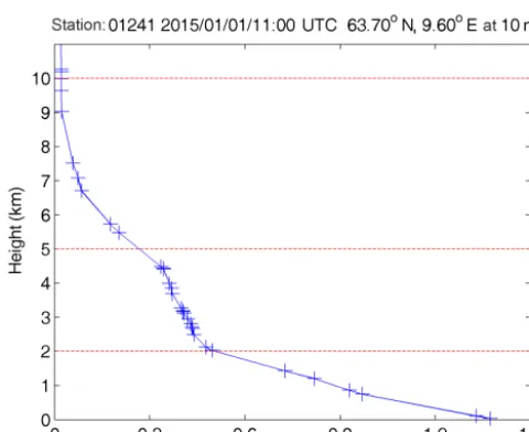
Figure 11. Uncertainty of ZWD with respect to height at sta-tion 01241 (63.70◦N, 9.60◦E at 10 m) at 11:00 UTC on 1 Jan-uary 2015.

tainty of ZWD derived from radiosonde data. Rózsa (2014) showed that the uncertainty of ZWD is±1.5 mm in the case of the Vaisala RS-92 radiosondes in central and eastern Eu-rope. However, this uncertainty is only valid for the ZWD calculated from the height of the lowest layer and is lim-ited to Europe. Using the same uncertainties of radiosonde

meteorological data given by the technical specification of the radiosonde and the algorithm proposed by Rozsa (2014), we calculated the ZWD uncertainty for all heights in all ra-diosonde stations. Figure 11 shows the uncertainty of ZWD with respect to the height for radiosonde station 01241 lo-cated in Orland, Norway (63.70◦N, 9.60◦E at 10 m). We can see that the uncertainty of ZWD is less than±1.5 mm near the height of 0 m and decrease quickly with increasing height. The global mean uncertainties of ZWD in all stations in the three height intervals are±1.3,±0.7, and±0.2 mm, respectively, indicating the high accuracy of ZWD derived from radiosonde data.

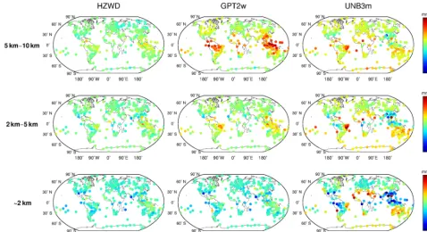
Figure 12.Global distributions of bias for the three models (HZWD, GPT2w, and UNB3m) compared to 2015 radiosonde data.

Figure 13.Global distributions of RMSE for the three models (HZWD, GPT2w, and UNB3m) compared to 2015 radiosonde data.

noting that the bias and RMSE of the HZWD model and the GPT2w model are both larger than those of the results from ECMWF data in Table 2. The reason is that the HZWD

Figure 14.RMSEs in ZWD estimates of the three models (HZWD, GPT2w, and UNB3m) for radiosonde station 01241 over the year 2015.

bias of the UNB3m model decreases, and the RMSE between 2 and 5 km and between 5 and 10 km are less than those in Table 2. It may be due to the fact that most of the radiosonde stations are in the Northern Hemisphere, accounting for more than 60 % (192/318) of the total, which has a positive im-pact on the test results for the UNB3m model based on North American meteorological data.

Figure 12 shows the global distributions of bias for the three models within the three height intervals, and Fig. 13 shows the global distributions of RMSE for the three models. As can be seen from Fig. 12, the three models show a poorer performance in low-latitude areas than in mid- and high-latitude areas for all height intervals, similar to the results in Sect. 4.1. Within the 5 to 10 km interval, the bias of the GPT2w model is large and positive in the equatorial region, indicating that the ZWD of the GPT2w at this height is sig-nificantly overestimated, and the global bias of the UNB3m model in this height interval is positive, also indicating an overestimate of the ZWD in the UNB3m model. The bias of the HZWD model does not show obvious regional dif-ferences with respect to height, and the overall distribution of HZWD model bias has no tendency to either the positive or negative. Figure 13 further illustrates the precision of the HZWD model. The global RMSE distributions of the HZWD model are similar to that of GPT2w model below 2 km and between 2 and 5 km, but the precision of the HZWD model is slightly better. Combining this with the bias distribution of the GPT2w model in Fig. 12, the GPT2w model also has a large RMSE near the Equator in the 5 to 10 km interval, which shows that the GPT2w model is unstable at high height

in low-latitude areas. The precision of the UNB3m model is poorer than that of both the HZWD and GPT2w models. Be-low 2 km, the UNB3m model reaches decimetre-level preci-sion near the Equator, and even exceeds 12 cm in some areas: the distribution of north–south heterogeneity remains obvi-ous.

These results validate the spatial stability of the precision of the HZWD model; furthermore the temporal stability of the model precision is verified next. Figure 14 shows the results of ZWD corrections of the three models for the ra-diosonde station 01241 for the whole of 2015. It can be seen from Fig. 14 that the HZWD model and the GPT2w model are relatively stable throughout the year, while the correc-tion performance of the UNB3m model in 2015 is worse than those of the HZWD and GPT2w models. The proba-ble reason for this is that the UNB3m model only takes into account the annual variations in the metrological elements with a fixed phase, resulting in precision instability through-out the year. The improved performance arising from use of the HZWD model, compared to that arising from use of the GPT2w model, is more apparent with increasing height: this shows that modelling ZWD piecewise with height can ef-fectively approximate the real ZWD profile and improve the precision of ZWD estimation.

5 Conclusions

characteristics of vertical variation of wet delay are analysed. The troposphere is divided into three height intervals: below 2 km, 2 to 5 km, and 5 to 10 km according to different trends (10 km is assumed to represent the empirical tropopause). A quadratic polynomial and two exponential functions are used to describe the variation of wet delay within each of the three intervals. Based on the monthly mean data of ECMWF ZWD from 2001 to 2010, a global ZWD model with spa-tial resolution of 5◦×5◦was established with height fitting followed by periodic fitting. Using the ECMWF ZWD data for 2015, the annual average RMSEs in the HZWD model are 23.8, 13.1, and 2.6 mm in the below 2 km, 2 to 5 km, and 5 to 10 km height intervals, respectively, which is far supe-rior to the performance of the UNB3m model. Compared to the currently most accurate wet delay empirical model (the GPT2w model), the precisions within the three height in-tervals improved by 6 % (1.4 mm), 6 % (0.9 mm), and 32 % (1.2 mm), respectively. The improvements will result in pre-cision improvements of 2.8, 1.8, and 2.4 mm respectively in height estimates in real-time aircraft positioning. The testing results of radiosonde data from 318 stations in 2015 show that the annual average RMSEs of the HZWD model are 30.1, 15.8, and 3.5 mm, which are 2 % (0.6 mm), 5 % (0.9 mm), and 33 % (1.7 mm) better than those of the GPT2w model, respectively, corresponding to height error reduction of 1.2, 1.8, and 3.4 mm in real-time aircraft positioning. Con-sidering the ZWD fields (0.126, 0.0489, and 0.0111 m) in the three height intervals, the precision improvements at the top layer are especially significant, which accounts for about 15 % of the corresponding ZWD field. Moreover, compared with the GPT2w and UNB3m models, the HZWD model of-fers the highest spatio-temporal stability. With higher pre-cision of ZWD estimates and fewer model parameters, the HZWD model is more efficient than the GPT2w model.

The HZWD model offers good precision stability in the vertical direction and can meet the requirements of ZWD correction at different heights within the troposphere; how-ever, it can be seen that neither the HZWD nor the GPT2w models, i.e. those non-meteorological parameter-based mod-els, performed well in the lowest region of the troposphere. In addition, compared with GPT2w, HZWD model is a closed model with a limitation to facilitate on-site meteorological observations. Further research is required to assess the varia-tion and factors influencing the wet delay and to explore the possibility of incorporation of on-site meteorological data.

Data availability. The ERA-Interim data can be downloaded from ECMWF (Dee et al., 2011). The radiosonde data can be downloaded from the IGRA (ftp://ftp.ncdc.noaa.gov/pub/data/igra/, last access: 1 November 2018) (NOAA, 2018).

Author contributions. YY and YH contributed to the conception of the study. YY contributed significantly to the data analysis and

manuscript preparation. YH performed the model validation and wrote the manuscript.

Competing interests. The authors declare that they have no conflict of interest.

Acknowledgements. The authors would like to thank the ECMWF and IGRA for providing relevant data. We thank the reviewers for their insightful comments and constructive suggestions. This research was supported by the National Key Research and Development Program of China (2016YFB0501803) and the National Natural Science Foundation of China (41574028) and Key Laboratory of Geospace Environment and Geodesy, Ministry of Education, Wuhan University (16-02-03).

Edited by: Marc Salzmann

Reviewed by: Jakub Kalita and M. Joana Fernandes

References

Askne, J. and Nordius, H.: Estimation of tropospheric delay for mi-crowaves from surface weather data, Radio Sci., 22, 379–386, 1987).

Bevis, M., Businger, S., Herring, T. A., Rocken, C., Anthes, R. A., and Ware, R. H.: GPS meteorology: Remote sensing of atmo-spheric water vapor using the Global Positioning System, J. Geo-phys. Res.-Atmos., 97, 15787–15801, 1992.

Bevis, M., Businger, S., Chiswell, S., Herring, T. A., Anthes, R. A., Rocken, C., and Ware, R. H.: GPS meteorology: Mapping zenith wet delays onto precipitable water, J. Appl. Meteorol., 33, 379– 386, 1994.

Böhm, J. and Schuh, H. (Eds.): Atmospheric effects in space geodesy, Berlin, Springer, Vol. 5, 6–7, 2013.

Böhm, J., Möller, G., Schindelegger, M., Pain, G., and Weber, R.: Development of an improved empirical model for slant delays in the troposphere (GPT2w), GPS Solut., 19, 433–441, 2015. Collins, P., Langley, R., and LaMance, J.: Limiting factors in

tro-pospheric propagation delay error modelling for GPS airborne navigation, Proc. Inst. Navig. 52nd Ann. Meet, 3, http://gauss2. gge.unb.ca/papers.pdf/ion52am.collins.pdf, 1996.

Davis, J. L., Herring, T. A., Shapiro, I. I., Rogers, A. E. E., and Elgered, G.: Geodesy by radio interferometry: Effects of atmo-spheric modeling errors on estimates of baseline length, Radio Sci., 20, 1593–1607, 1985.

Dee, D. P., Uppala, S. M., Simmons, A. J., et al.: The ERA-Interim reanalysis: Configuration and performance of the data assimila-tion system, Q. J. Roy. Meteor. Soc., 137, 553–597, 2011. Fernandes, M. J., Nunes, A. L., and Lázaro, C.: Analysis and

inter-calibration of wet path delay datasets to compute the wet tropo-spheric correction for CryoSat-2 over ocean, Remote Sens., 5, 4977–5005, 2013.

Fernandes, M. J., Lázaro, C., Nunes, A. L., and Scharroo, R.: Atmo-spheric corrections for altimetry studies over inland water, Re-mote Sens., 6, 4952–4997, 2014.

ap-plications using numerical weather models, J. Geophys. Res.-Atmos., 113, https://doi.org/10.1029/2008jd010503, 2008. Hopfield, H. S.: Tropospheric effect on electromagnetically

mea-sured range: Prediction from surface weather data, Radio Sci., 6, 357–367, 1971.

Jin, S., Park, J. U., Cho, J. H., and Park, P. H.: Seasonal variability of GPS-derived zenith tropospheric delay (1994– 2006) and climate implications, J. Geophys. Res.-Atmos., 112, https://doi.org/10.1029/2006jd007772, 2007.

Kouba, J.: Implementation and testing of the gridded Vienna Map-ping Function 1 (VMF1), J. Geodesy, 82, 193–205, 2008. Krueger, E., Schueler, T., Hein, G. W., Martellucci, A., and

Blarzino, G.: Galileo tropospheric correction approaches devel-oped within GSTB-V1, in: Proc. ENC-GNSS, Vol. 1619, 2004. Krueger, E., Schueler, T., and Arbesser-Rastburg, B.:. The standard

tropospheric correction model for the European satellite naviga-tion system Galileo, Proc. General Assembly URSI, 2005. Lagler, K., Schindelegger, M., Böhm, J., Krásná, H., and Nilsson,

T.: GPT2: Empirical slant delay model for radio space geodetic techniques, Geophys. Res. Lett., 40, 1069–1073, 2013.

Leandro, R., Santos, M. C., and Langley, R. B.: UNB neutral atmo-sphere models: development and performance, Proc. ION NTM, 52, 564–573, 2006.

Möller, G., Weber, R., and Böhm, J.: Improved troposphere blind models based on numerical weather data, Navigation, 61, 203– 211, 2014.

Nafisi, V., Madzak, M., Böhm, J., Ardalan, A. A., and Schuh, H.: Ray-traced tropospheric delays in VLBI analysis, Radio Sci., 47, 1–17, 2012.

Niell, A. E.: Global mapping functions for the atmosphere delay at radio wavelengths, J. Geophys. Res.-Sol. Ea., 101, 3227–3246, 1996.

Nilsson, T. and Elgered, G.: Long-term trends in the at-mospheric water vapor content estimated from ground-based GPS data, J. Geophys. Res.-Atmos., 113, https://doi.org/10.1029/2008jd010110, 2008.

NOAA: Radiosonde data, available at: ftp://ftp.ncdc.noaa.gov/, last access: 1 November 2018.

Rózsa, S. Z.: Uncertainty considerations for the comparison of wa-ter vapour derived from radiosondes and GNSS[M]//Earth on the Edge: Science for a Sustainable Planet, Springer Berlin Heidel-berg, 65–78, 2014.

RTCA: Minimum Operational Performance Standards For Global Positioning System/Satellite-Based Augmentation System Air-borne Equipment, Radio Technical Commission for Aeronautics, SC-159, publication DO-229E, Washington, DC, 2016. Saastamoinen, J.: Introduction to practical computation of

astro-nomical refraction, Bull. Géodésique, 106, 383–397, 1972. Schüler, T.: The TropGrid2 standard tropospheric correction model,

GPS Solut., 18, 123–131, 2014.

Song, S., Zhu, W., Chen, Q., and Liou, Y.: Establishment of a new tropospheric delay correction model over China area, Sci. China Phys. Chem., 54, 2271–2283, 2011.

Stum, J., Sicard, P., Carrere, L., and Lambin, J.: Using objective analysis of scanning radiometer measurements to compute the water vapor path delay for altimetry, IEEE T. Geosci. Remote, 49, 3211–3224, 2011.

Vieira, T., Fernandes, M. J., and Lázaro, C.: Analysis and retrieval of tropospheric corrections for cryosat-2 over inland waters, Adv. Space Res., 62, 1479–1496, 2018.