A numerical procedure based on 1D-IRBFN and local MLS-1D-IRBFN methods for fluid-structure interaction analysis

A numerical procedure based on 1D-IRBFN and local

MLS-1D-IRBFN methods for fluid-structure interaction

analysis

D. Ngo-Cong1,2, N. Mai-Duy1, W. Karunasena2and T. Tran-Cong1,3

Abstract: The partition of unity method is employed to incorporate the mov-ing least square (MLS) and one dimensional-integrated radial basis function (1D-IRBFN) techniques in a new approach, namely local MLS-1D-IRBFN or LMLS-1D-IRBFN. This approach leads to sparse system matrices and offers a high level of accuracy as in the case of 1D-IRBFN method. A new numerical procedure based on the 1D-IRBFN method and LMLS-1D-IRBFN approach is presented for a so-lution of fluid-structure interaction (FSI) problems. A combination of Chorin’s method and pseudo-time subiterative technique is presented for a transient solution of 2-D incompressible viscous Navier-Stokes equations in terms of primitive vari-ables. Fluid domains are discretised by using Cartesian grids. The fluid solver is first verified through a solution of mixed convection in a lid-driven cavity with a hot lid and a cold bottom wall. The structural solver is verified with an analytical solution of forced vibration of a beam. The Newmark’s method is employed for the forced vibration analysis of the beam based on the Euler-Bernoulli theory. The FSI numerical procedure is then applied to simulate flows in a lid-driven open-cavity with a flexible bottom wall.

Keywords: Fluid-structure interaction; moving boundary; transient analysis; pseudo-time subiterative technique; integrated radial basis function; Cartesian grid.

1 Introduction

Fluid-structure interaction (FSI) plays a central role in several engineering prob-lems such as aircraft wing flutter [Dubcova, Feistauer, Horacek, and Svacek (2008)],

1_{Computational Engineering and Science Research Centre, Faculty of Engineering and Surveying,} The University of Southern Queensland, Toowoomba, QLD 4350, Australia.

2_{Centre of Excellence in Engineered Fibre Composites, Faculty of Engineering and Surveying, The} University of Southern Queensland, Toowoomba, QLD 4350, Australia.

bridge flutter [Ge and Xiang (2008)], blood flows [Fernández, Gerbeau, and Grand-mont (2007)], design of helicopter rotors [Xiong and Yu (2007)]. Therefore, FSI is a very attractive topic and FSI analysis is the key for solving those kinds of prob-lems. FSI is also a challenge for numerical modelling. To solve FSI problems, one needs to consider the governing equations for fluid and structure, and geometrical compatibility and equilibrium conditions at the interfaces between fluid and struc-tural domains. Some FSI behaviours can converge to a steady-state solution, others can be oscillatory or even unstable.

There are two main approaches for solving FSI problems, namely monolithic meth-ods [Rugonyi and Bathe (2001); Heil (2004); Liew, Wang, Zhang, and He (2007)] and partitioned methods [Farhat and Lesoinne (1998); Piperno (1997)]. Partitioned procedures are usually appropriate for weak interaction between the fluid and the structure while the monolithic procedure is chosen to be effective for solving FSI problems with a strong interaction. In the monolithic approach, the fluid and struc-tural equations are solved simultaneously. This approach may lead to two draw-backs (i) an increase in the number of degrees of freedom (DOFs) and (ii) an ill-conditioned system matrix. Liew, Wang, Zhang, and He (2007) developed a monolithic approach based on the fluid pressure Poisson equation to solve the hy-droelasticity problem of an incompressible viscous fluid with a elastic body that is vibrating due to flow excitation. The flow was modelled with low-order velocity-pressure finite elements while the structure was represented by means of a Galerkin finite element formulation.

In the partitioned approach, the fluid and structural fields are solved separately and the solution variables are transferred at the interfaces of the fluid and structural do-mains. The major advantage of this approach is the flexibility to choose different solvers for each field. However, the approach introduces a time delay which results in non-physical energy dissipation [Farhat and Lesoinne (1998)]. Piperno (1997) introduced coupling staggered procedures with a structural predictor for a tran-sient solution of a supersonic panel flutter using dynamic mesh and finite volume methods (FVM) based on the arbitrary-Lagrangian-Eulerian (ALE) formulation. Their procedures do not satisfy continuity of the structural and fluid grid displace-ments/velocities at the moving interface, but allow an exact numerical exchange of momentum through the interface.

staggered FSI simulations where incompressible flows are considered. Bathe and Zhang (2009) presented a numerical procedure to adapt and repair the fluid mesh for solving this FSI problem using the ALE formulation. The fully adaptive solu-tion of transient flow are too expensive and may lead to large computasolu-tional errors during the time integration. Therefore, they first solved a steady flow in a lid-driven cavity at the maximum velocity of the lid to obtain an adaptive mesh. This mesh is then employed for the transient solution of the FSI system. Al-Amiri and Khanafer (2011) investigated a steady laminar mixed convection heat transfer in a lid-driven cavity with a flexible bottom wall using a finite element formulation based on the Gelerkin method of weighted residuals.

par-tition of unity framework to incorporate the moving least square and 1D-IRBFN techniques in an approach that produces a very sparse system matrix and offers as a high level of accuracy as that of the 1D-IRBFN.

The present work is concerned with the development of a new numerical proce-dure based on the 1D-IRBFN and local MLS-1D-IRBFN methods for solving FSI and moving boundary problems such as flows in a lid-driven open-cavity with a flexible bottom wall. The fluid flow is governed by 2-D incompressible viscous Navier-Stokes equations in terms of primitive variables and the motion of the bot-tom wall is described by using the Euler-Bernoulli theory. The present fluid solver is first verified through a benchmark solution of mixed convection in a lid-driven cavity with a hot moving lid and a cold stationary bottom wall. Torrance, Davis, Eike, Gill, Gutman, Hsui, Lyons, and Zien (1972) first numerically studied this kind of problem and found that the interaction of the shear driven flow due to the lid motion and natural convection due to the buoyancy effect makes the flow be-haviour complicated and different from those driven by the two effects separately. Iwatsu, Hyun, and Kuwahara (1993) studied mixed convection in a lid-driven cavity with a hot moving top wall and a cold stationary bottom wall using finite different method (FDM). Sharif (2007) investigated the mixed convection heat transfer in in-clined cavities using the FVM with a second-order upwind differencing scheme to discretise convection terms and central differencing scheme to discretise diffusion terms. Recently, Cheng (2011) employed a fourth-order accurate compact form and pseudo time iteration methods for simulations of mixed convection in a 2-D lid-driven cavity using the stream function, vorticity and temperature formulation.

The present paper is organised as follows. Section 2 briefly reproduces the 1D-IRBFN and local MLS-1D-1D-IRBFN techniques. The governing equations for struc-ture, 2-D incompressible viscous flows and FSI are presented in Section 3. Sec-tion 4 describes the discretisaSec-tion of the governing equaSec-tions, the details of deter-mination of variable values at “freshly cleared" nodes (defined later in section 4.3) and a sequentially staggered algorithm for FSI analysis. Several numerical exam-ples are investigated using the present numerical procedure in Section 5. Section 6 concludes the paper.

2 1D-IRBFN and local MLS-1D-IRBFN methods

2.1 1D-IRBFN methods

The 1D-IRBFN methods [Mai-Duy and Tanner (2007)] including 1D-IRBFN-2 and 1D-IRBFN-4 schemes are briefly described here.

2.1.1 Second-order 1D-IRBFN (1D-IRBFN-2 scheme)

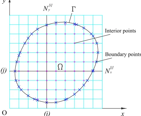
Consider an x-grid line, e.g.[j], as shown in Fig. 1. The variation of u along this line is sought in the IRBF form. The second-order derivative of u is decomposed into RBFs; the RBF network is then integrated once and twice to obtain the expressions for the first-order derivative of u and the solution u itself,

∂2_u(x)

∂x2 =

Nx[j]

∑

w(i)G(i)(x) =

Nx[j]

∑

w(i)H_[(₂i)_](x), (1)

∂u(x)

∂x =

Nx[j]

∑

w(i)H_[(₁i_])(x) +c1, (2)

u(x) =

Nx[j]

∑

w(i)H_[(₀i_])(x) +c1x+c2, (3)

where Nx[j] is the number of nodes on the grid line [j]; {w(i)}N [j]

x

i=1 RBF weights to

be determined;G(i)(x) N

[j]

x

i=1=

n

H_[(₂i)_](x)oN

[j]

x

i=1known RBFs; H

(i) [1](x) =

R

H_[(₂i)_](x)dx;

H_[(₀i)_](x) =R

H_[(₁i)_](x)dx; and c1and c2integration constants which are also unknown.

An example of RBF, used in this work, is the multiquadrics G(i)(x) =p(x−x(i)₎2_+a(i)2_, a(i)is the RBF width determined as a(k)=βd(k),β a positive factor, and d(k)the distance from the kthcenter to its nearest neighbour.

2.1.2 Fourth-order 1D-IRBFN (1D-IRBFN-4 scheme)

function itself,

∂4_u(x)

∂x4 =

Nx[j]

∑

w(i)G(i)(x) =

Nx[j]

∑

w(i)H_[(₄i)_](x), (4)

∂3_u(x)

∂x3 =

Nx[j]

∑

w(i)H_[(₃i)_](x) +c1, (5)

∂2_u(x)

∂x2 =

Nx[j]

∑

w(i)H_[(₂i_])(x) +c1x+c2, (6)

∂u(x)

∂x =

Nx[j]

∑

w(i)H_[(₁i_])(x) +c1 2x

2_+c

2x+c3, (7)

u(x) =

Nx[j]

∑

w(i)H_[(₀i)_](x) +c1 6x

3₊c2 2x

2_+c

3x+c4, (8)

whereG(i)(x) N

[j]

x

i=1=

n

H_[(₄i_])(x)oN

[j]

x

i=1are known RBFs; H

(i) [3](x) =

R

H_[(₄i)_](x)dx; H_[(₂i_])(x) =

R

H_[(₃i_])(x)dx; H_[(₁i)_](x) =R

H_[(₂i)_](x)dx; H_[(₀i)_](x) =R

H_[(₁i_])(x)dx; and c1,c2,c3and c4 in-tegration constants which are also unknown.

2.2 Local moving least square - one dimensional integrated radial basis func-tion network technique

A schematic outline of the LMLS-1D-IRBFN method is depicted in Fig. 2. The proposed method with 3-node support domains (n=3) and 5-node local 1D-IRBF networks (ns=5) is presented here. On an x-grid line[l], a global interpolant for

the field variable at a grid point xiis sought in the form

u(xi) = n

∑

φj(xi)u[j](xi), (9)

whereφ¯j n

j=1is a set of the partition of unity functions constructed using MLS approximants [Liu (2003)]; u[j](xi)the nodal function value obtained from a local

interpolant represented by a 1D-IRBF network [j]; n the number of nodes in the support domain of xi. In (9), MLS approximants are presently based on linear

polynomials, which are defined in terms of 1 and x. It is noted that the MLS shape functions possess a so-called partition of unity properties as follows.

n

∑

Relevant derivatives of u at xican be obtained by differentiating (9)

∂u(xi)

∂x =

n

∑

∂_φ¯_j(xi)

∂x u

[j]_(x

i) +φ¯j(xi)∂

u[j](xi)

∂x

!

, (11)

∂2_u(x

i)

∂x2 =

n

∑

∂2φ_¯

j(xi)

∂x2 u

[j]_(x

i) +2

∂_φ¯_j(xi) ∂x

∂u[j](xi)

∂x +φ¯j(xi)

∂2_u[j]_(x

i)

∂x2

!

, (12)

where the values u[j](xi),∂u[j](xi)/∂x and∂2u[j](xi)/∂x2 are calculated from

1D-IRBFN networks with nsnodes.

Full details of the LMLS-1D-IRBFN method can be found in [Ngo-Cong, Mai-Duy, Karunasena, and Tran-Cong (2012)].

3 Governing equations for fluid, structure and fluid-structure interaction

In this study, the FSI problem of flow in a lid-driven open-cavity with a flexible bot-tom wall [Förster, Wall, and Ramm (2007); Bathe and Zhang (2009)] is considered. The bottom wall is modelled as a flexible beam using the Euler-Bernoulli beam the-ory. The fluid is described by the 2-D Navier-Stokes equations of incompressible viscous flow in terms of primitive variables.

3.1 Governing equations for forced vibration of a beam

The equation of motion for forced lateral vibration of a beam is based on the Euler-Bernoulli beam theory. This is a small-deflection theory and therefore some error will be incurred due to the neglect of the geometric non-linear term when the de-flection is actually not small [Spoon and Grant (2011)]. Our purpose here is to demonstrate our FSI analysis procedure and we will ignore the non-linear term here for the following reason. As shown later in the numerical results section, the actual maximum central deflection of the beam is about 14.71% of the beam length in the worst case of simply-supported boundary conditions and therefore the error is less than 10% [Spoon and Grant (2011)]. In the case of clamped boundary con-ditions, the error is less than 1.3% since the maximum deflection is about 4.37% of the beam length. The equation of motion is given by [Rao (2004)]

EI∂ 4_w

∂x4 +ρsA

∂2_w

∂t2 = f(x,t). (13)

where w is the lateral deflection of the beam; t the time; E Young’s modulus; I the moment of inertia; A the cross-section area; ρsmaterial density of the beam; and

• Simply supported case:

w=0,∂

2_w

∂x2 =0. (14)

• Clamped case:

w=0,∂w

∂x =0. (15)

3.2 Governing equations for 2-D incompressible viscous flows

The dimensional conservative form of the 2-D Navier-Stokes equations of incom-pressible viscous flow in terms of primitive variables is written in xy-Cartesian system as [Bathe and Zhang (2009)]

∂u ∂x+

∂v

∂y =0, (16)

ρf∂

u ∂t +ρf

∂u2 ∂x +ρf

∂uv

∂y =−

∂p ∂x+µ

∂2_u

∂x2+

∂2_u

∂y2

, (17)

ρf∂

v ∂t +ρf

∂uv ∂x +ρf

∂v2

∂y =−

∂p ∂y+µ

∂₂

v ∂x2+

∂2_v

∂y2

, (18)

where u, v and p are velocity components and static pressure of the fluid, respec-tively;ρf the fluid density; andµ the dynamic viscosity of the fluid.

3.3 Coupled equations for fluid-structure interaction

The geometrical compatibility conditions at the interface Γbetween the fluid and structural domains are given by

rΓ(t) =wΓ(t), (19)

˙rΓ(t) =w˙Γ(t), (20)

where rΓand wΓare the displacement vectors of the fluid and structure at the inter-faceΓ, respectively; and ˙rΓand ˙wΓthe velocity vectors of the fluid and structure at the interfaceΓ, respectively.

The equilibrium conditions can be described as follows.

hΓ_f(t) +hΓ_s(t) =0, (21)

4 Numerical procedures

In this section, the fractional-step projection method proposed by Chorin (1967) is described for solving the system of equations (16)-(18) with the use of 1D-IRBFN and LMLS-1D-IRBFN methods for spatial discretisation. The combination of the fractional-step projection method and the subiterative technique [Jameson (1991); Melson, Sanetrik, and Atkins (1993)] is presented to solve transient flow problems. The details of determination of variable values at “freshly cleared" nodes and a sequentially staggered algorithm for FSI analysis are also given here.

4.1 Fractional-step projection method (Chorin’s method)

• First step: Determine intermediate velocities u∗and v∗by ignoring the pres-sure term and incompressibility. Convection and diffusion terms are discre-tised explicitly at time level(n)using the 1D-IRBFN method.

ρf

u∗−u(n)

∆t =−ρf

∂(u(n)₎2

∂x −ρf

∂u(n)v(n)

∂y +µ

"

∂2_u(n)

∂x2 +

∂2_u(n) ∂y2

#

, (22)

ρf

v∗−v(n)

∆t =−ρf

∂u(n)v(n)

∂x −ρf

∂(v(n)₎2

∂y +µ

"

∂2_v(n) ∂x2 +

∂2_v(n) ∂y2

#

. (23)

• Second step: Solve a Poisson equation for the pressure at time level(n+1)

∂2_p(n+1)

∂x2 +

∂2_p(n+1)

∂y2 =

ρf

∆t

∂

u∗

∂x +

∂v∗ ∂y

. (24)

It is noted that the LHS of (24) is discretised using the local MLS-1D-IRBFN method while the RHS is calculated with the 1D-IRBFN method. The pro-cess results in a sparse system of equations, which is then economically solved by the LU decomposition technique.

Neumann boundary conditions for pressure are given by

∂p(n+1)

∂x =ρf

u∗−u(n)

∆t , (25)

∂p(n+1)

∂y =ρf

v∗−v(n)

Then, the velocities u(n+1)and v(n+1)are determined as

u(n+1)=u∗−∆t

ρf

∂p(n+1)

∂x , (27)

v(n+1)=v∗−∆t

ρf

∂p(n+1)

∂y . (28)

For irregular domain problems, when determining the derivatives of pressure w.r.t. y on the curved boundary through Equation (26), the values of v∗ on the curved boundary are unknown and can be determined by using a 1D-IRBFN extrapolant from the v∗values at the interior points as follows.

v∗(yB) =HˆBHˆ−1I vˆ

∗

I, (29)

where yB is the y-coordinate of node B on the curved boundary as shown in Fig. 3;

ˆ

v∗_I =(v∗)(1)_,(v∗₎(2)_{, ...,(v}∗₎(Ny[m]−1)

T

;

ˆ

HB=h H_[(₀1_])(yB) H_[(₀2_])(yB) ... H

(Ny[m]−1)

[0] (yB) yB 1

i

;

ˆ HI=

       

H_[(₀1_])(y1) H_[(₀2_])(y1) ... H

(Ny[m]−1)

[0] (y1) y1 1

H_[(₀1_])(y2) H_[(₀2_])(y2) ... H

(Ny[m]−1)

[0] (y2) y2 1

... ... ... ... ... ...

H_[(₀1_])(y_N[m]

y −1) H

(2)

[0](yNy[m]−1) ... H (Ny[m]−1)

[0] (yNy[m]−1) yNy[m]−1 1

        ;

in which Ny[m] is the number of grid nodes on the y-grid line [m] excluding the

node on the curved boundary. The values of u∗ on the curved boundary can be determined in a similar fashion.

Dirichlet boundary condition for pressure

Making use of Equation (3) for pressure values at interior points of an x-grid line [j]and Equation (2) for first-order derivatives of pressure at the ends of that grid line results in



 

ˆ pI

∂p(1)

∂x

∂p(N[xj])

∂x   = _ˆ HI ˆ K ˆ w ˆ c , (30) or ˆ w ˆ c = _ˆ HI ˆ K −1    ˆ pI

∂p(1)

∂x

∂p(Nx[j])

∂x 



where

ˆ pI=

p(2),p(3), ...,p(Nx[j]−1)

T ; ˆ HI=       

H_[(₀1_])(x2) H_[(₀2_])(x2) ... H(N

[j]

x )

[0] (x2) x2 1

H_[(₀1_])(x3) H_[(₀2_])(x3) ... H(N

[j]

x )

[0] (x3) x3 1

... ... ... ... ... ...

H_[(₀1_])(x

Nx[j]−1) H (2)

[0] (xNx[j]−1) ... H (Nx[j])

[0] (xNx[j]−1) xNx[j]−1 1

       ; ˆ K=  

H_[(₁1_])(x1) H_[(₁2_])(x1) ... H(N

[j]

x )

[1] (x1) 1 0

H_[(₁1_])(x

Nx[j]) H (2)

[1](xNx[j]) ... H (Nx[j])

[1] (xNx[j]) 1 0



;

and ∂p(1)/∂x and∂p(Nx[j])_/∂_{x are calculated through Equation (25). From}

Equa-tion (3), pressure values at the ends of the x-grid line[j]can be defined by

p(1)

p(Nx[j])

!

=HBˆ ˆ w ˆ c , (32) where ˆ HB=





H_[(₀1_])(x1) H_[(₀2_])(x1) ... H(N

[j]

x )

[0] (x1) x1 1

H_[(₀1_])(x

Nx[j]) H (2)

[0](xNx[j]) ... H (Nx[j])

[0] (xNx[j]) xNx[j] 1



.

By substituting Equation (31) into Equation (32), the boundary pressure values at both ends of the grid line[j]are expressed in terms of the values of pressure at interior points and derivatives of pressure at both ends of the grid line[j]as follows.

p(1)

p(Nx[j])

!

=_HBˆ _ˆ HI ˆ K −1    ˆ pI

∂p(1)

∂x

∂p(Nx[j])

∂x 



. (33)

The boundary pressure values at both ends of y-grid lines can be determined in a similar manner.

4.2 Combination of fractional-step projection method and subiterative tech-nique

time-step limitations which leads to a high computational cost when solving mov-ing boundary problems. Jameson (1991) and Melson, Sanetrik, and Atkins (1993) presented subiterative techniques within the context of a multigrid methodology to allow a large physical time step with the use of an explicit code. Rumsey, Sanetrik, Biedron, Melson, and Parlette (1996) combined the subiterative technique with an explicit central-difference code and an implicit upwind code for solving un-steady Navier-Stokes equations. The combination of the fractional-step projection method and the subiterative technique are now presented here. The temporal terms of Equations (17) and (18) are discretised using the backward Euler scheme while the convection and diffusion terms are treated implicitly, which results in

ρfu (n+1)_−u(n)

∆t =−ρf

∂(u(n+1)₎2 ∂x −ρf∂

u(n+1)_v(n+1)

∂y −

∂p(n+1)

∂x

+µh∂2u(n+1)

∂x2 +∂ 2_u(n+1)

∂y2

i

, (34)

ρfv (n+1)_−v(n)

∆t =−ρf∂u

(n+1)_v(n+1)

∂x −ρf

∂(v(n+1)₎2

∂y −

∂p(n+1)

∂y

+µh∂2v(n+1)

∂x2 +∂ 2_v(n+1)

∂y2

i

. (35)

Pseudo-time derivative terms are added into Equations (34) and (35) as

ρ

(n+1)_−u(n)

∆t +

ρ

u

∂τ =−

ρ

∂(u(n+1))2

∂x −

ρ

u(n+1)v(n+1)

∂y −∂p_∂(n_x+1)+

µ

2_u(n+1) ∂y2

i

,

(36)

ρ

(n+1)_−v(n)

∆t +

ρ

v

∂τ =−

ρ

(n+1)_v(n+1)

∂x −

ρ

∂(v(n+1)₎2 ∂y −∂p_∂(n_y+1) +

µ

2_v(n+1) ∂y2

i

,

(37)

whereτ is the pseudo time and t the physical time. The additional terms∂u/∂τ

and ∂u/∂τ are designed in such a way that they vanish when the values of u and v approach their correct values at time level(n+1)as follows (k is a pseudo-time level).

ρfu (n+1)_−u(n)

∆t +ρfu

(n+1,k+1)_−u(n+1,k) ∆τ =−ρf

∂(u(n+1,k)₎2 ∂x −ρf∂

u(n+1,k)_v(n+1,k)

∂y

−∂p(n_∂+_x1,k+1)+µh∂2u(n+1,k)

∂x2 +∂ 2_u(n+1,k)

∂y2

i

, (38)

ρfv (n+1)_−v(n)

∆t +ρfv

(n+1,k+1)_−v(n+1,k)

∆τ =−ρf∂u

(n+1,k)_v(n+1,k)

∂x −ρf

∂(v(n+1,k)₎2

∂y

−∂p(n_∂+_y1,k+1) +µh∂2v(n+1,k)

∂x2 +∂ 2_v(n+1,k)

∂y2

i

• First step: Determine intermediate velocities u∗and v∗by the following equa-tions. The convection and diffusion terms are explicitly calculated at pseudo-time level(k)using the 1D-IRBFN method.

ρfu

∗_−u(n+1,k) ∆τ =−ρf

∂(u(n+1,k)₎2 ∂x −ρf∂

u(n+1,k)_v(n+1,k)

∂y

+µh∂2u_∂(n_x+21,k)+∂ 2_u(n+1,k)

∂y2

i ,

(40)

ρfv

∗_−v(n+1,k)

∆τ =−ρf∂u

(n+1,k)_v(n+1,k)

∂x −ρf

∂(v(n+1,k)₎2

∂y

+µh∂2v(n+1,k)

∂x2 +∂ 2_v(n+1,k)

∂y2

i

. (41)

• Second step: Solve a Poisson equation for the pressure p(n+1,k+1)

∂2_p(n+1,k+1)

∂x2 +

∂2_p(n+1,k+1)

∂y2 =

ρf

∆τ

∂

u∗

∂x +

∂v∗ ∂y

, (42)

The LHS of (42) is discretised using the local MLS-1D-IRBFN method while the RHS is calculated with the 1D-IRBFN method. Neumann boundary con-ditions for pressure are given by

∂p(n+1,k+1)

∂x =−ρf

u(n+1,k)−u(n)

∆t −ρf

u(n+1,k)−u∗

∆τ , (43)

∂p(n+1,k+1)

∂y =−ρf

v(n+1,k)−v(n)

∆t −ρf

v(n+1,k)−v∗

∆τ . (44)

Then, velocities u(n+1,k+1)and v(n+1,k+1)are determined as follows.

u(n+1,k+1)=kt −

1 ρf

∂p(n+1,k+1)

∂x +

u(n)

∆t +

u∗ ∆τ

!

, (45)

v(n+1,k+1)=kt −

1 ρf

∂p(n+1,k+1)

∂y +

v(n) ∆t +

v∗ ∆τ

!

, (46)

• Third step: Check convergence criterion for u,v and p

CMu= s

Nip ∑

i=1

u(_in+1,k+1)−u(_in+1,k)2

s Nip

∑

i=1

u(_in+1,k+1)

2

<T OL, (47)

CMv= s

Nip ∑

i=1

v(_in+1,k+1)−v(_in+1,k)2

s Nip

∑

i=1

v(_in+1,k+1)

2

<T OL, (48)

CMp= s

Nip ∑

i=1

p(_in+1,k+1)−p(_in+1,k)2

s Nip

∑

i=1

p(_in+1,k+1)

2

<T OL, (49)

where T OL is a given tolerance and presently set to be 10−7; and Nip the

number of interior points of the fluid domain. If not converged, return to the first step. Otherwise, assign u(n+1)=u(n+1,k+1), v(n+1)=v(n+1,k+1)and p(n+1)=p(n+1,k+1), then advance the physical time t.

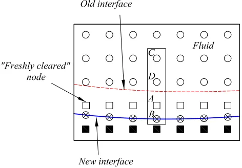
4.3 Determine variable values at “freshly cleared" nodes

“Freshly cleared" nodes are the nodes that are not inside the fluid domain at time level(n), but emerge into the fluid domain at the next time level(n+1). We need to have a “guess" value at these nodes, i.e. at pseudo-time level k=0 associated with the real time level (n+1). For this purpose, the technique presented by Udayku-mar, Mittal, Rampunggoon, and Khanna (2001) to determine values at the “freshly cleared" nodes is employed here. As shown in Fig. 4, the values at the “freshly cleared" nodes (e.g., a typical node A) are interpolated from the information at two interior nodes (nodes C and D), and one node on the boundary (node B) through the following interpolant.

uI(y) =a0+a1y+a2y2, (50)

4.4 Sequential staggered fluid-structure interaction algorithm

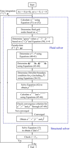
The sequentially staggered algorithm [Piperno (1997); Förster, Wall, and Ramm (2007)] is used in the present study and described as follows.

• Step 1: At the initial time(t=0s), set the displacement (w) and velocity ( ˙w)

of the bottom wall to be zero.

• Step 2: Calculate a predictor of the structural interface displacement at the new time level (w(pn+1)) using one of the following two approaches [Piperno

(1997); Förster, Wall, and Ramm (2007)].

– Approach 1: Zeroth order accurate predictor

w(pn+1)=w(n). (51)

– Approach 2: First order accurate predictor

w(pn+1)=w(n)+∆t ˙w. (52)

Then determine the grid-node system for fluid analysis based on w(pn+1).

• Step 3: Solve the fluid problem to obtain pressure distribution (pΓ) on the bottom wall with the use of ˙w as a Dirichlet boundary condition for the

ver-tical velocity (v) of fluid field.

• Step 4: Solve the structural problem for a new displacement (w) and velocity ( ˙w) of the bottom wall with consideration of the fluid load pΓ (the effect of viscous stress on the displacement of the bottom wall is much smaller than that of the pressure stress and hence neglected here). In the present study, the displacements are restricted to be small, thus there is no distinction between the material coordinates and spatial coordinates.

• Step 5: Advance physical time from level(n)to(n+1)and return to Step 2.

Steps 2-5 are repeated until a stable FSI solution is found. The flowchart of the FSI analysis procedure is described in detail as shown in Fig. 5.

5 Numerical results and discussion

for fluid flow, structural response and ultimately the response in a fluid-structure in-teraction problem. The domains of interest are discretised using uniform Cartesian grids. By using the LMLS-1D-IRBFN method to discretise the LHS of governing equations and the LU decomposition technique to solve the resultant sparse system of simultaneous equations, the computational cost is reduced.

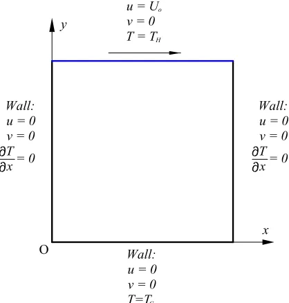
5.1 Example 1: Mixed convection in a lid-driven cavity

The fluid solver is first verified through a solution of mixed convection in a lid-driven cavity with a hot moving lid and a cold stationary bottom wall. The prob-lem geometry and boundary conditions are described in Fig. 6. With the Boussi-nesq approximation, the dimensionless form of 2-D incompressible Navier-Stokes equations in terms of primitive variables and the energy equation governing the mixed convection in the cavity are written as follows [Iwatsu, Hyun, and Kuwahara (1993)].

∂U

∂X +

∂V

∂Y =0, (53)

∂U ∂t′ +

∂U2

∂X +

∂UV

∂Y =−

∂P

∂X+

1 Re

∂2_U

∂X2+

∂2_U

∂Y2

, (54)

∂V ∂t′ +

∂UV

∂X +

∂V2

∂Y =−

∂P

∂Y +

1 Re

∂₂

V ∂X2+

∂2_V

∂Y2

+ Gr

Re2θ, (55)

∂θ ∂t′+

∂Uθ

∂X +

∂Vθ

∂Y =

1 Pr Re

∂2_θ

∂X2+

∂2_θ

∂Y2

. (56)

The variables in the equations above are nondimensionalised as

t′= t H/U0

,X= x H,Y =

y H,

U= u

U0

,V = v U0

,P= p ρfU₀2

,θ= T−TC TH−TC

,

where H is the side length of the square cavity and U0 velocity of the lid; T the temperature; and TH and TCthe hot and cold temperatures, respectively.

In these equations, the nondimensionalised parameters are the Reynolds number Re=U0H/ν, the Prandtl number Pr=ν/α (Pr is set to be 0.71 presently) and the Grashof number Gr=Ra/Pr, where Ra=gβ(TH−TC)H3/(να), ν is the

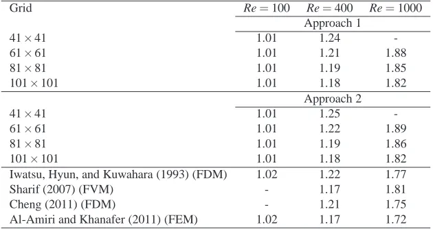
The fractional-step projection method is applied to solve this problem with a time step∆t′=10−3. Tabs. 1-3 describe the grid convergence study of the average Nus-selt number at the lid for several Grashof numbers Gr=102,104 and 106, and Reynolds numbers Re=100,400 and 1000. The LHS of pressure Poisson equa-tion (24) is discretised by using 1D-IRBFN method (Approach 1) and LMLS-1D-IRBFN method (Approach 2). The system matrix of Approach 2 is much more sparse than that of Approach 1. The obtained numerical results showed that both approaches yield the same level of accuracy. Approach 2 is used for all other com-putations in the present study in order to save the computational cost. It can be seen that the converged numerical results are in good agreement with the published re-sults of other authors. The isothermal lines and streamlines of the flow field inside the cavity at several Gr and Re numbers are depicted in Figs. 7-9.

For the case Gr=102 (Fig. 7), the forced convection effect is dominant (Ri≪1), thus the streamlines of the flow are similar to those of the classical lid-driven cavity case (readers are referred to the work of Ghia, Ghia, and Shin (1982) for Re= 100,400 and 1000. At Re=1000, the temperature gradient is steep at the region close to the bottom wall and the lid, while the temperature gradient is small at the center region of the cavity. This indicates that the fluid is well mixed for the bulk of the cavity due to the flow circulation.

For the case Gr=104 (Fig. 8), the natural convection effect is comparable to the forced convection effect at Re=100 (Ri=1), while the forced convection effect is still dominant at Re=400 and 1000 (Ri≪1). Therefore, the flow pattern is quite different at Re=100, while remains similar at Re=400 and 1000, when compared to those of the above case (Gr=102).

For the case Gr=106 (Fig. 9), the natural convection effect is stronger than the forced convection effect. The flow patterns are very different from those of the classical lid-driven cavity case for several Reynolds numbers Re=100,400 and 1000. It is observed that the heat conduction is almost uniform for the case Re= 100 and mainly occurs at the bottom and middle regions of the cavity for the cases Re=400 and 1000.

5.2 Example 2: Flow in a lid-driven open-cavity with a prescribed bottom wall motion

The problem geometry and boundary conditions are described in Fig. 10. The fluid properties and problem geometry used here are: fluid kinematic viscosityν= 0.01m2/s, fluid densityρf =1.0kg/m3, the side length of the square cavity H=1m

• Case 1: U0=1 m/s.

• Case 2: U0=1−cos(ωft)m/s.

The combination of the fractional-step projection method and subiterative tech-nique is applied to compute the transient solutions of the flow in the cavity. The grid convergence study is first conducted for the case of stationary bottom wall (w=0) and maximum velocity-loading of the lid (U0=2m/s or Re=200). Fig. 11 depicts grid-convergence behaviour of vertical and horizontal velocities along the horizontal and vertical center lines, and static pressure distribution along the sta-tionary bottom wall for the case Re=200. Grid convergence is observed and the numerical results obtained are indistinguishable for grids denser than or equal to 61×61. The contours of stream function, velocity magnitude and static pressure of the flow in the cavity for the case Re=200 are shown in Fig. 12.

Cartesian grids with a grid spacing of 1/60 are employed for the case of prescribed bottom wall motion. As shown in Fig. 13, the fluid domains are represented by Regions A and B for a convex bottom wall, by Regions A, B1and B2for a concave bottom wall. The LHS of pressure Poisson equation (42) is discretised through the following strategy. The LMLS-1D-IRBFN method is employed to discretise the term∂2p/∂x2 in Region A, while the 1D-IRBFN is used to discretise that term in Region B (or Regions B1and B2). The discretisation of the term∂2p/∂y2is carried out using the LMLS-1D-IRBFN method.

Fig. 14 presents the response of static pressure at the mid-point of the bottom wall (pM) with respect to time for Case 1. The physical time step (∆t) and pseudo time

step (∆τ) are taken to be 0.1s and 10−3s, respectively. It is noted that this response varies periodically with the same frequency as that of the bottom wall motion (= ωf/2π). Fig. 15 shows the contours of stream function, velocity magnitude and

static pressure of the flow inside the cavity for several times t=51.5,52.0,52.5 and 53.0s (within one time period) for Case 1. The corresponding numerical results for Case 2 are shown in Figs. 16 and 17.

5.3 Example 3: Forced vibration of a simply supported beam

This example deals with the dynamic behaviour of a simply supported beam subject to a harmonic external force F(t) = f0sinωt applied at x=a, as shown in Fig. 18 (where f0=0.1N,ω=2π/5 rad/s, aL=1m and a=0.5m). The problem geometry

for the simply supported beam can be described as

w=0,∂

2_w

∂x2 =0, at x=0,x=aL (57)

w=0,∂w

∂t =v0, at t=0 (58)

where v0is the initial velocity of the beam. An analytical solution to this problem can be found in [Rao (2004)].

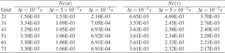
The fully discrete scheme with Newmark’s method for temporal discretisation is employed here. The spatial term is discretised by using the 1D-IRBFN-4 scheme based on a uniform grid. Tab. 4 describes the grid convergence study of deflection u and velocity v of the beam at time t=14s. For a given time step, the accuracy is not improved further when refining the grid to a certain grid size. However, the ac-curacy is greatly improved by reducing the time step. This indicates that the major numerical error is not due to the 1D-IRBFN approximation, but due to the temporal discretisation. The steady-state responses of the forced vibration system obtained by the 1D-IRBFN method are in good agreement with the analytical solution as shown in Fig. 19, using a uniform grid of 61 and time step∆t=0.1s.

5.4 Example 4: Fluid-structure interaction in a lid-driven open-cavity flow with a flexible bottom wall

This example is concerned with a FSI problem of flow in a lid-driven open-cavity with a flexible bottom wall. The problem configuration is similar to that in Exam-ple 2 except that the bottom wall motion is now caused by the interaction with the fluid. The lid is sliding from the left to the right at a velocity U0=1−cos(ωft)m/s.

The bottom wall is modelled as a flexible beam with two different cases of bound-ary conditions as follows.

• Case 1: Simply supported at both ends.

• Case 2: Clamped at both ends.

The forced vibration of the bottom wall is governed by Equation (13), where f(x,t) is the fluid static pressure acting on the flexible bottom wall. The geometry and ma-terial properties of the bottom wall are taken to be the same as those in Example 3. In Case 1, the predictor of the structural interface displacement at the new time level (w(pn+1)) is computed through Approach 1 (Equation (51)) and Approach 2

(Equa-tion (52)). Fig. 20 presents the comparison of deflec(Equa-tion of the mid-point of the bottom wall (wM) with respect to time between the two approaches. It appears that

In Case 2, the first order accurate predictor of the bottom wall displacement is used. Fig. 21 shows the deflection of the mid-point of the clamped bottom wall with respect to time in comparison with that in Case 1. The deflection of the bottom wall is downward for both cases. When the amplitude of the bottom wall vibration is stable, the deflection of its mid-point is equal to−0.1342±0.0129m for Case 1 and −0.0275±0.0162m for Case 2. As expected, the deflection of the clamped bottom wall is much smaller than that of the simply supported bottom wall of the same geometry and material properties. It is noted that the deflection of the bottom wall varies periodically with the same frequency as that of the lid motion. The contours of stream function, velocity magnitude and static pressure of the flow inside the cavity at time t =92.5s for Cases 1 and 2 are described in Figs. 22 and 23, respectively.

6 Conclusions

A numerical procedure for FSI analysis based on the 1D-IRBFN and LMLS-1D-IRBF methods is devised and demonstrated with the analysis of the flow inside a lid-driven open-cavity with a flexible bottom wall. A combination of the fractional-step projection method and subiterative technique is presented for solving unsteady incompressible 2-D Navier-Stokes equations in terms of primitive variables, while the Newmark’s method is employed for a solution of forced vibration of a beam based on the Euler-Bernoulli theory. The fluid solver is verified through a solution of mixed convection in a lid-driven cavity with a hot moving lid and a cold sta-tionary bottom wall. The numerical results obtained are in good agreement with the published results of other authors. The Cartesian grids are used to discretise both rectangular and irregular fluid domains. The structural analysis solver is suc-cessfully verified by comparing the present numerical results with the analytical solution of forced vibration of a simply supported beam. Finally, the proposed nu-merical procedure is demonstrated with a solution of a fluid-structure interaction system with two different cases of bottom wall boundary conditions. The numeri-cal results show that the bottom wall vibrations reach a steady state after a certain time and the deflection of the clamped bottom wall is much smaller than that of the simply supported bottom wall of the same geometry and material properties.

References

Al-Amiri, A.; Khanafer, K. (2011): Fluid-structure interaction analysis of mixed

convection heat transfer in a lid-driven cavity with a flexible bottom wall. Interna-tional Journal of Heat and Mass Transfer, vol. 54 (17-18), pp. 3826–3836.

Bathe, K. J.; Zhang, H. (2009): A mesh adaptivity procedure for CFD and fluid-structure interactions. Computers and Structures, vol. 87, pp. 604–617.

Cheng, T. S. (2011): Characteristics of mixed convection heat transfer in a lid-driven square cavity with various Richardson and Prandtl numbers. International Journal of Thermal Sciences, vol. 50, pp. 197–205.

Chorin, A. J. (1967): A numerical method for solving incompressible viscous flow problems. Journal of Computational Physics, vol. 2 (1), pp. 12–26.

Divo, E.; Kassab, A. J. (2007): An efficient localized radial basis function meshless method for fluid flow and conjugate heat transfer. ASME Journal of Heat Transfer, vol. 129, pp. 124–136.

Dubcova, L.; Feistauer, M.; Horacek, J.; Svacek, P. (2008): Numerical

simula-tion of airfoil vibrasimula-tions induced by turbulent flow. Journal of Computasimula-tional and Applied Mathematics, vol. 218, pp. 34–42.

Farhat, C.; Lesoinne, M. (1998): Two efficient staggered algorithms for the serial

and parallel solution of three-dimensional nonlinear transient aeroelastic problems. Computer Methods in Applied Mechanics and Engineering, vol. 182, pp. 449–515.

Fernández, M. A.; Gerbeau, J.-F.; Grandmont, C. (2007): A projection semi-implicit scheme for the coupling of an elastic structure with an incompressible fluid. International Journal for Numerical Methods in Engineering, vol. 69, pp. 794–821.

Förster, C.; Wall, W. A.; Ramm, E. (2007): Artificial added mass instabilities in

sqquential staggered coupling of nonlinear structures and incompressible viscous flows. Computer Methods in Applied Mechanics and Engineering, vol. 196, pp. 1278–1293.

Ge, Y. J.; Xiang, H. F. (2008): Computational models and methods for aerody-namic flutter of long-span bridges. Journal of Wind Engineering and Industrial Aerodynamics, vol. 96, pp. 1912–1924.

Heil, M. (2004): An Efficient Solver for the Fully Coupled Solution of Large-Displacement Fluid-Structure Interaction Problems. Computer Methods in Applied Mechanics and Engineering, vol. 193, pp. 1–23.

Iwatsu, R.; Hyun, J. M.; Kuwahara, K. (1993): Mixed convection in a driven cavity with a stable vertical temperature gradient. International Journal of Heat and Mass Transfer, vol. 36 (6), pp. 1601–1608.

Jameson, A. (1991): Time Dependent Calculations Using Multigrid, with

Appli-cations to Unsteady Flows Past Airfoils and Wings. In 10th AIAA Computational Fluid Dynamics Conference, Honolulu, Hawaii, no. AIAA 91-1596.

Kansa, E. J. (1990): Multiquadrics - A Scattered Data Approximation Scheme with Applications to Computational Fulid-Dynamics - II: Solutions to parabolic, Hyperbolic and Elliptic Partial Differential Equations. Computers & Mathematics with Applications, vol. 19 (8-9), pp. 147–161.

Küttler, U.; Wall, W. A. (2008): Fixed-point fluid-structure interaction solvers with dynamic relaxation. Computational Mechanics, vol. 43, pp. 61–72.

Liew, K. M.; Wang, W. Q.; Zhang, L. X.; He, X. Q. (2007): A Computa-tional Approach for Predicting the Hydroelasticity of Flexible Structures Based on the Pressure Poisson equation. International journal for Numerical Methods in Engineering, vol. 72, pp. 1560–1583.

Liu, G. R. (2003): Meshfree Methods: Moving Beyond the Finite Element Method. CRC Press, London.

Mai-Duy, N.; Tanner, R. I. (2007): A Collocation Method based on One-Dimensional RBF Interpolation Scheme for Solving PDEs. International Journal of Numerical Methods for Heat & Fluid Flow, vol. 17 (2), pp. 165–186.

Mai-Duy, N.; Tran-Cong, T. (2001): Numerical solution of differential equations

using multiquadric radial basis function networks. Neural Networks, vol. 14, pp. 185–199.

Melson, N. D.; Sanetrik, M. D.; Atkins, H. L. (1993): Time-Accurate Navier-Stokes Calculations with Multigrid Acceleration. In 11th AIAA Computational Fluid Dynamics Conference, Part 2, Orlando, Florida, pp. p. 1041–1042.

Ngo-Cong, D.; Mai-Duy, N.; Karunasena, W.; Tran-Cong, T. (2012): Local Moving Least Square - One-Dimensional IRBFN Technique for Incompressible Viscous Flows. International Journal for Numerical Methods in Fluids, pg. (pub-lished online 9/Jan/2012 DOI: 10.1002/fld.3640).

Piperno, S. (1997): Explicit/implicit fluid/structure staggered procedures with a structural predictor and fluid subcycling for 2D inviscid aeroelastic simulations. International Journal for Numerical Methods in Fluids, vol. 25, pp. 1207–1226.

Rao, S. S. (2004): Mechanical Vibrations. Pearson Prentice Hall, New Jersey, 4th edition.

Rugonyi, S.; Bathe, K. J. (2001): On Finite Element Analysis of Fluid Flows Fully Coupled with Structural Interactions. CMES: Computer Modeling in Engi-neering & Sciences, vol. 2 (2), pp. 195–212.

Rumsey, C. L.; Sanetrik, M. D.; Biedron, R. T.; Melson, N. D.; Parlette, E. B.

(1996): Efficiency and accuracy of time-accurate turbulent Navier-Stokes compu-tations. Computers & Fluids, vol. 25 (2), pp. 217–236.

Šarler, B.; Vertnik, R. (2006): Meshfree explicit local radial basis function collocation method for diffusion problems. Computers and Mathematics with Ap-plications, vol. 51, pp. 1269–1282.

Sharif, M. A. R. (2007): Laminar mixed convection in shallow inclined driven cavities with hot moving lid on top and cooled from bottom. Applied Thermal Engineering, vol. 27, pp. 1036–1042.

Spoon, C.; Grant, W. (2011): Biomechanics of hair cell kinocilia: experimental

measurement of kinocilium shaft stiffness and base rotational stiffness with euler-bernoulli and timoshenko beam analysis. The Journal of Experimental Biology, vol. 214, pp. 862–870.

Torrance, K.; Davis, R.; Eike, K.; Gill, P.; Gutman, D.; Hsui, A.; Lyons, S.; Zien, H. (1972): Cavity flows driven by buoyancy and shear. Journal of Fluid Mechanics, vol. 51, part 2, pp. 221–231.

Udaykumar, H. S.; Mittal, R.; Rampunggoon, P.; Khanna, A. (2001): A sharp interface Cartesian grid method for simulating flows with complex moving boundaries. Journal of Computational Physics, vol. 174, pp. 345–380.

Table 1: Mixed convection in a lid-driven cavity: grid convergence study and com-parison of the average Nusselt number (Nu) at the top wall for the Grashof number Gr=102_{, and several Reynolds numbers Re=100,400 and 1000, using the} 1D-IRBFN method (Approach 1) and the numerical procedure based on the 1D-1D-IRBFN and local MLS-1D-IRBFN methods (Approach 2).

Grid Re=100 Re=400 Re=1000 Approach 1

41×41 1.98 4.13 6.77

61×61 1.99 4.08 6.87

81×81 2.00 4.05 6.80

101×101 2.00 4.04 6.73

Approach 2

41×41 1.98 4.14 6.89

61×61 1.99 4.07 6.89

81×81 2.00 4.04 6.80

101×101 2.00 4.03 6.72

Iwatsu, Hyun, and Kuwahara (1993) (FDM) 1.94 3.84 6.33 Sharif (2007) (FVM) - 4.05 6.55

Cheng (2011) (FDM) - 4.14 6.73

Table 2: Mixed convection in a lid-driven cavity: grid convergence study and com-parison of the average Nusselt number (Nu) at the top wall for the Grashof number Gr=104, and several Reynolds numbers Re=100,400 and 1000, using the 1D-IRBFN method (Approach 1) and the numerical procedure based on the 1D-1D-IRBFN and local MLS-1D-IRBFN methods (Approach 2).

Grid Re=100 Re=400 Re=1000 Approach 1

41×41 1.36 3.87 6.72

61×61 1.37 3.83 6.82

81×81 1.37 3.80 6.75

101×101 1.38 3.79 6.67

Approach 2

41×41 1.36 3.87 6.83

61×61 1.36 3.82 6.83

81×81 1.37 3.80 6.74

101×101 1.37 3.78 6.67

Iwatsu, Hyun, and Kuwahara (1993) (FDM) 1.34 3.62 6.29 Sharif (2007) (FVM) - 3.82 6.50

Cheng (2011) (FDM) - 3.90 6.68

Al-Amiri and Khanafer (2011) (FEM) 1.38 3.76 6.56

Table 3: Mixed convection in a lid-driven cavity: grid convergence study and com-parison of the average Nusselt number (Nu) at the top wall for the Grashof number Gr=106, and several Reynolds numbers Re=100,400 and 1000, using the 1D-IRBFN method (Approach 1) and the numerical procedure based on the 1D-1D-IRBFN and local MLS-1D-IRBFN methods (Approach 2).

Grid Re=100 Re=400 Re=1000 Approach 1

41×41 1.01 1.24

-61×61 1.01 1.21 1.88

81×81 1.01 1.19 1.85

101×101 1.01 1.18 1.82

Approach 2

41×41 1.01 1.25

-61×61 1.01 1.22 1.89

81×81 1.01 1.19 1.86

101×101 1.01 1.18 1.82

Iwatsu, Hyun, and Kuwahara (1993) (FDM) 1.02 1.22 1.77 Sharif (2007) (FVM) - 1.17 1.81

Cheng (2011) (FDM) - 1.21 1.75

Table 4: Forced vibration of a simply supported beam: Relative error norms of deflection Ne(u)and velocity Ne(v)at time t=14s, using several time steps.

Ne(u) Ne(v)

Grid ∆t=10−1s ∆t=5×10−2s ∆t=10−2s ∆t=10−1s ∆t=5×10−2s ∆t=10−2s

Figure 2: LMLS-1D-IRBFN scheme,a typical[j]node.

Re=100

0 0.2 0.4 0.6 0.8 1 0

0.2 0.4 0.6 0.8 1

0 0.2 0.4 0.6 0.8 1 0

0.2 0.4 0.6 0.8 1

Re=400

0 0.2 0.4 0.6 0.8 1 0

0.2 0.4 0.6 0.8 1

0 0.2 0.4 0.6 0.8 1 0

0.2 0.4 0.6 0.8 1

Re=1000

0 0.2 0.4 0.6 0.8 1 0

0.2 0.4 0.6 0.8 1

0 0.2 0.4 0.6 0.8 1 0

0.2 0.4 0.6 0.8 1

Re=100

0 0.2 0.4 0.6 0.8 1 0

0.2 0.4 0.6 0.8 1

0 0.2 0.4 0.6 0.8 1 0

0.2 0.4 0.6 0.8 1

Re=400

0 0.2 0.4 0.6 0.8 1 0

0.2 0.4 0.6 0.8 1

0 0.2 0.4 0.6 0.8 1 0

0.2 0.4 0.6 0.8 1

Re=1000

0 0.2 0.4 0.6 0.8 1 0

0.2 0.4 0.6 0.8 1

0 0.2 0.4 0.6 0.8 1 0

0.2 0.4 0.6 0.8 1

Re=100

0 0.2 0.4 0.6 0.8 1 0

0.2 0.4 0.6 0.8 1

0 0.2 0.4 0.6 0.8 1 0

0.2 0.4 0.6 0.8 1

Re=400

0 0.2 0.4 0.6 0.8 1 0

0.2 0.4 0.6 0.8 1

0 0.2 0.4 0.6 0.8 1 0

0.2 0.4 0.6 0.8 1

Re=1000

0 0.2 0.4 0.6 0.8 1 0

0.2 0.4 0.6 0.8 1

0 0.2 0.4 0.6 0.8 1 0

0.2 0.4 0.6 0.8 1

0 0.2 0.4 0.6 0.8 1 −0.2

−0.15 −0.1 −0.05 0 0.05 0.1

x (m) vc

(m/s)

Grid 31 × 31 Grid 41 × 41 Grid 51 × 51 Grid 61 × 61 Grid 81 × 81 Grid 101 × 101

−0.20 0 0.2 0.4 0.6 0.8 1 1.2 0.1

0.2 0.3 0.4 0.5 0.6 0.7 0.8 0.9 1

u c (m/s)

y (m)

Grid 31 × 31 Grid 41 × 41 Grid 51 × 51 Grid 61 × 61 Grid 81 × 81 Grid 101 × 101

0 0.2 0.4 0.6 0.8 1 −0.2

−0.1 0 0.1 0.2 0.3 0.4 0.5

x (m) pL1

(Pa)

Grid 31 × 31 Grid 41 × 41 Grid 51 × 51 Grid 61 × 61 Grid 81 × 81 Grid 101 × 101

0 0.5 1 0

0.2 0.4 0.6 0.8 1

0 0.5 1

0 0.2 0.4 0.6 0.8 1

0 0.5 1

0 0.2 0.4 0.6 0.8 1

Figure 12: Flow in a lid-driven open-cavity with a stationary bottom wall: contours of stream function (left), velocity magnitude (middle) and static pressure (right) of the flow in the cavity for Re=200, using a grid of 61×61. Each plot contains 50 contour levels varying linearly from the minimum value to the maximum value.

0 10 20 30 40 50 60 −0.5

0 0.5 1

time (s)

p (Pa) M

t=51.5s,U0=1.0m/s

0 0.5 1 −0.2 0 0.2 0.4 0.6 0.8 1

0 0.5 1 −0.2 0 0.2 0.4 0.6 0.8 1

0 0.5 1 −0.2 0 0.2 0.4 0.6 0.8 1

t=52.0s,U0=1.0m/s

0 0.5 1 −0.2 0 0.2 0.4 0.6 0.8 1

0 0.5 1 −0.2 0 0.2 0.4 0.6 0.8 1

0 0.5 1 −0.2 0 0.2 0.4 0.6 0.8 1

t=52.5s,U0=1.0m/s

0 0.5 1 −0.2 0 0.2 0.4 0.6 0.8 1

0 0.5 1 −0.2 0 0.2 0.4 0.6 0.8 1

0 0.5 1 −0.2 0 0.2 0.4 0.6 0.8 1

t=53.0s,U0=1.0m/s

0 0.5 1 −0.2 0 0.2 0.4 0.6 0.8 1

0 0.5 1 −0.2 0 0.2 0.4 0.6 0.8 1

0 0.5 1 −0.2 0 0.2 0.4 0.6 0.8 1

0 10 20 30 40 50 60 −0.5

0 0.5 1

time (s)

p (Pa) M

t=51.5s,U0=1.31m/s

0 0.5 1 −0.2 0 0.2 0.4 0.6 0.8 1

0 0.5 1 −0.2 0 0.2 0.4 0.6 0.8 1

0 0.5 1 −0.2 0 0.2 0.4 0.6 0.8 1

t=52.0s,U0=1.81m/s

0 0.5 1 −0.2 0 0.2 0.4 0.6 0.8 1

0 0.5 1 −0.2 0 0.2 0.4 0.6 0.8 1

0 0.5 1 −0.2 0 0.2 0.4 0.6 0.8 1

t=52.5s,U0=2.00m/s

0 0.5 1 −0.2 0 0.2 0.4 0.6 0.8 1

0 0.5 1 −0.2 0 0.2 0.4 0.6 0.8 1

0 0.5 1 −0.2 0 0.2 0.4 0.6 0.8 1

t=53.0s,U0=1.81m/s

0 0.5 1 −0.2 0 0.2 0.4 0.6 0.8 1

0 0.5 1 −0.2 0 0.2 0.4 0.6 0.8 1

0 0.5 1 −0.2 0 0.2 0.4 0.6 0.8 1

0 2 4 6 8 10 12 14 −0.1

0 0.1 0.2 0.3

time (s)

Deflection (m)

1D−IRBFN Exact

0 2 4 6 8 10 12 14

0 0.2 0.4

time (s)

Velocity (m/s)

1D−IRBFN Exact

0 2 4 6 8 10 12 14

−0.2 0 0.2 0.4 0.6

time (s)

Acceleration (m/s

2 )

1D−IRBFN Exact

0 20 40 60 80 100 120 −0.16

−0.14 −0.12 −0.1 −0.08 −0.06 −0.04 −0.02 0 0.02

time (s)

w

M

(m)

0th order predictor 1st order predictor

0 20 40 60 80 100 120 −0.16

−0.14 −0.12 −0.1 −0.08 −0.06 −0.04 −0.02 0 0.02

time (s)

w

M

(m)

Clamped bottom wall

Simply supported bottom wall

0 0.5 1 −0.2

0 0.2 0.4 0.6 0.8 1

0 0.5 1 −0.2

0 0.2 0.4 0.6 0.8 1

0 0.5 1 −0.2

0 0.2 0.4 0.6 0.8 1

Figure 22: Flow in a lid-driven open-cavity with a simply supported flexible bottom wall (Case 1): contours of stream function (left), velocity magnitude (middle) and static pressure (right) of the flow at time t=92.5s, using a Cartesian grid with a grid spacing of 1/60. Each plot contains 50 contour levels varying linearly from the minimum value to the maximum value.

0 0.5 1 −0.2

0 0.2 0.4 0.6 0.8 1

0 0.5 1 −0.2

0 0.2 0.4 0.6 0.8 1

0 0.5 1 −0.2

0 0.2 0.4 0.6 0.8 1