Three and Four Region Multi-sector Linear Modelling Using UK Data : Some Preliminary Results

Allan, G. and Jamieson, F. and McGregor, P.G. and Swales, J.K. and Turner, K. (2004) Three and

four-region linear modelling with UK data: some preliminary results. Discussion Paper.

University of Strathclyde, Glasgow, Scotland.

http://

strathprints

.strath.ac.uk/7271/

Strathprints is designed to allow users to access the research output of the University

of Strathclyde. Copyright © and Moral Rights for the papers on this site are retained

by the individual authors and/or other copyright owners. You may not engage in

further distribution of the material for any profitmaking activities or any commercial

gain. You may freely distribute both the url (http://eprints.cdlr.strath.ac.uk) and the

content of this paper for research or study, educational, or not-for-profit purposes

without prior permission or charge. You may freely distribute the url

(http://eprints.cdlr.strath.ac.uk) of the Strathprints website.

S

TRATHCLYDE

D

ISCUSSION

P

APERS IN

E

CONOMICS

T

HREE AND

F

OUR

R

EGION

M

ULTI

-S

ECTOR

L

INEAR

M

ODELLING

U

SING

UK

D

ATA

:

S

OME

P

RELIMINARY

R

ESULTS

B

Y

GJ

A

LLEN

,

FR

J

AMIESON

,

PG

M

C

G

REGOR

,

JK

S

WALES

AND

KR

T

URNER

N

O

.

04-23

D

EPARTMENT OF

E

CONOMICS

U

NIVERSITY OF

S

TRATHCLYDE

Strathclyde Discussion Papers in Economics

Three and Four Region Multi-Sectoral Linear

Modelling Using UK Data: Some Preliminary Results

by

Allan, G.J., Jamieson, F.R., McGregor, P.G., Swales, J.K.

I. Introduction

Recent government policy in the United Kingdom (UK) has moved some political and economic powers and responsibilities from the control of the UK government at Westminster to the devolved administrations of Scotland, Wales and Northern Ireland. While each devolved administration holds slightly different powers, all have some responsibility for policy delivery in their own region. In this paper we identify key elements of the economic interaction between these devolved regions and the Rest of the UK. Specifically we spatially disaggregate a set of UK national accounts to identify the inter-regional trade and income flows, using Input-Output (IO) and Social Accounting Matrix (SAM) methods.

Scotland and Wales have relatively up-to-date, independently generated, IO tables. These can be separated out from a UK national IO table to construct an inter-regional table. We therefore undertake the detailed analysis at this three-region (Scotland, Wales and the Rest of the UK (RUK)) level, where the Rest of the UK is England and Northern Ireland. However, we also construct a more rudimentary four-region (Scotland, Wales, England and Ireland) set of IO and SAM accounts by constructing a separate Northern Ireland accounts. The inter-regional IO and SAM models are produced for the year 1999. This was determined by the availability of consistent data.

In Section II we describe the construction of a three-region Input-Output model for the United Kingdom, which includes the regions of Scotland, Wales and the Rest of the UK (RUK). In Section III we extend the three-region model to construct an inter-regional Social Accounting Matrix. Section IV reports some results using the three-region IO and SAM models. In Section V, we generate a four-region IO and SAM model for the UK, which disaggregates Northern Ireland from the Rest of the UK, and provide some results using the four-region IO and SAM models. Section VI offers our conclusions.

II. Construction of the UK three-region Input-Output table

The availability of Scottish, Welsh and UK Input-Output tables

In recent years, the Scottish Executive has begun to produce annual IO tables for Scotland1_{. We chose 1999 as the base year because this was the most recent year for which}

the Scottish IO table was available when the research began. For Wales, in collaboration with the Welsh Economy Research Unit (WERU), we estimated an IO table for 1999 by “rolling-back” by one year their 2000 table (Bryan et al, 2004).2 _{However, the availability of data to}

construct a national “analytical” IO table is more problematic.

The main difficulty in constructing a UK national table is that only the Supply-Use Table (SUT) is published annually for the UK. The latest set of analytical IO tables for the UK were produced for 1995, a year for which Scottish and Welsh IO tables are unavailable. In order to convert the UK SUT for any year to an analytical IO format, data are required on commodity taxes, distribution margins and sectoral imports. This allows production of a Product-by-Industry (PxI) IO table, which can then be converted to a Product-by-Product (PxP) or Industry-by-Industry (IxI) format using a make matrix (Miller and Blair, 1985). However, apparently due to confidentiality constraints, the Office of National Statistics (ONS) do not make the commodity tax, distribution margin and make matrices publically available, so we are unable to undertake the required conversions. Therefore, we have chosen to roll the 1995 UK analytical IO tables forward to 1999.

The control total data that are suitable for rolling forward the 1995 analytical tables are the column totals of the SUT, which give industry gross outputs. However, only PxI and PxP tables are available for 1995. We cannot roll forward the PxP tables because the SUT only gives product gross outputs in purchaser prices and does not distinguish imports and locally produced goods. Therefore, in the first instance we roll forward the 1995 PxI tables, and then use a mechanical balancing program to produce an IxI table. These processes thus provided us with single-region IO tables for Scotland and Wales and a national IO table for the UK for 1999. The next step was to incorporate these two single-region tables into a three-region national IO table.

Constructing a three-region IO table for the UK for 1999

1 _{These can be downloaded at www.scotland.gov.uk/input-output}

The schematic structure of the three-region IO table is given in Tables 1 and 2. There are four different types of data that have been used to construct the three -region IO tables for the UK.

1. Data directly available from the existing standalone tables for Scotland and Wales.

2. Data that can be calculated for the Rest of the UK (RUK) directly from the standalone regional tables and the national (UK) table.

3. Data that have to be calculated for Scotland and Wales indirectly using regional import matrices.

4. Data from the residual that makes up the RUK elements.

Table 1 partitions the three-region table. Table 2 uses the same structure but identifies the particular matrix notation used for each, and also indicates, through appropriate shading, the sources of different data. The notation is as follows. Matrices are identified as X, C, and T. The X matrices show the matrix of purchases made by the production sectors in each region and the C matrices the matrix of purchases by final demand categories. T indicates total row or column vectors, where the superscript I, F, ROW and P denote intermediate sectors, final demand, Rest of the World and primary inputs respectively. Superscripts denote the producing region and subscripts denote the consuming region, where S, W and RUK represent Scotland, Wales and RUK (the UK without Scotland or Wales) respectively. The key for the shading is given below.

Type of data used to complete inter-regional IO table Shading 1. Data directly available from existing standalone region tables of Scotland

and Wales

2. Data that can be calculated for the Rest of the UK (RUK) directly from the standalone regional tables and the national UK table.

3. Data that have to be calculated for Scotland and Wales indirectly using regional import matrices.

4. Data from a residual element to represent the RUK.

Step 1: Data from existing standalone region models of Scotland and Wales

standalone regional tables we can read the matrices XSS, XWW, CSS and CWW directly.

Similarly, from the Scottish and Welsh primary inputs matrices we can take the matrices

XROWS, XROWW, CROWS, CROWW, XPS,XPW,CPSand CPW. The CSROW and CWROW export data

can also come directly from the standalone tables, as can the sectoral gross output and input totals (TQS and T

Q

W) and the gross demands for the Welsh final demand categories (T D

S and

TDW). The data for the total UK imports from ROW, total primary UK exports to ROW, total

UK exports to ROW and UK primary inputs (TROWUK, C P

ROW, T D

ROW and T P

UK) are taken

from the UK table.

Step 2: Data for the Rest of the UK (RUK) that can be calculated at this stage

Some RUK matrices can be calculated directly from the standalone regional tables of Scotland and Wales, and the UK national table. The matrices we can calculate at this stage are those for the RUK primary inputs matrix and imports from the Rest of the World, plus those for exports from the RUK to the Rest of the World.

The RUK primary expenditure matrices, XPRUK and C P

RUK can be determined from

the existing single-regions’ IO data, as the residual after taking the Scottish and Welsh entries for these matrices away from those in the UK IO table.

P P P

RUK UK S W

P

X

=

X

−

X

−

X

P P P

RUK UK S W

C

=

C

−

C

−

C

The matrices of RUK imports from the Rest of the World, XROWRUK and CROWRUK

can similarly be constructed by subtracting the row vectors for Scotland and Wales imports from the Rest of the World, away from the UK matrix.

ROW ROW ROW ROW

RUK UK S W

X

=

X

−

X

−

X

ROW ROW ROW ROW

RUK UK S W

C

=

C

−

C

−

C

We can also calculate the production sector gross input/output totals, and the final demand totals, TQRUK and T

D

each production and final demand sector in Scotland and Wales from the UK totals for production sector and final demand category.

The vector of RUK exports to ROW, CRUKROW, can be determined from the existing

single regional IO data, as the residual after taking the Scottish and Welsh entries away from those in the ROW exports from the UK IO table.

RUK ROW

C

ROW ROW ROW

C

C

C

=

−

−

The scalar CROWROW, direct UK imports that go enter direct UK exports, is also taken

from the UK IO table.

Step 3: Inter-regional trade calculated for Scotland and Wales using regional import

matrices

The next step is to complete the necessary inter-regional trade matrices. Formally, what we have for Scotland and Wales from their standalone IO tables is a vector of exports to the other regions of the UK and aggregate imports from the other regions of the UK by use. For intermediate inputs we have the sector in which the imports are used, and for final demand we have the category of final demand (consumption, government or investment). For both exports and imports from other regions of the UK, these vectors have to be expanded to two matrices, distinguished by both region and sector or origin or destination.

Step 3.1 Scottish Imports from Wales and the Rest of the UK

Our first step was to identify the sectors from which each of the Scottish production and final demand sectors imported. Secondly, we then disaggregated this matrix between imports to Scotland from Wales, and imports from the Rest of the UK.

We were kindly provided with experimental information from the Scottish Executive for 1999 on Scottish intermediate and final demand imports from the other regions of the UK. These data could be aggregated to the appropriate sectoral definitions. However, they are reported in terms of products imported by Scottish industries and final demand sectors – i.e. PxI, rather than the symmetric PxP or IxI matrices. In the first instance, we have attempted to overcome this by adjusting the row totals (total imports to Scotland of each Welsh and RUK product) of the PxI imports to intermediate and final consumption – the XRUKS, CRUKS, XWS

corresponding product output to convert the row totals from commodity to industry output. (For example, RUK and Wales manufacturing industry output divided by RUK and Wales manufacturing product output). We then used a RAS mechanical balancing program to adjust the matrix to the revised row totals.

Having derived the Scottish intermediate and final demand import matrixes from RUK and Wales as a whole, we needed to split this matrices into the matrices XWS, C

W S,

XRUKSand C RUK

S from Figure 2. The method for disaggregating this matrix (X W+RUK

S) used

here was:

, W

W S W RUK i

ij ij W RUK

i i q x x q q + ⎛ ⎞ = _{⎜ ⎟} + ⎝ ⎠

Where W S,

ij

x is the value in row i and column j for the imports from Wales to

Scotland matrix, is the aggregate matrix of Scottish imports from the Rest of the UK,

and and is the total output of sector i in Wales and RUK respectively. This means

that in using imports from the Rest of the UK and Wales of sector i goods and services, each Scottish production or final demand sector makes the same proportionate use of Welsh or RUK outputs, based on the total output shares of the Welsh and RUK sector.

W RUK ij

x +

W i

q

q

As an example, in the case of Primary and Utilities commodities, the ratio of Welsh produced commodities to total Primary and Utilities production in the Rest of the UK is

1 1 1

4376.40

0.0529

78365.86 4376.40

q

q

+

q

=

+

=

Therefore, we assume that each Scottish production sector, i, and final consumption sector, z, purchases 5.3% of its RUK imports of Primary and Utilities goods and services from Wales and the remaining 94.7% is imported to Scotland from RUK. Doing this for all eight imported goods and services figures from the Scotland-RUK model completes the XWS, CWS

in Figure 2. Then, by subtracting XWS and C W

S from the aggregate X RUK+W

S and C RUK+W

S we

get the new matrices XRUKS and CRUKS of Scottish imports from RUK.

We use essentially the same method for Wales to calculate the imports from Scotland and the Rest of the UK. Again, we had a matrix of imports by use by industry for Wales, which we were kindly given by WERU for the year 2000. Therefore, is was not necessary to adjust this matrix from products to industries, but simply to “roll” it back from 2000 to our base year of 1999. Once this process was done, we used exactly the same method for Wales as we had done for Scotland. This process allowed us to calculate the matrices XSW, C

S W,

XRUKWand C RUK

W

Step 4: Remaining RUK columns

At this stage we have all the matrices from Table 2, apart from CSRUK, C W

RUK,

CRUKRUK, X S

RUK, X W

RUK and X RUK

RUK, but we have the aggregate matrices X and C from the

standalone UK IO table for 1999. What we also have from our single-region models of Scotland and Wales is a column vector giving total exports from Scotland to Wales and RUK combined and similarly total exports from Wales to Scotland and RUK combined. Our next step was to calculate the intermediate sectors and final demands in the RUK to which the Scottish and Welsh sectors export. This was calculated in a straightforward method, using the difference between the sum of exports to Wales and RUK for Scotland (Scotland and RUK for Wales) and those imports to Wales from Scotland (imports to Scotland from Wales) that we calculated in steps 3.1 and 3.2.

The difference in these values gave us a column vector of exports to RUK by Scottish and Welsh sectors. We next had to use an estimation procedure to apportion these to RUK intermediate sectors and final demand categories.

Our procedure was to calculate the RUK Use matrices, XRUK and CRUK, and then use

this matrix to allocated exports to RUK from Scotland and Wales between intermediate sectors and final demand categories.

We calculated the RUK Use matrices, XRUK and CRUK, as the residual from

subtracting the Scottish and Welsh Use matrices from the UK single-region IO table matrices,

XUK and CUK. Thus,

S W RUK S W RU

RUK UK S S S W W W

X

=

X

−

X

−

X

−

X

−

X

−

X

−

X

K

S W RUK S W RU

RUK UK S S S W W W

To use the matrices above to disaggregate our residual column vectors of exports to RUK from Scotland and Wales, we used the ratio for the RUK of each sector’s and final demand’s use of the output of sector i to total RUK use of UK sector i. This ratio is calculated for each cell in the RUK Use matrix. The values in each row are then multiplied by the total exports of each Scotland (and Wales) sector to RUK to calculate the amount exported from each Scottish (and Welsh) sector to each intermediate and final demand category in RUK. This process gives us the matrices XSRUK, C

S RUK, X

W

RUK and C W

RUK, and,

by construction, ensures that the Gross Output values for Scotland and Wales equal their single-region IO values.

To construct the XRUKRUK and CRUKRUK matrices we can now simply subtract the

matrices obtained above (XSRUK, C S

RUK, X W

RUK and C W

RUK) from the RUK Use matrices,

XRUK and CRUK. Calculating the three-region IO table in this way ensures that we have a

balanced three-region IO table for Scotland, Wales and the Rest of the UK with no problem of negative entries in any of the intermediate demand matrices, XSRUK, XWRUK or XRUKRUK.

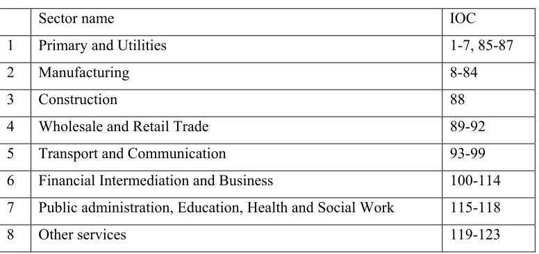
Sectoral aggregation

When we calculate the Rest of the UK matrices, we calculate the Rest of the UK values often as the residual from the UK national IO table minus the values for Scotland and Wales. It is important to ensure that each of the single-region tables is constructed in such a way as making each region consistent with the other. To allow this we aggregated the single-region models in each case to an eight-sector aggregation. This aggregation is shown in Table 3.

This process provided us with a balanced three-region model of the economic linkages between production sectors and final demand categories in Scotland, Wales and the Rest of the UK. In Section III we extend the IO database into a Social Accounting Matrix, and then in Section IV we use these IO and SAM data to examine multiplier values and perform some attribution analysis.

III. Constructing the three-region Social Accounting Matrix (SAM)

SAM and then outline how we have extended the three-region IO table with further information on income transfers to construct a three-region SAM for the UK.

A SAM is a particular representation of the macro and meso economic accounts of a socio-economic system, which captures the transactions and transfers between all economic agents in the system (McGregor et al, 2004a,b; Pyatt and Round, 1985; Reinert and Roland-Holst, 1997). In common with other economic accounting systems, such as IO, the SAM records transactions taking place during a particular accounting period, usually one year. This also means that SAMs are typically build around an Input-Output table (or inter-regional IO table), where the (unchanged) IO table records the transactions between production sectors in the economic system. The main features of a SAM are as follows.

First, the accounts are represented as a matrix, where the incomings and outgoings for each account are shown as a row and corresponding column of the matrix. The transactions are shown in the cells, so the matrix displays the interconnections between agents in an explicit way. Second, the SAM is comprehensive, in the sense that it portrays all the economic activities of the system (production, consumption, accumulation and distribution), although not necessarily in equivalent detail. Thirdly, the SAM is flexible (Thorbecke, 2001), in that, although it is usually set up in a standard basic framework, there is a large measure of flexibility both in the degree of disaggregation and in the emphasis place on different parts of the economic system.

The schematic structure of the three-region SAM is given in Tables 4. There

are four steps, involving different types of data and procedures, which we have used

in its construction.

Type of data used to complete inter-regional SAM table

Shading

1 Data directly available from the existing thee-region IO model as

shown in Table 2

2 Matrices that can be completed from the income-expenditure

accounts constructed for standalone SAMs for Scotland, Wales and

the UK as a whole

3

The disaggregation of net commodity taxes between regions

4

The estimation of other inter-regional transfers

Step 1: Data available from the existing three-region IO model as shown in Table 2.

Step 1.1: Matrices directly from the inter-regional IO table

Some of the matrices in the SAM come directly from the inter-regional IO table as given in Table 2. These are:

Payments from production sectors to production sectors

The matrices showing production linkages between the eight production sectors of Scotland, Wales and the RUK can be read directly from the inter-regional IO table. From this table, we were able to obtain not only each region’s domestic matrices XSS, X

W

W and

XRUKRUK, but also the inter-regional trade matrices XWS, XRUKS, XSW, XRUKW, XSRUK and

XWRUK.

The matrices showing expenditure by production sectors to the Rest of the World (ROW) can be read directly from the inter-regional IO table. The matrices are XROWS, X

ROW W

and XROWRUK,

Rest of the World to Production sectors

The matrices showing expenditure by the Rest of the World on production sectors output can also be read from the IO table for three-regions. This provides the matrices

CSROW, C W

ROWand C RUK

ROW,

Rest of the World to Rest of the World

There are some export expenditures that are directly met by imports. These are given as the scalar CRUKROW,.

Total production sector output and income

The vectors of total outputs of production sectors, TQS, T Q

W, and T Q

RUK can be read

directly from the interregional IO table.

Step 1.2: Matrices from the IO table that are separated out in the SAM

These are matrices that are given in Table 2 that need to be divided up for the

SAM, but where the information is unchanged.

Institutions and Capital to Production

Payments by institutions and capital to production sectors are identified in the inter-regional IO table as CS

S, CWW, CRUKRUK, CWS, CRUKS, CSW, CRUKW, CSRUK and CWRUK. In the

SAM, we need to separate out those demands from institutions, that is Households and Government (there are no direct demands from Net Production Taxes or Corporations) from the demands from the Capital account (investment). These are separately identified here using an I superscript for institutions and a K superscript for the capital account. This means that where Institutions in one region purchase the output of Production in that region, the matrices are given as CI,SS, CI,WW, CI,RUKRUK, while each region’s institutions’ purchases from other

regions’ production sectors are shown in CI,WS, C I,RUK

S, C I,S

W, C I,RUK

W, C I,S

RUK and C I,W

For the purposes of our SAM we have aggregated the GDFCF and Change in Inventories values from the inter-regional IO table into a single “Capital” column for each region. This provides us with the purchases of outputs of production sectors by capital in each region, including inter-regional purchases, and allows us to obtain the matrices CK,SS,

CK,WW, C K,RUK

RUK, C K,W

S, C K,RUK

S, C K,S

W, C K,RUK

W, C K,S

RUK and C K,W

RUK .

Production sectors to Factors of Production

In the three-region IO table, matrices XP

S, XPW, and XPRUK show payments from

Production Sectors to Factors of Production. .Again for the SAM these matrices need to be

disaggregated. The payment to labour and capital is given in matrices XF,SS, XF,WW and

XF,RUKRUK,. Note that production sectors in Scotland (or Wales or RUK) pay factors of

production from Scotland (or Wales of RUK) respectively. There are no inter-regional expenditures in this block, thus there are zero matrices off the diagonal in this payments from production sectors to factors of production block.

Capital to Rest of the World

Within the three-region IO table, payments from the Institutions and Capital accounts of Scotland, Wales and the Rest of the UK to the Rest of the World are given as CROW

S,

CROW

W, and CROWRUK. In the SAM these need to be disaggregated. For the Capital account, the

appropriate matrices are identified as CK,ROWS, CK,ROWW, and CK,ROWRUK.

T

otal expenditure by the capital sector

In the Input-Output table data are given as part of final demand for

expenditure by the capital sector, that is to say, investment. This is part of the vectors

TD

S, TDW, and TDRUK,

. The scalars for total expenditure are extracted from these vectors

and given as

W, and T K

RUK

in Table 4.

Total factor income and expenditure

Again, from the Input-Output Table 2 we can disaggregate those elements of income

from the primary input matrices XP

gives the factor of production income and expenditure total vectors

T

F

W, and

TFRUK

in Table 4.

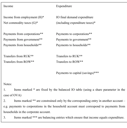
Step 2: Matrices in the inter-regional SAM from single-regional income-expenditure accounts

Since we have identified the sources of all the information necessary for our inter-regional SAM that can be read directly from the inter-inter-regional IO table, the next step is to identify the information that can be obtained from income-expenditure accounts. We use the income-expenditure method (Turner, 2002), to estimate most of the remaining data necessary for the inter-regional Social Accounting Matrix. One of the characteristics of this approach is that it embodies double-entry bookkeeping, in that any item of expenditure in one account (a column entry) simultaneously appears as an item of income in another (a row entry). By constructing single region income-expenditure accounts observing this rule it is possible to fulfil much of the additional data requirements and automatically balance the SAM. For the purposes of our inter-regional SAM data requirements we have five income-expenditure accounts to construct. These are made up of three local transactors – households, government and corporations – the external account (defined as the Rest of the UK and Rest of the World in the income-expenditure accounts for Scotland and Wales, and the Rest of the World in the income-expenditure accounts for the UK), and the capital account.

The format used to construct the income-expenditure accounts can be seen in Table 5. As an example of how the income-expenditure accounts were constructed, detailed notes on the sources and methods used for the income-expenditure account for Wales in 1999 can be found in Appendix 1. Using similar methods, income-expenditure accounts for Scotland and the UK were constructed. Having constructed the income-expenditure accounts for Scotland, Wales and the UK, we could now use this information to complete the inter-regional SAM for the UK.

Factors of production payments to Institutions

income-expenditure accounts obtained for Scotland and Wales. These are shown as matrices FTSS,

FTWW, and FT RUK

RUK.

We note that there are no inter-regional transfers in this matrix, such as between factors of production in Scotland and institutions in Wales. All transfers in this block are assumed to be intra-regional. For the intra-RUK transfers, we again use the income-expenditure accounts constructed for the UK national economy and take the RUK-RUK entries as the residual after subtracting the corresponding Scottish and Welsh entries from each UK one.

Diagonal elements in Institutions to Institutions matrices

In the payments from Institutions to Institutions matrix in Table 4, we can complete the elements of this matrix that record Institutions’ intra-regional transfers to other Institutions. Due to the way in which income-expenditure accounts are constructed there are no payments made by the Scottish household account, for instance, to the Scottish household account, rather any income or expenditure for the household account will come from, or go to, the other institutions. Thus, the elements in the matrices showing payments from Scottish (Welsh) institutions to other Scottish (Welsh) institutions can be read directly from the Scottish (Welsh) income-expenditure accounts. Once again, the RUK values for payments between RUK institutions is found as the residual after subtracting payments from Scottish to Scottish and Welsh to Welsh institutions from total UK intra-agent payments. These are given as matrices ITSS, ITWW, and ITRUKRUK in Table 4.

Payments from the Rest of the World to Institutions and Capital

The transfer of income entries in the inter-regional SAM to and from the Rest of the World can be obtained from the Scottish, Welsh and the Rest of the UK income-expenditure accounts. In the case of Scotland (or Wales) these can be read directly from the Scottish (Welsh) expenditure accounts. For the RUK, these are equal to the UK income-expenditure account entries for each institutions income from the Rest of the World minus the Scottish and Welsh values. These give the matrices ITSROW, IT

W

ROW, IT RUK

ROW, CT S

ROW,

CTWROW, CT RUK

ROW , CT ROW

S, CT ROW

W, and IT ROW

RUK .

Total institutional income and expenditure

These are derived from the standalone regional income-expenditure accounts

and form the matrices

I

W, and T I

RUK.

Total Rest of the World Income and Expenditure

This scalar TIRUKis derived from the income and expenditure accounts

Step 3: The disaggregation of net commodity taxes between regions

P

As explained under Step 1.2 above, we need to split the single net product and production tax row from the matrices XP

S, XPW, and XPRUK in the 3-region IO table. This

allows taxes paid on goods and services imported from other UK regions to be recorded as going to the net commodity tax and government accounts in the exporting region. This provided us with the information that was necessary for the inter-regional SAM on the expenditure by production sectors from Scotland, Wales and RUK to the Net Commodity Accounts of Scotland, Wales and RUK. These payments were recorded in the Net Commodity Tax institution account of the region to which the tax was paid. This gives the matrices XI,SS, X

I,W

W, and X I,RUK

RUK, and also the inter-regional tax flow matrices X I,W

S,

XI,RUKS, XI,SW, XI,RUKW, XI,SRUKand XI,WRUK.

Similarly, the payments of commodity tax by the capital account of each region needed to be separated out from the single row vector identified in the inter-regional IO table. As with the production sectors payments to net commodity taxes in each region, the capital accounts payments to commodity taxes were estimated in the same method. This generates the matrices KTSS, KTWW, KTRUKRUK, KTWS, KTRUKS, KTSW, KTRUKW, KTSRUK

and KTWRUK.

Step 4: Matrices in inter-regional SAM unable to be derived from IO or single-region

income-expenditure accounts

These payments need to be disaggregated into transfers to Wales and RUK in the Scottish case, and Scotland and RUK in the Welsh case.

Inter-regional Institutional transfers

The remaining matrices are those that show the inter-regional income transfers between the institutions of Scotland, Wales and RUK. As previously noted, the income-expenditure account approach had external accounts for Scotland and Wales which contained transfers to the Rest of the UK and the Rest of the World. The values showing transfers outwith the region but within the nation need to be disaggregated between Wales and RUK (for Scotland) and Scotland and RUK (for Wales). Note that we only split the RUK transfer entries in the case of the household and corporate accounts. In the case of inter-governmental transfers (all inter-regional transfers, except capital, are assumed to be intra-agent flows, e.g. Scottish households to Welsh households or Welsh corporations to Scottish corporations), we assume that these will be between the devolved administrations of Scotland and Wales and central government located in the Rest of the UK.

The interregional transfers in the household accounts for Scotland and Wales were split between Wales/RUK and Scotland/RUK respectively based on the expenditure entries in the Scottish and Welsh accounts, which are estimates of transfers of wage income. Therefore, we calculate the income from Scotland and Wales to the Welsh and Scottish income accounts respectively based on the share of RUK wage income that is generated in Scotland and Wales. To split the RUK transfers from Scotland and Welsh corporations we use the regional shares in the generation of other value added. This generates the matrices ITWS, ITRUKS, ITSW, ITRUKW, ITSRUKand ITWRUK.

Institutions payments to capital

The values for each region’s institutions payments to capital were estimate as is explained in Allan et al (2004). Positive income transfers from any one region to the capital account of another are not allocated as capital-to-capital intra-agent transfers. Instead they are reallocated from the own-region capital account entries for households, government and corporations based on the distribution of savings across these transactors in the income-expenditure account of the home-region. This generates the matrices CTSS, CT

W W,

CTRUKRUK, CT W

S, CT RUK

S, CT S

W, CT RUK

W, CT S

RUK and CT W

RUK.

Having constructed the full matrix showing the inter-regional transfers between institutions in Scotland, Wales and the Rest of the UK, this completes the necessary matrices for an inter-regional Social Accounting Matrix. This SAM reveals not only the production linkages between Scotland, Wales and the Rest of the UK, which is shown in the inter-regional IO table, but also the linkages between factors of production, institutions and capital accounts in each of these three regions. The final SAM is presented in Table 6, which has been aggregated from eight to three sectors to conserve space.

In the next section we use models based both on our three-region IO and SAM to examine the economic linkages between Scotland, Wales and the Rest of the UK. We use both multiplier analysis and multiplier methods to attribute output, value added and employment to final demands across the regions of the United Kingdom.

IV: Results from three-region IO and SAM models

The results initially presented here are derived from our 3-region, 8-sector Input-Output (IO) and SAM accounting system for the UK. The three regions are Scotland, Wales and the Rest of the UK (RUK). We discuss the results from our corresponding UK 4-region sets of accounts (whose regional disaggregation is Scotland, Wales, Northern Ireland and England) in Section V, though data constraints limit these accounts to three production sectors.

The inter-regional accounts can be used to derive a model of the UK economy that allows us to examine the spatial and sectoral impact of an exogenous final demand shock in a particular sector in a particular region in the absence of any supply constraints. The effect on each individual region and the country as a whole can therefore be recorded. The inter-regional model is an extension of the single region IO so it is useful to begin by outlining single-region IO multipliers for Scotland, Wales and the UK for 1999. It is then a simple conceptual step to extend this technique to the multi-region model.

4.1 IO Output Multipliers in a Single Region Model

One of the strengths of IO is its ability to model the ultimate impact of marginal changes in final demand. With the necessary caveats regarding fixed technical coefficients and no supply constraints, IO is an extremely useful tool for analysing exogenous final demand shocks. While impact analysis uses the Leontief inverse, (I-A)-1_{, and final demand}

Miller and Blair (1985, p101) describe input-output multipliers as “summary measures” for impact analysis, where final demand changes drive changes in economic activity through the interdependencies of the Leontief inverse. We will also use the multiplier values to indicate the degree of interdependence between industrial sectors and regions within the UK.

As Miller and Blair (1985, p102) note, “the issue of multipliers rests upon the difference between the initial effect of an exogenous (final demand) change and the total effects of that change”. There are two main types of multiplier. A Type I multiplier quantifies the direct and indirect effects of a change in exogenous final demand. The indirect effects are the increased intermediate inputs required directly or indirectly to produce the change in final demand. Type II multipliers identify the direct, indirect and induced effects3_{. With Type II}

multipliers, the input-output system is closed with respect to households, so changes in expenditure by workers employed in the sectors experiencing the exogenous demand change are included. The changes in expenditure of these workers are induced by the expansion in demand for the products and the increase in the wages paid in that sector.

The key element in IO analysis is the Leontief Inverse matrix which shows how much of each industry's output is needed, in terms of direct and indirect requirements, to meet one unit of final demand for a given industry's output (Alexander and Whyte, 1994). Using the Leontief Inverse allows us to show how final demand drives total output:

(4.1)

X

= −

(

I

A

)

Y

where X is the nx1 vector of industry total gross outputs, (I-A)-1 _{is the nxn Leontief Inverse}

matrix, and Y is the nxz vector of total final demands, and there are n industrial sectors and z categories of final demand.

The Leontief Inverse matrix, however, serves a further purpose. This matrix can be written in extended form as:

(4.2)

(

I

A

)

z

z

z

z

z

z

z

z

z

n

n

n n nn

−

=

L

N

MM

MM

O

Q

PP

PP

11 12 1

21 22 2

1 2

L

L

M

M

M

M

L

Each element (zij) identifies the output supported in sector i by a unit of final demand for the output of sector j. Summing down each column ∑zij for production sector j gives the

total output supported in the economy by one unit of final demand for that sector - the output multiplier. Table 7 shows, for illustrative purposes, the conventional Type I Leontief inverse values for Scotland treated as a stand-alone region.

Taking the Primary & Utilities sector as an example, each £1 of final demand supports £1.188 of output in that sector. The original £1 is the direct effect, while the additional 18.8p is the indirect effect. This £1 of demand also creates output in other sectors, leading to an overall Type I multiplier of 1.741. In other words, each £1 of final demand supports an additional 74p of output in the Scottish economy.

Similarly, Type II output multipliers are calculated by summing down the production sector entries in the columns of the Type II Leontief Inverse, where households have been endogenised. Repeating this process for each region, we derive a set of output multipliers as shown in Table 8.

As we expect, the Type II multiplier values are larger than Type I. This is due to the additional activity attributed to the increased consumption demand for goods and services coming from additional wage payments. Also the relative sizes of multiplier values across regions shown in Table 8 are as we would generally expect. In almost all sectors, the multiplier values for RUK are greater than those for Scotland, which in turn are greater than those for Wales4_{. Larger geographical areas, such as the RUK economy (England plus}

Northern Ireland here), will source a greater share of the intermediate and consumption demands from within their own geographic boundaries. Hence there are fewer leakages than smaller economies that rely on trade for a greater share of intermediate inputs.

Employment and Value Added Multipliers in a Single Region Model

In addition to output multipliers, it is also possible to calculate a number of other measures to summarise the impact of an external final demand shocks. These include

employment and value added (VA) multipliers, which show the employment/VA supported in the economy by each unit of final demand. The VA in any sector is calculated as the sum of the Compensation of Employees and Gross Operating Surplus rows in the IO table, thus providing a measure of sectoral GDP.

The calculation of employment or VA multipliers involves generating a coefficient vector showing the corresponding employment or VA associated with each unit of sectoral output. Using employment as an example, the ith element of the vector e is given by:

(4.3) i

i i

E

e

X

=

where Ei is employment in industry. If we construct a nxn diagonal matrix, Φ, where the ith

diagonal element is ei, and all off-diagonal elements are zero, then pre-multiply by the

Leontief inverse, we can derive an nxn employment inverse, Γ:

(4.4)

₍

₎

I

A

Γ = Φ −

where each element, εij, is given by:

(4.5)

ε

=

z e

It is then possible to attribute employment to different final demand categories through the equation:

(4.6)

E

= Γ

Y

where E is the nx1 column vector of sectoral employment levels. Analogous to output multipliers, by summing down each column of the employment inverse the total employment supported by each unit of output for a particular production sector can be found.

Additional to calculating the employment and value added output multipliers, it is

directly generating the final demand. Each element of the resulting matrix, Λ, is the employment supported by a unit increase in direct employment associated with final demand for a particular sector's output. In matrix form this is given as:

(4.7)

Λ = Φ −

(

I

A

)

Φ

where each element, λij, is given by:

(4.8) ij i

ij j

z e

e

λ

=

Three-region Output Multipliers

Using the three-region IO model we have developed for Scotland, Wales and the Rest of the UK, we can analyse the inter-regional spillover effects of output changes in addition to the impact within the region. Equation 4.1 above shows the matrix algebra required to attribute output to final demands, while a similar process can be followed for employment and value added attribution. The major alteration required for multi-region analysis is the introduction of partitioned matrices. The partitioned A-matrix for the three-region model can be illustrated as:

(4.9)

11 12 13

21 22 23

31 32 33

A A A

A A A A

A A A

⎡ ⎤

⎢ ⎥

= ⎢ ⎥

⎢ ⎥

⎣ ⎦

In Equation (4.9) each element is itself a matrix given by Aij where subscript i refers

to the producing region and subscript j to the consuming region. Thus A11, A22 and A33 are the

domestic A matrices for Scotland, Wales and RUK respectively, while all other matrices are trade matrices5_.

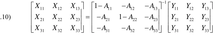
By applying the same process to the other matrices, equation (4.1) can be restated in multi-region format as:

(4.10)

1

11 12 13 11 12 13 11 12 13

21 22 23 21 22 23 21 22 23

31 32 33 31 32 33 31 32 33

1

1

X

X

X

A

A

A

Y

Y

Y

X

X

X

A

A

A

Y

Y

Y

X

X

X

A

A

A

Y

Y

Y

−

−

−

−

⎡

⎤ ⎡

⎤ ⎡

⎢

⎥ ⎢

_{= −}

₋

₋

⎥ ⎢

⎢

⎥ ⎢

⎥ ⎢

⎢

⎥ ⎢

−

−

−

⎥ ⎢

⎣

⎦ ⎣

⎦ ⎣

⎤

⎥

⎥

⎥⎦

In this case, X11 shows the output supported in Region 1 (Scotland) by final demand

in Region 1, X12 shows the output supported in Region 1 by final demand in Region 2 etc.

Similarly, where there are n (8) sectors in each region, the 3nx3n (24x24) Leontief Inverse matrix breaks down the output multiplier for each sector i in each region into local output and imports required per unit of final demand for that sector. The 8x8 sub-matrices (1 - A11), (1 -

A22) and (1 - A33) measure the impact on each of the regions of changes in exogenous demand

in the same region. The column totals from these sub-matrices therefore give the intra-regional impact of final demand shocks, while the other sub-matrices show the impact of trade between regions - the inter-regional effect.

Table 9 shows a summary of Type I and Type II IO output multipliers for each of the three regions. These tables are split into a number of sections, with the first three columns showing the intra-regional impact of an exogenous demand shock. For example, reading down the Scotland column, the Primary & Utilities multiplier is 1.746. Thus, for every £1 of exogenous demand for Primary & Utilities in Scotland, £1.746 of output is supported in Scotland. The equivalent figure for Wales is £1.307, indicating that each £1 of demand for Welsh Primary & Utilities output supports an additional £0.307 of output in Wales.

It is interesting to compare these values to the equivalent single region values shown in Table 8. As can be seen, the regional multipliers are consistently higher, as the intra-regional multipliers include the impact of inter-intra-regional feedback. For instance, given a demand shock, Scottish manufacturers will source some portion of their increased inputs from firms outwith Scotland, which will be included in the inter-regional multipliers. In turn, these firms will obtain some of their increased inputs from Scottish companies and it is this feedback mechanism that causes the intra-regional multipliers to be slightly larger than their single region counterparts.

multipliers than, for example, Wholesale and Retail Trade. This implies that a shock to the Construction sector will have a larger overall impact in the economy that the same magnitude of shock to the Wholesale and Retail Trade sector. It is also interesting to note the large induced effect (difference between Type II and Type I multiplier values) in certain sectors, most notably Public Administration, Health & Social Work and Other Services, indicative of the fact that this sector is highly labour-intensive.

Perhaps most interesting, however, is the pattern of trade between the three regions, represented in the three sections to the right of the intra-regional multipliers in Table 9. The second section shows the multiplier impact of Scottish demand shocks on output in Wales and RUK, giving a measure of trade between the regions. The most obvious trend to note is that Scotland has far stronger linkages to RUK than to Wales. For example, in the Manufacturing sector, the Type I impact of a demand shock in Scotland is to increase Welsh output by £0.024 and RUK output by £0.451. The effect is even more pronounced for a shock in Wales, with the multiplier effect being bigger for RUK than for Wales itself in many cases. On the other hand, the multipliers for RUK trade with Scotland and Wales are very small, reflecting the fact that smaller economic areas often have a greater reliance on trade for inputs to production.

The separate section to the right of the main table shows the total impact throughout the UK of a shock in a particular region. Each figure is calculated by adding the intra- and inter-regional impacts of a change in demand. It is interesting to note that, in contrast to the single region case in Table 8, Scotland now tends to have the largest multiplier values, with RUK now having the smallest multipliers in certain sectors such as Manufacturing and Public Administration, Education, Health & Social Work. However, Welsh multipliers demonstrate the largest percentage change between single- and multi-region multipliers, reflecting the fact that small regions are generally more reliant on external trade than big regions.

Perhaps more interesting, though, is the role of demand from the Rest of the World (ROW) in supporting output. ROW exports account for around 20% of Welsh output, 23% of RUK output and 27% of Scottish output. Thus, Scotland is most reliant on overseas exports to support the economy. This means, however, that Scotland is most susceptible to changes in foreign tastes, exchange rate fluctuations etc. that could impact strongly upon the economy.

Multi-Region Employment and Value Added Multipliers

The calculation of multi-region employment and value added multipliers requires a process similar to that described above for the single region case. Again, we use employment as an example and begin by constructing the inter-regional employment output multiplier matrix, ΓR. This requires, in addition to the output multiplier matrix, a diagonal matrix of

employment/output coefficients. Using these, we can define a 3nx3n (24x24) partitioned matrix of employment/output multipliers as:

(4.11)

1

1 11 12

2 21 22

3 31 32 33

0

0

1

0

0

1

0

0

_

1

R

A

A

A

A

A

A

A

A

A

13 23

−

Φ

−

−

−

⎡

⎤ ⎡

⎢

⎥ ⎢

Γ =

_⎢

Φ

_{⎥ ⎢}

−

−

−

⎢

Φ

⎥ ⎢

−

−

⎣

⎦ ⎣

⎤

⎥

⎥

⎥⎦

where Φi is the diagonal matrix of employment output coefficients for region i.

Thus, we can attribute total employment in the economy to particular sources of final demand through the expression:

(4.12)

11 12 13 11 12 13

21 22 23 21 22 23

31 32 33 31 32 33

R

E E E Y Y Y

E E E Y Y Y

E E E Y Y Y

⎡ ⎤ ⎡

⎢ ⎥_{= Γ} ⎢

⎢ ⎥ ⎢

⎢ ⎥ ⎢

⎣ ⎦ ⎣

where E11 is an nxI matrix showing the employment generated in Region 1 (Scotland) by

production activities in Region 1 to support Region 1 final demand.

Again the multiplier matrix can be expressed in terms of

the employment or value

regional sector directly generating the final demand producing the matrix ΛR. In matrix form

this is given as:

(4.13)

1 1

1 11 12 13 1

2 21 22 23 2

3 31 32 33 3

0

0

1

0

0

0

0

1

0

0

0

0

_

1

0

0

R

A

A

A

A

A

A

A

A

A

− −

Φ

−

−

−

Φ

⎡

⎤ ⎡

⎤ ⎡

⎤

⎢

⎥ ⎢

⎥ ⎢

⎥

Λ =

_⎢

Φ

_{⎥ ⎢}

−

−

−

_{⎥ ⎢}

Φ

_⎥

⎢

Φ

⎥ ⎢

−

−

⎥ ⎢

Φ

⎥

⎣

⎦ ⎣

⎦ ⎣

⎦

Tables 11 and 12 show summaries of employment and value added (VA) multipliers respectively, set out in the same way as the output multipliers described in the previous section. As in the single-region case, these multipliers show the Type I/Type II employment/VA increase in each region associated with a change in final demand for a particular sector's output generating a unit of direct employment or value added.

While the multiplier values are largely in the same order for each region, Financial Intermediation and Business Services differs substantially. This sector has only the 5th largest Type I employment multiplier for Scotland and Wales but the 2nd largest for RUK (largest in Type II). This is probably caused by the concentration of financial services firms in London and the South-East of England and these firms are generally highly labour-intensive. Given that RUK also includes Northern Ireland, the English employment multiplier may be even higher. Furthermore, Financial Intermediation and Business Services has the highest output of any RUK sector and the second highest output in Scotland, implying the sector is a hugely important employer for these regions.

The Construction sector has, quite clearly, the highest VA multipliers in both Scotland and RUK. This is probably due to the fact that this sector is "sheltered" and buys the majority of its inputs from local suppliers. Looking at the intra-regional component would appear to back up this suggestion, with Construction having very large intra-regional multipliers in Scotland and RUK. Although overall in Wales this sector does not have the largest multiplier, the intra-regional component is the biggest, again reinforcing the argument that construction sources its inputs locally. It is also interesting that the Construction sector has a large induced effect, suggesting that it is labour-intensive and/or its sources of supply are labour-intensive.

a significant impact on employment throughout the economy by adjusting their spending levels. It is also worth noting that, while Scotland and RUK both have around 21% of their employment supported by ROW exports, the equivalent value for Wales is just 16%. Thus, in employment terms, Wales should be the most resistant to poor exchange rates etc.

As explained earlier, Value Added (VA) gives a measure of GDP in each region. Table 14 shows the attribution for VA in our inter-regional model. We can see that households from outwith the region support almost half as much VA as do home-region households in both Scotland and Wales. This compares to around a third for the equivalent figure for RUK. Again, this tends to support the view that small geographic regions rely more on external trade than do large regions.

Using the Inter-Regional Social Accounting Matrix

We can also use the three-region Social Accounting Matrix constructed in Section III, to examine the inter-linkages between Scotland, Wales and the Rest of the UK. As with the results presented using the inter-regional IO table, our initial results use the inter-regional SAM to examine multiplier values for output, value added and employment, while also examining output, value added and employment which can be attributable to final demand categories in Scotland, Wales and the Rest of the UK. We calculate Type 2 values for the multipliers in each case, where the household account is made endogenous to the SAM model – the government, capital and Rest of the World account remains exogenous, as in the IO Type 2 case.

SAM Type II multipliers for Output, Employment and Value Added are shown in Table 15, while the attribution of Output, Employment and Value Added to final demand categories across the three regions is shown in Table 16.

V: Incorporating Northern Ireland to construct a four-region Input Output and SAM model of the UK

using these four-region models. For more details on the construction of the four-region IO and SAM models see Allan et al (2004).

Construction of single-region IO table for Northern Ireland

Our initial needs for a four-region model of the UK – involving Scotland, Wales, Northern Ireland and England – were determined by the capacity of AMOSUK, our inter-regional Computable General Equilibrium model (Ferguson et al, 2004). The AMOSUK model uses the SAM data as a key input. Given both the modelling needs and data limitations, we have restricted ourselves in the first instance to a 3-sector, 4-region Input-Output tables The sectors chosen corresponded to IOC classification of production activities, as shown in Table 17.

Therefore our first step was to aggregate the three-region IO and SAM calculated in Sections II and III to these three-sectors. We next estimated the single-region IO table for Northern Ireland, given the lack of official published tables. Our approach was, wherever possible, to use Northern Ireland-specific published data as control totals for individual rows and columns. Then for the column coefficients we used the coefficients from the aggregated three-sector model for Wales. Wales is a similar sized economy to Northern Ireland and we felt would provide an indication of the linkages between Northern Ireland and the rest of the UK. We then used a balancing program to construct the single-region Northern Ireland IO table. This table could then be used as an element in the four-region IO table. However, as with the IO tables of Scotland and Wales, disaggregation of imports from and exports to the Rest of the UK was necessary.

We are aware that Northern Ireland, like Wales, shares a border with a larger economic region – the Rest of the UK (specifically England) in the case of Wales, the Republic of Ireland in the case of Northern Ireland. The differences here is that imports and exports between Northern Ireland and the Republic of Ireland are treated as coming from/going to the Rest of the World, while imports and exports for Wales to England come from/go to the Rest of the UK. This is one issue that we have attempted to consider when we obtained the control total data for Northern Ireland.

1999/00-2000/01” which gave estimates for the manufacturing sector around our base year. Estimated exports in manufacturing to the Rest of the UK were £3,248million, while £3,732million of manufacturing was exports to the Rest of the world.

Figures for Scotland showed that manufacturing exports to the Rest of the UK represented 43.79% of all exports to the Rest of the UK, while for exports to the Rest of the world, manufacturing exports represented 75.06% of all exports. Using these shares and the Northern Ireland figures for total manufacturing exports, we estimated that Northern Ireland exports as £7,417.9million to the Rest of the UK and £4,972million to the Rest of the World.

Similar methods were used to obtain control totals for the other final demand categories - Households, General Government, GDFCF and Inventories - as well as primary inputs – imports from RUK and ROW, net production and commodity taxes, compensation of employees and gross operating surplus. Estimates for the total gross inputs for the three sectors in the model of Northern Ireland.

Tables 18, 20, and 22 show the Type I and Type II output, employment and value-added inter-regional I-O and SAM multipliers for the 4-region model. These correspond to Tables 9, 11 and 12 in the three-region case. The own multiplier values for Northern Ireland are relatively high. Although the economy is small, this perhaps reflects its rather isolated status. Tables 19, 21 and 23 show the supported output in the four regions. Again these figures correspond to those given in Tables 10, 13 and 14 for he three region model. The importance of government expenditure in Northern Ireland for supporting output and employment in the province is shown clearly in these figures.

Section VI: Conclusions

In this paper we detail the way in which we have constructed a disaggregated 3 and 4 region set of I-O and SAM accounts for the UK for the year 1999. These accounts indicate the flows of goods, services and income both within and between regions of the UK and also between the regions of the UK and the Rest of the world. These data are of great value in themselves and are also required for more sophisticated, inter-regional multi-sectoral modelling and analysis.

Bibliography

Alexander, J.M. and Whyte, T.R. (1994), “Output, Income and Employment Multipliers for Scotland”, Scottish Economic Bulletin, No. 50, Winter 1994/95

Allan, G.J., McGregor, P.G., Swales, J.K. and Turner, K. (2004) “Construction of a Multi-Sectoral Inter-Regional IO and SAM database for the UK”, Strathclyde Discussion Papers in Economics, 04-22.

Batey, P.W.J. (1985), “Input-Output Models for Regional Demographic-Economic Analysis: Some Structural Comparisons”, Environment and Planning A, 17, p73-99

Bryan, J., Jones, C., Munday, M. and Roberts, A. (2004) “Welsh Input-Output Tables for 2000”, Welsh Economic Research Unit, Cardiff Business School, downloadable at

http://www.weru.org.uk/output.pdf

Clifton-Fearnside, A. (2001), “Regional Accounts 1999: Part 2, Regional Household Sector Income and Individual Consumption Expenditure”, Economic Trends, No. 573, August, 2001, online at

http://www.statistics.gov.uk/articles/economic_trends/Regional_Accounts_1999_part2.pdf

Ferguson, L., Learmonth, D., McGregor, P.G., McLellan, D., Swales, J.K. and Turner, K. (2004), “The National Impact of Regional Policy: Policy Simulation with Labour Market Constraints in a Two-Regional Computable General Equilibrium Model”, Strathclyde Discussion Papers in Economics, 04-20.

HM Treasury (2001), “Public Expenditure, Statistical Analyses 2001-02”, available online at http://www.hm-treasury.gov.uk/media//BCCBC/32.pdf

McGregor, P.G., McLellan, D., Swales, J.K. and Turner, K. (2004a) “Attribution of Pollution Generation to Local Private and Public Demands in a Small Open Economy: Results from a SAM-based Neo-classical Linear Attribution System for Scotland”, Strathclyde Discussion Papers in Economics, 04-08.

Miller, R.E. and Blair, P.D. (1985) Input-Output Analysis: Foundations and Extension, Prentice Hall

National Assembly for Wales (2002) “Digest of Welsh Statistics, 2002”, online at

http://www.wales.gov.uk/keypubstatisticsforwales/content/publication/compendia/2002/dws2 002/dws2002.htm

Pyatt, G and Round, J. I. (eds) (1985) Social Accounting Matrices: A Basis for Planning, The World Bank, Washington, D.C., U.S.A

Reinert, K. A. and D. W. Roland-Holst (1997) ‘Social Accounting Matrices’, J. F. Francois and K. A. Reinert (eds), Applied Methods for Trade Policy Analysis: A Handbook, Cambridge University Press, Cambridge

Round, J. (1995) ‘A SAM for Europe: Social Accounts at the Regional Level Revisited’, in G. Hewing and M. Madden (eds), Social and Demographic Accounting, Cambridge University Press, New York, NY.

Thorbecke, E. (2001) ‘The Social Accounting Matrix: Deterministic or Stochastic Concept?’ Conference Paper, Cornell University.

Appendix 1: Income and Expenditure Accounts for Wales (1999)6

A set of income-expenditure accounts for Wales in 1999 have been constructed to meet all additional data requirements for construction of a Social Accounting Matrix (SAM). Hence, the data necessary for extending the Welsh 1999 Input-Output (IO) table into a SAM would come from within these income and expenditure accounts.

Completion of a set of internally consistent income-expenditure accounts means that the SAM will automatically balance. Balancing is constrained by the fixed IO entries and it is therefore necessary to manually balance the SAM on the basis of the additional entries in the income-expenditure accounts alone.

One of the key characteristics of a SAM is that it is the embodiment of double-entry bookkeeping, in that any item of expenditure in one account (a column entry) must appear as an item of income in another (the corresponding row entry). By constructing the five sets of income-expenditure accounts observing this rule it is possible to fulfil all the additional data requirements and automatically balance the SAM.

In constructing the income-expenditure accounts it is best to begin with the three local transactors – households, government and corporate – for which data are more readily available from existing published data sources. Table 5 in the text provides a detailed outline of the common format used for all three of these accounts.

The Household Account

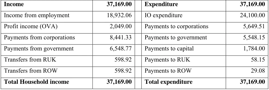
The household account is constructed first, as this account was the one for which information was most readily available. The fixed IO entries in the household income-expenditure account are:

• •

income from employment (from the Welsh IO table) – £18,932.06million

final demand expenditure by households (final consumption from Welsh IO table) – £24,100million

The Household Income and Expenditure account for 1999 is shown in the table below, where all figures are in £millions, 1999 prices).