Bayesian Inference For The Segmented Weibull Distribution

July 2019, Volume 42, Issue 2, pp. 225 to 243 DOI: http://dx.doi.org/10.15446/rce.v42n2.76815

Bayesian Inference for the Segmented Weibull

Distribution

Inferencia bayesiana para distribuciones Weibull segmentadas

Emílio A. Coelho-Barros1,a, Jorge A. Achcar2,b,

Edson Z. Martinez2,c, Nasser Davarzani3,d, Heike I. Grabsch4,e

1

Department of Mathematics, Federal University of Technology, Cornélio Procópio, Brazil

2

Department of Social Medicine, Ribeirão Preto Medical School, University of São Paulo, Ribeirão Preto, Brazil

3

Department of Pathology, GROW School for Oncology and Developmental Biology, Maastricht University Medical Center, Maastricht, The Netherlands 4

Section of Pathology & Tumour Biology, Leeds Institute of Cancer and Pathology, University of Leeds, Leeds, United Kingdom

Abstract

In this paper, we introduce a Bayesian approach for segmented Weibull distributions which could be a good alternative to analyze medical survival data in the presence of censored observations and covariates. With the ob-tained Bayesian estimated change-points we could get an excellent fit of the proposed model to any data sets. With the proposed methodology, it is also possible to identify survival times intervals where a covariate could have significantly different effects when compared to other lifetime intervals, an important point under a clinical view. The obtained Bayesian estimates are obtained using standard Markov Chain Monte Carlo methods. Some exam-ples with real data sets illustrate the proposed methodology and its potential clinical value.

Key words:Bayesian methods; Censored data; Change-points; Covariates; Segmented Weibull distribution.

a_{PhD. E-mail: [email protected]} b_{PhD. E-mail: [email protected]} c_{PhD. E-mail: [email protected]}

Resumen

En este artículo introducimos un nuevo modelo Bayesiano para distribu-ciones Weibull segmentadas, que puede ser una buena alternativa en el análi-sis de datos aplicados a la investigación en salud, con la presencia de cen-suras y covariables. Con este método basado en la estimación de puntos de cambio, hemos obtenido un excelente ajuste a los datos utilizados como ejemplos. De acuerdo con el modelo propuesto, fue posible identificar rangos de valores en las series temporales en que una variable independiente podría tener diferentes efectos. Este es un resultado importante desde el punto de vista clínico. Los estimados bayesianos fueron obtenidos usando métodos de Monte Carlo en Cadenas de Markov. Ejemplos basados en conjuntos de datos reales fueran usados para ilustrar el uso de los modelos propuestos y sus potenciales aplicaciones en investigaciones clínicas.

Palabras clave:Covariables; Datos censurados; Distribución Weibull seg-mentada; Métodos bayesianos; Puntos de cambio.

1. Introduction

In medical research, survival analysis techniques are often used to study time to an event such as death or disease recurrence. A widely used model is based on the Weibull probability distribution function with two parameters for a survival time

T. The Weibull distribution was first described in detail in1951 by the Swedish mathematician Waloddi Weibull (Weibull 1951). Among other advantages of the Weibull distribution, we note that:

• It assumes different shapes due to the flexibility of its hazard rate func-tion (increasing, decreasing or constant depending on the value of its shape parameter);

• It can be seen as a family incorporating other different survival curve shapes, such as the exponential and Rayleigh distributions;

• It can be easily be adjusted for covariates and applied to the regression models;

• Their parameters can be easily estimated (see for example, Pak, Parham & Saraj, 2013; or Kizilaslan & Nadar, 2015).

on cancer incidence where new tumors need time to become detectable while the treatment does not affect pre-existing tumors where there is an approximately two-year waiting period before the effect of the treatment is noticeable. Survival times in these examples have a higher initial failure rate and a lower failure rate afterwards (see other applications in, Goodman, Li & Tiwari 2011; He, Kong & Su 2013; Müller & Wang 1990).

In this case, the literature presents many papers with classical or Bayesian ap-proaches to get inferences for a change-point assuming the exponential distribution which is a special case of the Weibull distribution. In this direction, Matthews & Farewell (1982) considered the problem of testing the hypothesis of the change-point be equal to zero based on the likelihood ratio test statistics and used simu-lations to find the distribution of the statistics of this model with application to medical data related to the treatment of leukemia patients.

Assuming the special case of an exponential distribution, the hazard function in presence of a change-point is given by,

λ(t) =

{

λ ift < ζ

λρ ift≥ζ (1)

whereT >0denotes the lifetime of an individual,λandλρdenote the rates before and after the change-pointζ and the parameterρ >0 denotes the change in the hazard function (a discontinuous change-point).

The probability density function (pdf) for the lifetimeT is given by,

f(t) =

{

λexp (−λt) ift < ζ

λρexp (−λt−λρ(t−ζ)) ift≥ζ (2)

This model approch also could be generalized for situations in presence of a covariate. As a special situation, let us consider a covariate X related to two treatments, that is, each different treatment could lead to different change-points (X= 0 for treatment1andX = 1for treatment2) with hazard function,

λ(t) =

{

λ ift < ζ

λρexp (βx) ift≥ζ (3)

where β is a regression parameter (Achcar & Bolfarine 1989, Achcar & Loibel 1998).

Similarly, assuming a Weibull distribution, the hazard function in presence of a change-point is given by,

λ(t) =

{

λγtγ−1 _{ift < ζ}

λργtργ−1 ift≥ζ (4)

and the pdf is given by,

f(t) =

{

λγtγ−1exp (−λtγ) ift < ζ

Similarly, it is possible to generalize these expressions for the case of two or more change-points (Achcar, Rodrigues & Tzintzun 2011a, Achcar, Rodrigues & Tzintzun 2011b).

Also with a classical inference approach, Matthews, Farewell & Pyke (1985) considered an asymptotic score statistic process to test for constant hazard against a change-point alternative. In another paper, Nguyen, Rogers & Walker (1984) obtained a consistent estimator for the change-point by examining the properties of the density represented as a mixture. Yao (1986) proposed a maximum likeli-hood estimator for the change-point subject to a natural constraint and Worsley (1986) also used maximum likelihood methods to test for a change-point and found the exact null and alternative distributions of the test statistics. Loader (1991) discussed inference based on the likelihood ratio process for a hazard rate change-point and derived approximate confidence regions for the change-change-point.

An approach derived from the Kaplan-Meier estimation of the survival func-tion followed by the least-squares estimafunc-tion for the change-point was introduced by Chen & Baron (2014). Zhao, Wu & Zhou (2009) proposed a change-point model for survival data accounting for long-term survivors with application to the leukemia data analyzed by Matthews & Farewell (1982). Achcar & Bolfarine (1989) presented a Bayesian analysis of the exponential model assuming a change-point as either known or unknown. In another paper, Achcar & Loibel (1998) consid-ered Bayesian inferences for the exponential model assuming change-point using different prior densities. Karasoy & Kadilar (2007) introduced another Bayesian approach for constant hazard functions applied to data of breast cancer patients and some lymphoma data. Assuming a Weibull distribution in presence of a single change-point, Jiwani (2005) introduced a single change-point parametric Weibull model, considering the case where the survival function is subject to a change from a given instant. Yiannoutsos (2009) used the model proposed by Jiwani (2005) to estimate survival among HIV-infected patients who are initiating antiretroviral therapy in sub-Saharan Africa.

In this paper, we introduce a Bayesian inference approach for the segmented Weibull model assuming one or more unknown change-points. For the Bayesian analysis of the model, we use standard existing Markov Chain Monte Carlo (MCMC) methods to simulate samples of the joint posterior distribution of interest. Appli-cations are considered using clinical data sets in presence of change-points with continuous survival function.

2. Methods

LetT denoting a continuous non-negative random variable denoting a lifetime with probability density function (pdf)f(t)and cumulative distribution function (cdf)F(t) =P(T ≤t). Under the assumption of a Weibull distribution, the pdf is given by,

f(t) = α

µαt α−1_exp

[ −

(

t µ

)α]

wheret >0, µ >0 and α >0. The Weibull distribution is characterized by two parametersµandα, whereµis a scale parameter andαis a shape parameter.

The survival function is given by,

S(t) = 1−F(t) = exp

[ −

(

t µ

)α]

. (7)

The hazard function or the instantaneous rate of occurrence is given by,

h(t) = f(t)

S(t)=

α µαt

α−1_{. (8)}

The hazard functionh(t)is increasing ifα >1, decreasing ifα <1 and constant ifα= 1(an exponential distribution).

The mean and variance of the Weibull distribution with density (6)are given respectively by,

E(T) =µΓ

(

1 + 1

α

)

(9)

and,

V ar(T) =µ2

[

Γ

(

1 + 2

α

) −Γ2

(

1 + 1

α

)]

. (10)

The cumulative hazard function is given by,

Λ(t) =

∫ t

0

h(x)dx=

(

t µ

)α

, (11)

that is,

g(t) = ln [Λ(t)] =αln (t)−αln (µ), (12) In this way the survival function is,

S(t) =P(T > t) = exp [−Λ(t)]. (13)

2.1. Presence of One Change-Point

In presence of a change-point a1, we define for the ith observation

(i= 1,2, . . . , n),

g1(ti) =ci[α1ln (ti)−α1ln (µ1)] + (1−ci) [α2ln (ti)−α2ln (µ2)], (14)

where, ci = 1−step(ti−a1), andstep(ti−a1) = 1ifti > a1;step(ti−a1) = 0

if0< ti≤a1.

In this way we have five parameters to be estimated: a1, α1, α2, µ1 andµ2.

The cumulative hazard function in presence of the change-pointa1, is given by,

and the hazard function is given by,

h1(ti) =

dΛ1(ti)

dti

=dg1(ti)

dti

exp [g1(ti)], (16)

where, dg1(ti) dti =

1

ti[ciα1+ (1−ci)α2], that is,

h1(ti) = 1

ti

[ciα1+ (1−ci)α2] exp [g1(ti)], (17)

and,

S1(ti) = exp [−Λ1(ti)] = exp{−exp [g1(ti)]}. (18)

The density function is given, fromf1(ti) =h1(ti)S1(t1), by,

f1(ti) =

1

ti

[ciα1+ (1−ci)α2] exp{g1(ti)−exp [g1(ti)]}. (19)

2.2. Likelihood Function in Presence of Censored

Observations

Let T1, T2, . . . , Tn be a random sample of size n of lifetimes in presence of

censored observations, where the observed times are given by ti = min (Ti, Ci)

(type I censoring) where Ci are the censoring times andi = 1,2, . . . , n; thus we

can define the indicator variable,

δi=

{

1(complete observation)

0(censoring observation). (20)

For theith_{individual, the contribution for the likelihood function is given by,}

Li= [h1(ti)]

δi_{exp [}−_Λ

1(ti)]. (21)

The log-likelihood function assuming only one change-point is given by,

l(θ) = n

∑

i=1

δiln [h1(ti)]− n

∑

i=1

exp [g1(ti)] (22)

where, θ= (a1, α1, α2, µ1, µ2),h1(ti) is given in(17)and g1(ti)is given in (14),

that is,

l(θ) = n

∑

i=1

δiln (ti) + n

∑

i=1

δiln [ciα1+ (1−ci)α2]

+ n

∑

i=1

δig1(ti)− n

∑

i=1

Note 1. For the case of one change-point, when we have the continuity for the survival function in the change-point t = a1, we have: α1ln (a1)−α1ln (µ1) =

α2ln (a1)−α2ln (µ2), that is,

α2ln (µ2) =α2ln (a1)−α1ln (a1) +α1ln (µ1), (24)

or,

µ2= exp [

(α2−α1) ln (a1) +α1ln (µ1)

α2

]

. (25)

2.3. A Bayesian Analysis of the Model Assuming One

Change-Point

For a Bayesian analysis of the Weibull distribution in presence of change-points, we assumeGamma(b1, b2)prior distributions for the shape parametersα1 andα2

and for the scale parameterµ1, whereGamma(b1, b2)denotes a gamma

distribu-tion with mean b1

b2 and variance

b1

b2 2

; the scale parameter µ2 was estimated using

(25). For the change-point a1, we assume a uniform prior distribution on the

interval (0, Tm), where Tm is the maximum value observed in the lifetime data.

Further let us assume prior independence among the parameters.

Combining the joint prior distribution forθ= (a1, α1, α2, µ1, µ2)with the

like-lihood functionL(θ), the posterior distribution forθis determined from the Bayes formula (Box & Tiao 1973). The posterior summaries of interest are obtained us-ing Markov Chain Monte Carlo (MCMC) methods (Gelfand & Smith 1990, Chib & Greenberg 1995). A great simplification in the generation of samples from the posterior distribution forθ is obtained by using the procedure MCMC (SAS In-stitute Inc 2016) from the software SAS (University Edition), which only requires the specification of the distribution for the data and a prior distribution for the parameters of the model.

Under our proposed model approach, it is observed that it is not possible to get explicit forms for the marginal posterior distributions for each parameter. In this way, we could use some approximation method to solve integrals as the Laplace method (Tierney, Kass & Kadane 1989) or some numerical method (Naylor & Smith 1982). An alternative is to use simulation methods like the Markov Chain Monte Carlo methodology (Gelfand & Smith 1990, Hastings 1970) or acceptation-rejection algorithms such as the Adaptive Rejection Sampling (ARS) or the Adap-tive Rejection Metropolis Sampling (ARMS) (Devroye 1986).

Monte Carlo Markov chains are becoming a standard way to simulate posterior summaries of interest that allows us to solve a wide range of problems (Tierney 1994). To simulate samples of the joint posterior distribution of interest, we need the full conditional posterior distribution for each parameter, from where it is used the Gibbs sampling algorithm (see, for example, Gelfand and Smith, 1990) when these conditional distribution are simple to simulate samples.

In this way, we follow the algorithm,

Step 2 Given current estimatesa(₁i),α₁(i),α₂(i),µ(₁i)andµ(₂i)simulate new values:

• a(₁i+1)from π

(

a1|α₁(i), α(₂i), µ(₁i), µ(₂i),t, δ

)

.

• α(₁i+1)fromπ

(

α1|a(₁i+1), α(₂i), µ(₁i), µ(₂i),t, δ

)

.

• α(₂i+1)fromπ

(

α2|a(₁i+1), α(₁i+1), µ(₁i), µ(₂i),t, δ

)

.

• µ(₁i+1)from π

(

µ1|a(₁i+1), α(₁i+1), α(₂i+1), µ(₂i),t, δ

)

.

• µ(₂i+1)from π

(

µ2|a(₁i+1), α(₁i+1), α(₂i+1), µ(₁i+1),t, δ

)

.

Step 3 Return to step 2.

The sequence

(

a₁(i), α(₁i), α₂(i), µ(₁i), µ(₂i)

)

i= 1, . . . , Lis a realization of a Markov

chain which, under mild regular conditions, has an equilibrium distribution

π(a1, α1, α2, µ1, µ2|t, δ), the joint posterior distribution ofa1,α1,α2,µ1andµ2.

However, in the case that the conditional posterior densities for the parame-ters show that standard sampling schemes are not feasible since the conditional distributions are not in a known form, Bayesian inference for the parameters can be obtained using the Metropolis-Hastings algorithm (Chib & Greenberg 1995) considering the conditional distributions as the target densities.

2.4. Presence of More Than One Change-Point

Once a first change-pointa1was estimated (denoted as stage1), we could use

the Bayesian approach to search for a second change-pointa2 based on the

infor-mation that the first change-point is a known quantitya1(the Bayesian estimate

based on a square error loss function of the first change-pointa1):

(1) In this way, we assume a uniform prior distributionU(a1, Tm)for the second

change-point whereTmis the maximum value observed in the lifetime data.

We also assume that for a1 < t < a2 the values of α1 andµ1 are assumed

to be known and equal to the Bayesian estimates for α2 andµ2obtained in

the stage1. This guarantee the continuity of the Weibull segmented survival function.

(2) Once the second change-point is estimated (denoted as stage2), we assume a uniformU(a2, Tm)prior for the third change-point. We also assume that

fora2< t < a3the values ofα1 andµ1are assumed to be known and equal

to the Bayesian estimates forα2andµ2obtained in the stage2. We continue

this procedure until it is not possible to estimate more change-points.

change-point smaller than the first change-point we could assume an uniform

U(0, a1)prior in place of an uniform priorU(a1, Tm)in (1).

3. Applications With Real Data

In this section we present two applications with real data sets. First we con-sider a data set presented in Chapter 2 of the book of Hosmer, Lemeshow & May (2008). The second data was obtained from a trial conducted by the Leeds Teaching Hospitals NHS Trust, England.

3.1. BPD Data Set

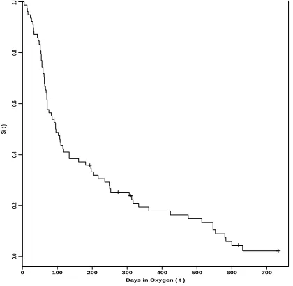
As a first application, we consider a data set (BPD Data) introduced in Chapter

2 of the book of Hosmer et al. (2008). This data set have78 observations and we consider two variables; Days on Oxygen (time to event) and the Censoring Indicator: 1 =Off Oxygen and0 =Still on Oxygen. In Figure 1, we have the plot of the (Kaplan & Meier 1958) nonparametric estimate of the survival function (use of the R software). From this graph we observe the indication of a possible first change-point close to time t = 100 and a possible second change-point close to

t= 500.

0 100 200 300 400 500 600 700

0.0

0.2

0.4

0.6

0.8

1.0

Days in Oxygen ( t )

S( t )

Figure 1: Kaplan Meier estimate for the survival function (BPD data).

For a Bayesian analysis of the model in a first stage, let us assume a Weibull dis-tribution with density(6)in the presence of a change-point and assuming continu-ity of the survival function at the change-point, see(25). AssumingGamma(0.01,

parameterµ1; we consider an uniformU(0,733)prior distribution for the

change-pointa1(first stage of the Bayesian analysis). We have used the procedure MCMC

(SAS Institute Inc 2016) from the software SAS (University Edition), a single chain has been used in the simulation of samples for the parameters considering a “burn-in-sample” of size 10,000 to eliminate the possible effect of the initial values. After this “burn-in” period, we simulated other 500,000 Gibbs samples taking every200thsample, to get approximated uncorrelated values which result in a final chain of size2,500. Convergence of the algorithm was verified from trace plots of the simulated samples for each parameter and usual existing convergence diagnostics available in the literature for a single chain using the SAS/MCMC pro-cedure indicated convergence for all parameters. In Table1, we have the posterior summaries of interest (first segment of the Weibull distribution).

Table 1:Posterior summaries (Weibull with a change-point).

Parameter Mean Standard Deviation 95%Credible Interval

a1 84.60 17.816 (68.40; 125.0)

α1 1.846 0.3669 (1.219; 2.643)

α2 0.739 0.1035 (0.542; 0.941)

µ1 111.2 17.407 (85.65; 151.1)

µ2 166.8 30.332 (111.2; 230.6)

For a second change-pointa2(second stage of the analysis) we assume a uniform

U(84.6,733) prior for a2, α1 = 0.739, µ1 = 166.8 obtained from the first stage,

and the same prior distributions for the other parametersα2 andµ2 considered

in the first stage. Using the same simulation steps used in the estimation of the parameters in the first stage (results in Table 1), we have in Table 2, the posterior summaries of interest (second segment of the Weibull distribution).

Table 2: Posterior summaries (Weibull second change-point).

Parameter Mean Standard Deviation 95%Credible Interval

a2 534.5 75.812 (364.8; 715.0)

α2 2.302 1.1970 (0.743; 5.432)

µ2 348.2 89.793 (166.9; 572.6)

Since the second change-point(a2= 534.5)is a large value close to the lifetime

t = 733 (maximum observed lifetime), we stop the search method looking for new change-points. In this way, the survival function could be splited in three segmented Weibull pieces:

S(t) =

                 exp [ −( t

111.2 )1.846]

if0< t <84.6

exp

[ −( t

166.8 )0.739]

if84.6≤t <534.5

exp

[ −( t

348.2 )2.302]

ift≥534.5

(26)

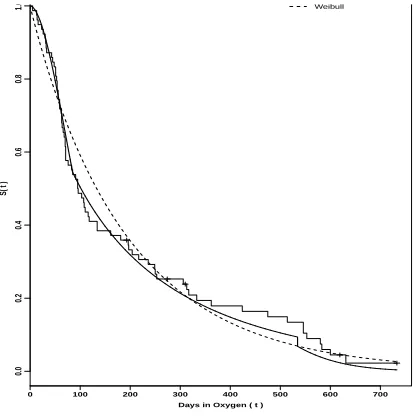
change-points, and also assuming a Weibull distribution not considering the presence of change-points. We clearly observe better fit of the Weibull distribution in the presence of two change-point for the BPD data set.

0 100 200 300 400 500 600 700

0.0

0.2

0.4

0.6

0.8

1.0

Days in Oxygen ( t )

S( t )

Weibull

Figure 2: Bayesian estimates for the survival function (BPD data).

3.2. Leeds Gastric Cancer Series

In second application, we evalue a data set with906 patients who were diag-nosed with gastric cancer and underwent surgery between 1968 and 2009at the Leeds Teaching Hospitals NHS Trust, Leeds, UK. The overall survival time of861

patients is available as time to death or censoring time (in years). Lymph node metastasis status in gastric cancer (pN category) was measured for each patient, werepN = 0, no lymph node metastases; pN = 1, otherwise. The pN category is a very well established prognostic factor of gastric cancer (Deng & Liang 2014) and one might be interested to analyze pN category in terms of survival time of patients.

In this data set there are 861 patients where 222 lifetimes are right censored data. The median follow-up time was1.67years, ranging from0.01to20.56years. First of all, we assume a lifetime regression model (Weibull regression model) for the response (overall survival) in the presence of covariate gender (1: male; 0: female) and pN (pN = 0, no lymph node metastases; pN = 1, otherwise) given by,

ln (ti) =β0+β1genderi+β2pNi+εi, (27)

where,tidenote the overall survival for theithpatient, i= 1, . . . ,861;β0,β1and

quantity with an extreme value distribution (Lawless 2003) with density,

f(ε) = exp [ε−exp (ε)], − ∞< ε <∞, (28)

then we have a Weibull regression model. Other distributions also could be as-sumed for the error. If the error termεiin(27)has a standard normal distribution,

we have a log-normal distribution for the lifetimeT.

Using the procedure MCMC from the software SAS (University Edition), we have in Table 3, the Bayesian estimates of the regression parameters assuming a Weibull distribution with n = 861 observations (639 complete lifetimes and 222

censored lifetimes). We consider normal priors with mean µ = 0 and variance

σ2_{= 10000for the regression parametersβ}

0,β1 andβ2and aGamma(0.01,0.01)

prior for the Weibull shape parameterα. We consider a single chain in the simu-lation of samples for the parameters considering a “burn-in-sample” of size10,000

to eliminate the possible effect of the initial values. After this “burn-in” period, we simulated other500,000Gibbs samples taking every200thsample, to get approxi-mated uncorrelated values which result in a final chain of size2,500. Convergence of the algorithm was verified from trace plots of the simulated samples for each parameter and usual existing convergence diagnostics available in the literature for a single chain using the SAS/MCMC procedure indicated convergence for all parameters.

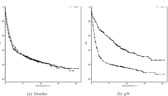
From the results of Table 3, we observe that the covariate gender has not significant effect in the overall survival times (zero is included in 95% credible interval), but the covariate pN presents significative effect on the overall lifetimes of the patients. In Figure3, we have the plots of the Kaplan-Meier nonparametric estimate of the survival functions.

Table 3: Posterior summaries for parameters (Weibull regression model with covariates gender and pN).

Parameter Mean Standard Deviation 95%Credible Interval

β0 2.4404 0.1375 (2.1793; 2.7100)

β1 0.0651 0.1364 (−0.217; 0.3300)

β2 −1.462 0.1523 (−1.767;−1.168)

0 5 10 15 20

0.0

0.2

0.4

0.6

0.8

1.0

Survival time ( t )

S( t )

Male

(a) Gender

0 5 10 15 20

0.0

0.2

0.4

0.6

0.8

1.0

Survival time ( t )

S( t )

pN = 1

(b) pN

Figure 3: Kaplan-Meier estimate for the survival functions (gender and pN).

From the plots of Kaplan-Meier presented in Figure3, we observe that is an indication of a change-point close to the survival time t = 2. In this way, we will assume a segmented Weibull distribution with a change-point considering all data set.

3.2.1. Change-Point for the Survival Function Not Considering the Presence of Covariates

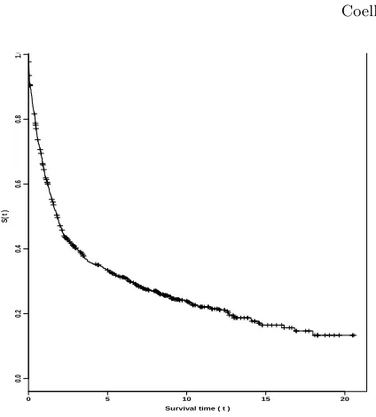
In Figure 4, we have the plot of the Kaplan-Meier nonparametric estimate of the survival functions not considering the presence of covariates. From the graph of Figure 4, we observe a possible change-point close to time t= 2. In this case, we have an indication of only one change-point. For a Bayesian analysis of the model, let us assume a Weibull distribution with density(6)in the presence of a change-point assuming continuity of the survival function at the change-point. Let us assumeGamma(0.01,0.01)prior distributions for the shape parametersα1and

α2 and for the scale parameterµ1 and an uniform U(0,20.56) prior distribution

for the change-point a1 (first stage of the Bayesian analysis). Using the same

0 5 10 15 20

0.0

0.2

0.4

0.6

0.8

1.0

Survival time ( t )

S( t )

Figure 4: Kaplan Meier estimate for the survival function (not considering covariates)

Table 4: Posterior summaries (a change-point segmented Weibull).

Parameter Mean Standard Deviation 95%Credible Interval

a1 2.2609 0.0866 (2.0975; 2.4622)

α1 0.7265 0.0314 (0.6678; 0.7881)

α2 0.3938 0.0267 (0.3422; 0.4467)

µ1 3.0203 0.2096 (2.6443; 3.4693)

µ2 3.8504 0.4119 (3.0841; 4.6985)

In this way, the survival function could be splited in two segmented Weibull pieces:

S(t) =

      

exp

[ −( t

3.0203 )0.7265]

if0< t <2.2609

exp

[ −( t

3.8504 )0.3938]

ift≥2.2609

(29)

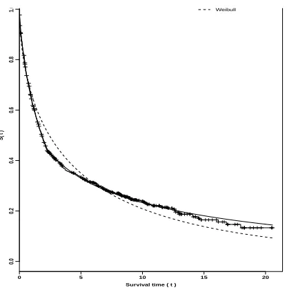
In Figure 5, we have the plots of the Kaplan-Meier survival curve; the esti-mated survival curve assuming a Weibull distribution in the presence of a change-point, and also assuming a Weibull distribution not considering the presence of change-points. We observe an excellent fit of the segmented Weibull distribution considering a change-point for the data.

3.2.2. Effect of the Covariate pN On the Survival Probabilities Considering the Segmented Weibull Distribution

0 5 10 15 20

0.0

0.2

0.4

0.6

0.8

1.0

Survival time ( t )

S( t )

Weibull

Figure 5: Bayesian estimates for the survival function (NHS data).

Tables 5 and 6, it is presented the Bayesian estimates of the regression parameters assuming a Weibull distribution in presence of the covariate pN and the change-pointa1= 2.2609. We consider the same priors and simulation steps used in the

estimation of the parameters in the Weibull regression model (results in Table 3).

Table 5: Posterior summaries for parameters (segmented Weibull regression model with covariate pN and survival<2.2609).

Parameter Mean Standard Deviation 95%Credible Interval

β0 −0.052 0.1071 (−0.254; 0.1624)

βt<2.2609 −0.119 0.1188 (−0.353; 0.1039)

α 0.9898 0.0383 (0.9173; 1.0664)

Table 6: Posterior summaries for parameters (segmented Weibull regression model with covariate pN and survival≥2.2609).

Parameter Mean Standard Deviation 95%Credible Interval

β0 2.7931 0.0836 (2.6384; 2.9630)

βt≥2.2609 −0.287 0.1072 (−0.499;−0.078)

α 1.4816 0.0962 (1.2978; 1.6791)

From Tables 5 and 6, we observe that for survival times less than2.2609years there was no statistical difference between survival of patients with lymph node metastases and patients with no lymph node metastases (zero is included in95%

patients with lymph node metastases are1.53(HR=exp(0.287×1.4816)) times more in the risk of death than patients with no lymph node metastases.

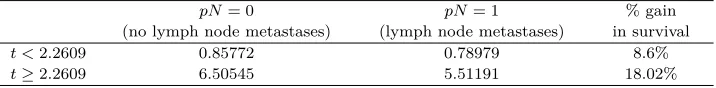
We can also observe the effect of the covariate pN for survival times<2.2609

and survival times≥2.2609considering the uncensored observations by observing the sample means in each case (see Table 7).

Table 7: Sample means for uncensored lifetimes considering the covariate pN assuming a change-point2.2609.

pN = 0

(no lymph node metastases)

pN = 1

(lymph node metastases)

%gain

in survival

t <2.2609 0.85772 0.78979 8.6%

t≥2.2609 6.50545 5.51191 18.02%

4. Concluding Remarks

The use of segmented Weibull distributions could be a good alternative to an-alyze survival times, since with this methodology, we could fit different survival functions and correspondent hazard functions for lifetimes with any hazard func-tion shape. The Bayesian approach introduced in this paper does not require sophisticated computational expertize specially using MCMC simulation methods and the free available software SAS (University Edition).

From the results of this study, we also could get useful interpretations for clinical medical survival data assuming segmented Weibull distributions. Some important points:

• With the use of standard Kaplan-Meier estimation for survival curves it is only possible to compare the survival times together; similarly, if we as-sume Weibull or other parametric lifetime distributions not considering the presence of change-points;

• The use of a segmented Weibull distributions in presence of change-points gives better estimates for the survival curves than using a Weibull distribu-tion without considering the presence of change-points;

• By estimating the change-points, we can compare the survival curves in different intervals which might tell us that the survivals are different in one time interval and not different in another interval, as we have observed in the second application with real data set (Leeds Gastric Cancer Series).

These results can be of great interest in medical applications.

Acknowledgements

[_{Received: December 2018 — Accepted: May 2019}]

References

Achcar, J. A. & Bolfarine, H. (1989), ‘Constant hazard against a change-point alternative: a Bayesian approach with censored data’, Communications in Statistics-Theory and Methods18(10), 3801–3819.

Achcar, J. A. & Loibel, S. (1998), ‘Constant hazard function models with a change point: A Bayesian analysis using Markov chain Monte Carlo methods’, Bio-metrical journal 40(5), 543–555.

Achcar, J. A., Rodrigues, E. R. & Tzintzun, G. (2011a), ‘Modelling interoccurrence times between ozone peaks in Mexico City in the presence of multiple change points’, Brazilian Journal of Probability and Statistics25(2), 183–204.

Achcar, J. A., Rodrigues, E. R. & Tzintzun, G. (2011b), ‘Using non-homogeneous poisson models with multiple change-points to estimate the number of ozone exceedances in Mexico City’,Environmetrics22(1), 1–12.

Box, G. E. P. & Tiao, G. C. (1973), Bayesian inference in statistical analy-sis, Addison-Wesley Publishing Co., Reading, Mass.-London-Don Mills, Ont. Addison-Wesley Series in Behavioral Science: Quantitative Methods.

Chen, X. & Baron, M. (2014), ‘Change-point analysis of survival data with appli-cation in clinical trials’,Open Journal of Statistics4(09), 663–677.

Chib, S. & Greenberg, E. (1995), ‘Understanding the metropolis-hastings algo-rithm’,The American Statistician49(4), 327–335.

Deng, J.-Y. & Liang, H. (2014), ‘Clinical significance of lymph node metastasis in gastric cancer’,World Journal of Gastroenterology20(14), 3967–3975.

Desmond, R. A., Weiss, H. L., Arani, R. B., Soong, S.-j., Wood, M. J., Fid-dian, P. A., Gnann, J. W. & Whitley, R. J. (2002), ‘Clinical applications for change-point analysis of herpes zoster pain’, Journal of pain and symptom management23(6), 510–516.

Devroye, L. (1986), Non-Uniform Random Variate Generation, Springer-Verlag, New York.

Gelfand, A. E. & Smith, A. F. M. (1990), ‘Sampling-based approaches to cal-culating marginal densities’, Journal of the American Statistical Association 85, 398–409.

Hastings, W. K. (1970), ‘Monte Carlo sampling methods using Markov chains and their applications’,Biometrics57, 97–109.

He, P., Kong, G. & Su, Z. (2013), ‘Estimating the survival functions for right-censored and interval-right-censored data with piecewise constant hazard func-tions’,Contemporary clinical trials35(2), 122–127.

Hosmer, D. W., Lemeshow, S. & May, S. (2008),Applied survival analysis: regres-sion modeling of time to event data, Wiley-Interscience.

Jandhyala, V., Fotopoulos, S. & Evaggelopoulos, N. (1999), ‘Change-point meth-ods for weibull models with applications to detection of trends in extreme temperatures’, Environmetrics: The official journal of the International En-vironmetrics Society10(5), 547–564.

Jiwani, S. L. (2005), Parametric changepoint survival model with application to coronary artery bypass graft surgery data, PhD thesis, Statistics and Actu-arial Science department, Simon Fraser University, Canada.

Kaplan, E. L. & Meier, P. (1958), ‘Nonparametric estimation from incomplete observations’,Journal of the American Statistical Association53, 457–481.

Karasoy, D. S. & Kadilar, C. (2007), ‘A new Bayes estimate of the change point in the hazard function’, Computational statistics & data analysis 51(6), 2993– 3001.

Kizilaslan, F. & Nadar, M. (2015), ‘Classical and bayesian estimation of reliabil-ity inmulticomponent stress-strength model based on weibull distribution’,

Revista Colombiana de Estadística 38(2), 467–484.

Lawless, J. F. (2003),Statistical models and methods for lifetime data, Wiley Series in Probability and Statistics, second edn, John Wiley & Sons, Hoboken, NJ.

Loader, C. R. (1991), ‘Inference for a hazard rate change point’, Biometrika 78(4), 749–757.

Matthews, D. E. & Farewell, V. T. (1982), ‘On testing for a constant hazard against a change-point alternative’,Biometrics38(2), 463–468.

Matthews, D., Farewell, V. & Pyke, R. (1985), ‘Asymptotic score-statistic pro-cesses and tests for constant hazard against a change-point alternative’,The Annals of Statistics13(2), 583–591.

Müller, H.-G. & Wang, J.-L. (1990), ‘Nonparametric analysis of changes in hazard rates for censored survival data: An alternative to change-point models’,

Biometrika 77(2), 305–314.

Nguyen, H., Rogers, G. & Walker, E. (1984), ‘Estimation in change-point hazard rate models’, Biometrika71(2), 299–304.

Noura, A. & Read, K. (1990), ‘Proportional hazards changepoint models in sur-vival analysis’, Journal of the Royal Statistical Society: Series C (Applied Statistics) 39(2), 241–253.

Pak, A., Parham, G. A. & Saraj, M. (2013), ‘Inference for the weibull distribution based on fuzzy data’,Revista Colombiana de Estadística36(2), 337–356.

SAS Institute Inc (2016),SAS/STAT⃝R _{14.2 User’s Guide, The MCMC Procedure,}

Cary, NC: SAS Institute Inc.

Sertkaya, D. & Sözer, M. T. (2003), ‘A bayesian approach to the constant haz-ard model with a change point and an application to breast cancer data’,

Hacettepe Journal of Mathematics and Statistics32, 33–41.

Tierney, L. (1994), ‘Markov chains of exploring posterior distributions’,Annals of Statistics 22, 1701–1762.

Tierney, L., Kass, R. E. & Kadane, J. B. (1989), ‘Fully exponential Laplace ap-proximations to expectations and variances of nonpositive functions’,Journal of the American Statistical Association 84(407), 710–716.

Weibull, W. (1951), ‘A statistical distribution function of wide applicability’, Jour-nal of Applied Mechanics18, 293–297.

Whiteley, N., Andrieu, C. & Doucet, A. (2011), ‘Bayesian computational methods for inference in multiple change-points models’. Discussion paper, University of Bristol, UK.

Worsley, K. (1986), ‘Confidence regions and tests for a change-point in a sequence of exponential family random variables’,Biometrika73(1), 91–104.

Yao, Y. C. (1986), ‘Maximum likelihood estimation in hazard rate models with a change-point’, Communications in Statistics-Theory and Methods 15(8), 2455–2466.

Yiannoutsos, C. T. (2009), ‘Modeling aids survival after initiation of antiretroviral treatment by Weibull models with changepoints’,Journal of the International AIDS Society12(1), 1–10.

Zhao, X., Wu, X. & Zhou, X. (2009), ‘A change-point model for survival data with long-term survivors’, Statistica Sinica19, 377–390.

Zucker, D. M. & Lakatos, E. (1990), ‘Weighted log rank type statistics for compar-ing survival curves when there is a time lag in the effectiveness of treatment’,