Computerized adaptive test and decision trees: A unifying approach

This is a repository copy of Computerized adaptive test and decision trees: A unifying

approach.

White Rose Research Online URL for this paper:

http://eprints.whiterose.ac.uk/137468/

Version: Accepted Version

Article:

Delgado-Gómez, D., Laria, J.C. and Ruiz-Hernandez, D. orcid.org/0000-0001-5538-6930

(2019) Computerized adaptive test and decision trees: A unifying approach. Expert

Systems with Applications, 117. pp. 358-366. ISSN 0957-4174

https://doi.org/10.1016/j.eswa.2018.09.052

Article available under the terms of the CC-BY-NC-ND licence

(https://creativecommons.org/licenses/by-nc-nd/4.0/).

Reuse

This article is distributed under the terms of the Creative Commons Attribution-NonCommercial-NoDerivs (CC BY-NC-ND) licence. This licence only allows you to download this work and share it with others as long as you credit the authors, but you can’t change the article in any way or use it commercially. More

information and the full terms of the licence here: https://creativecommons.org/licenses/

Takedown

If you consider content in White Rose Research Online to be in breach of UK law, please notify us by

Computerized adaptive test and decision trees: a

1

unifying approach

2

David Delgado-G´omeza,∗_{, Juan C. Laria}a_{, Diego Ruiz-Hern´andez}b 3

a

Universidad Carlos III de Madrid, Department of Statistics, Legan´es, Spain

4

b

University of Sheffield Management School, Sheffield, UK

5

Abstract 6

In the last few years, several articles have proposed decision trees (DTs) as an alternative to computerized adapted tests (CATs). These works have focused on showing the differences between the two methods with the aim of identifying the advantages of each of them and thus determining when it is preferable to use one method or another. In this article, Tree-CAT, a new technique for building CATs is presented. Unlike the existing work, Tree-CAT exploits the similarities between CATs and DTs. This technique allows the creation of CATs that minimise the mean square error in the estimation of the examinee’s ability level, and controls the item’s exposure rate. The decision tree is sequentially built by means of an innovative algorithmic procedure that selects the items associated with each of the tree branches by solving a linear program. In addition, our work presents further advantages over alternative item selection techniques with exposure control, such as instant item selection or simultaneous administration of the test to an unlimited number of participants. These advantages allow accurate on-line CATs to be implemented even when the item selection method is computationally costly.

Keywords: Decision trees, linear programming, computerized adaptive tests 7

1. Introduction 8

Computerized Adaptive Tests (CATs) are sophisticated tests capable of im-9

proving the accuracy of conventional tests while administering a much smaller 10

number of items (Weiss, 2004). They are based on the Item Response Theory 11

(IRT) that emerged as an alternative to the traditional pencil and paper tests 12

with the goal of obtaining comparable estimates of the participants’ abilities 13

when these are obtained with different test designed for measuring the same 14

trait (van der Linden and Glas, 2000). These characteristics have lead to mul-15

tiple applications of CATs as clinical and academical assessments (Fliege et al., 16

2005; Tseng, 2016); or personnel recruitment (Chapman and Webster, 2003), 17

among others. 18

In a standard CAT, each examinee receives a tailored test whose integrating 19

items are aimed at attaining the best fit to the participant’s actual level of 20

the trait, avoiding the presentation of non-informative items to the examinee. 21

With this aim, each of the items presented to the participant is selected from 22

an item bank taking into consideration the responses to all previously presented 23

items, as well as their characteristics (difficulty, discriminating capacity, etc.) 24

∗_{Corresponding author.}

and those of the items that have not yet been presented. Because of this, one 25

of the core components of a CAT is the item selection criterion. 26

In this regard, the most widely used criterion isFisher Maximum

Informa-27

tion (Lord, 1980; Weiss, 1982). However, despite its widespread use, several 28

weaknesses have been pointed out. These include item selection bias, large esti-29

mation errors at the beginning of the test, high item exposure rates, and content 30

imbalance problems (Lu et al., 2012, among others). Various alternatives have 31

been proposed as attempts for addressing these problems; e.g. the minimum 32

Expected Posterior Variance (EPV) (van der Linden and Pashley, 2009), Maxi-33

mum Likelihood Weighted Information (MLWI) (Veerkamp and Berger, 1997), 34

Kullback-Leibler information (KL) (Chang and Ying, 1996) or mutual informa-35

tion (MI) (Weissman, 2007). Notwithstanding these item selection techniques 36

have solved many of the mentioned weaknesses, the computational cost of some 37

of them limits their application in practice, in particular because of the need of 38

numerical integration (Ueno and Songmuang, 2010). 39

Another well known weakness of information-based item selection methods 40

is the overexposure of items. This is a consequence of the fact that that only a 41

few items from the test bank are maximally informative over the ability range 42

(van der Linden and Veldkamp, 2007). Indeed, Veldkamp and Matteucci (2013) 43

observed that only 12 out of a 499 items bank were maximum-informative to any 44

skill level. Among the exposure control methods that have appeared in litera-45

ture (Georgiadou et al., 2007) we can mention therandomesquemethod (Kings-46

bury and Zara, 1989; Shin, 2017); the Sympson-Hetter procedure (Sympson and 47

Hetter, 1985); the elegibility method (van der Linden, 2003); the shadow test 48

(van der Linden and Veldkamp, 2005); the restricted procedure (Revuelta and 49

Ponsoda, 1998); the adaptive tests method (Armstrong and Edmonds, 2004); 50

and the progressive-restricted method (Revuelta and Ponsoda, 1998). Unfortu-51

nately the additional procedures introduced by these techniques add computa-52

tional time to the already heavy item-selection methods. Moreover some of the 53

above mentioned techniques require the recalculation of some parameters every 54

time a participant completes the test, preventing the simultaneous application 55

of the test to more than one participant. 56

In recent years, Decision Trees (DTs) have been proposed as an alternative 57

to CATs. One of the main advantages of the DTs is that the complete test 58

can be designed in advance (using a tree structure) and applied to the examinee 59

without delay, avoiding the item selection step and the associated computational 60

cost. In addition, some researchers have underlined some theoretical benefits of 61

the DTs. Ueno and Songmuang (2010) developed a DT to predict the standard-62

ised total raw test score of the respondents. Their proposal has the advantages 63

of not having to satisfy the local independence condition of traditional CATs, 64

and being capable of obtaining accurate estimates of the standardised scores 65

whilst using of a smaller number of items than CATs. Despite these benefits, 66

there are two main drawbacks to this work. The most important one is that, 67

when using total scores, the comparability property of the IRTs is lost. i.e. 68

their approach suffers from the same problem that existed in the classical test 69

theory. The second limitation is that, for the construction of the DT, a large 70

amount of data must be available for guaranteeing that each of the subsequent 71

subsets, created during the construction of the tree, has sufficient information 72

posed a related method where nodes with similar scores are merged for keeping 74

the number of nodes within reasonable limits. Notwithstanding this solves the 75

second limitation, the most important problem, the lack of comparability be-76

tween tests, which hinders the use of DTs as an alternative to CATs, remains 77

unresolved. 78

From an applied point of view, healthcare has probably been the field where 79

the most intense and fruitful debate has appeared regarding the use of CATs 80

and DTs. For example, in clinical psychology and psychiatry, several papers 81

have been published using CATs for diagnosing mental disorders. Among them, 82

Gardner et al. (2004) developed a CAT to identify individuals with major depres-83

sive episodes based on the Beck Depression Inventory scale; Moore et al. (2018) 84

developed a CAT to identify individuals with psychotic spectrum disorder. In 85

a different medical area, Leung et al. (2016) pointed out the PROMIS CAT as 86

an excellent instrument for predicting clinically significant fatigue, sleep distur-87

bance, and sleep impairment among patients who attended to a cancer research 88

centre. Despite these good results, some researchers have argued that CATs 89

are not suitable for diagnostic classification tasks. For example, Gibbons et al. 90

(2016) argued that CATs are ideal for measuring severity but not for diagnosis 91

screening, distinguishing between CATs and Computerized Adaptive Diagnosis 92

(CADs). and developed a DT based CAD for detecting major depression dis-93

order. Recently, Delgado-Gomez et al. (2016) compared the performance of a 94

DT and a CAT for identifying suicidal behaviour using the personality and life 95

events scale (Blasco-Fontecilla et al., 2012). Their results showed that a DT re-96

quired fewer items than a CAT for obtaining a similar classification rate. Those 97

works reinforce the idea that DTs, a supervised technique, are more suitable for 98

diagnostic classification, while CATs, being unsupervised, are more suitable for 99

quantifying severity. 100

As the discussion above suggests, the existing literature has mainly focused 101

on emphasising the differences between CATs and DTs. This article addresses 102

the study of these two techniques from the opposite perspective: it seeks to 103

identifying and exploiting their similarities. First, we show that a CAT can be 104

represented by a tree structure. This allows pre-computing, storing and lately 105

administering a CAT without incurring any item selection time, regardless of 106

the item selection criterion used. Second, we prove that building a DT that 107

minimises the mean square error (MSE) is equivalent to designing a CAT using 108

the minimum EPV as item selection criterion. This result provides a better 109

understanding to the EPV criterion and establishes a bridge between the DTs 110

and the CATs, providing a new perspective to the aforementioned debate on 111

the use of these techniques. Finally, we show that a CAT with exposure control 112

can be seen as a forest of DTs. This allows the development of an optimization 113

algorithm for the simultaneous construction of the trees that make up this forest. 114

The above results together enable the construction of a CAT with minimum 115

MSE and exposure control. 116

The rest of the article is structured as follows. In Section 2, we show that 117

an unconstrained CAT can be represented in a tree structure. In Section 3 we 118

show that, using DTs, it is possible to construct an unconstrained CAT that 119

minimises the MSE. In this section we also discuss some computational aspects 120

of the proposed technique. Finally, it is proved that the constructed tree is 121

Section 4, we adapt the proposed technique for controlling the item exposure 123

rate. With this aim, we first show that a CAT with controlled exposure rate 124

can be seen as the simultaneous construction of several decision trees. Section 125

5 shows the results of a study aimed at comparing our methodology with other 126

methods for creating CATs with item exposure control using simulated data. 127

Results of the application of the proposed technique on real data are discussed 128

in Section 6. Finally, the article concludes in Section 7 with a discussion of the 129

results obtained and their implications. 130

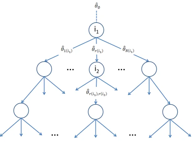
2. Representing an Unconstrained CAT in a Tree Structure 131

In this section we show that a CAT without exposure control can be repre-132

sented in a tree structure. This representation enables a fast selection (in the 133

order of milliseconds) of the items presented to the examinee. It also facilitates 134

the development of the models introduced in the following sections. The no-135

tation introduced herein will be used throughout the rest of the article and is 136

summarised in the Appendix. 137

Consider a test composed of I items that will be administered to J indi-138

viduals for assessing certain trait θ. For the sake of simplicity, and without 139

loss of generality, we assume that all items haveRpossible answers. When the 140

test is to be administered to participantj, the only information available is the 141

distribution of θin the population, given by the density function f(θ). Before 142

any item has been administered, it is frequent to assume that the value of this 143

trait for a particular examinee is given by the maximum off(θ). This value is 144

denoted by ˆθ∅.

145

The first item that is administered to this participant, ij1, is the one that 146

reaches the maximum value of a pre-established item selection criteria (FMI, 147

MEPV, KL, etc.) given ˆθ∅. We note that, when item exposure control is not

148

taken into account, the first item to be administered to all participants is the 149

same,ij₁, since ˆθ∅ is identical for all participants. Once the examinee responds

150

to this item, providing the answer r(ij₁) ∈ {1, ..., R}, his trait is re-assessed to 151

a new value ˆθ_uj

1, whereu j

1 =r(i

j

1) indicates the first item given to examinee j 152

and the answer provided. 153

This newly estimated value of the trait, ˆθ_uj

1, is then used to select the next

154

item to be presented to the examinee,ij₂. It is important noticing that all partic-155

ipants who provide the same answer to the first item will get the same estimate 156

ˆ θ_uj

1, and will therefore be given the same second item. Once the examinee has

157

answered to the new item, the estimated value of the trait is updated to ˆθ_uj

2

158

whereuj₂={r(i₁j), r(ij₂)}. 159

This way, subsequent items are administered iteratively until a given crite-160

rion is reached. Briefly, when examinee j has responded to the firstnitems by 161

obtaining the response pattern uj

n = {r(i j

1), . . . , r(ijn)}, a new estimate of the

162

trait, ˆθ_uj

n, is calculated and the next item is selected based on this value. All 163

those examinees who share the same response pattern uj

n to the first n items

164

will be given the same item n+ 1. Based on this discussion, a CAT can be 165

i

i

Figure 1: Tree Representation of a CAT.

3. Building a CAT with Minimum MSE 167

DTs are supervised methods built by minimising the square error in the es-168

timation of an explanatory variable (Rokach and Maimon, 2014). As mentioned 169

above, the available research work using the DT methodology as an alternative 170

for CATs, use either the total test’s score (Yan et al., 2004; Ueno and Song-171

muang, 2010) or an external criterion as dependent variable (Delgado-Gomez 172

et al., 2016; Riley et al., 2011). In this section we present a methodology for 173

building a DT that minimises the MSE in the trait’s estimation (instead of the 174

test score used in the aforementioned works). The MSE in the estimation of the 175

trait is the most frequently used criterion for building DTs and for assessing the 176

accuracy of a CAT. 177

In the design of this CAT, we start by building the root of the tree. Take 178

an item ifrom the test battery. Let θ be the actual trait of a person, j, who 179

answers this item;pi(r|θ), the probability that this person will give the answer

180

r∈ {1, ..., R}; and ˆθr, the value of the trait estimated for each of the possible

181

answers. The MSE of this item for this person is 182

Ei(θ|∅) = R X

k=1

(θ−θˆ_vjk

1)

2

pi(k|θ) (1)

where the empty set in the expectation emphasises the fact that no item has 183

yet been administered; andvk

1 ={r(i) =k}. The MSE that will be obtained if 184

itemiis administered to the population is, consequently, given by 185

Ei= Z

The starting item,i1, which constitutes the root of the tree, will be the one for 186

which the valueEi is minimal.

187

Once the tree root has been defined, theRitems corresponding to its children 188

will be added as follows: if itemi6=i1 is administered after an examinee with 189

real trait θ chose ther-th answer to item i1, the MSE of this person will be 190

given by 191

Ei(θ|u1) =

R X

k=1

(θ−θˆvk

2)

2_p

i(k|θ) (3)

wherev2k={u1, r(i) =k}and ˆθvk

2 is the estimated trait considering patternv k

2. 192

Therefore, the MSE of the group that gave answer rto itemi1 is given by 193

Ei= Z

Ei(θ|u1)f(θ|u1)dθ (4)

where 194

f(θ|u1) =

p(u1|θ)f(θ) p(u1)

= pR(r(i1)|θ)f(θ) p(r(i1)|θ)dθ

(5)

In general, given an individual with trait θ and response pattern un =

195

{r(i1), ..., r(in)}, the MSE obtained if unused item i is administered next can

196

be written as 197

Ei(θ|un) = R X

k=1

(θ−θˆvk n+1)

2_p

i(k|θ) (6)

where vk

n+1 ={un, r(i) = k}. Then, the MSE of a group of participants that

198

has followed patternun becomes

199

Ei= Z

Ei(θ|un)f(θ|un)dθ (7)

where 200

f(θ|un) =

p(un|θ)f(θ)

p(un)

=

Qn

j=1p(r(ij)|θ)f(θ)

R Qn

j=1p(r(ij)|θ)dθ

(8)

3.1. Computational Issues

201

An important aspect that needs to be addressed is how to efficiently build the 202

tree, as the number of nodes grows exponentially when the tree expands. Below 203

we discuss three strategies aimed, the first two, at speeding-up the construction; 204

and, the last one, at keeping the number of nodes within reasonable limits. 205

Parallel programming. Nodes within the same level are constructed inde-206

pendently. Therefore, the items that constitute these nodes can be determined 207

using parallel programming. For example, if a tree developed in a personal com-208

puter with four cores was programmed in parallel, the time required to build 209

it would be reduced to 25 percent of the time required time in a single core. 210

Currently, most universities and research centres have small clusters with a few 211

thousand cores available, making the development of the proposed methodology 212

easily attainable. 213

Passing information from parent to child nodes. As seen in formula 214

(8), to calculate the posterior probability of the ability level, it is necessary to 215

already been calculated in the parent node, if this information is stored, only 217

one multiplication is required for each child node and item pair. 218

Merging branches. One way for limiting the growth in the number of 219

nodes is joining together those branches that lead to similar estimates of ability 220

level. As an example, if an accuracy of 0.001 is set –which is a quite sensible 221

bound-, and assume that the ability takes values between -4 and 4, the maximum 222

number of nodes in each of the tree’s levels will be only 8000, which is a more 223

manageable number than the Rℓ nodes that may potentially appear at levelℓ. 224

An alternative method, frequently used in DT design, for controlling the size 225

of the tree is pruning some branches. In our case this will imply stopping the 226

growth of the tree in nodes associated to improbable answer patterns. However, 227

this may in practice give raise to situations where one of these nodes is actually 228

visited, implying that an on-line selection of the remaining items in the CAT will 229

need to be conducted. This would considerably increase the duration of the test 230

if the item selection criteria used is among the most computationally expensive 231

ones. For this reason we do not consider this practice a good alternative to 232

branch merging. 233

3.2. Equivalence of Minimum MSE and Minimum EPV

234

In this section we establish an interesting result: building a DT minimis-235

ing the MSE is mathematically equivalent to building a CAT where the item 236

selection criterion is the minimum EPV. 237

As discussed around equations (6) to (8), the MSE can be written as 238

M SE =

Z

p(θ|uj−1)

R X

r=1

pi(r|θ)(θ−θˆuj) 2

dθ (9)

which becomes 239

=

Z _XR

r=1

p(θ|uj−1)pi(r|θ)(θ−θˆuj)

2_{dθ (10)}

and using Bayes theorem 240

=

Z _XR

r=1

p(uj−1|θ)p(θ) p(uj−1)

pi(r|θ)(θ−θˆuj) 2

dθ (11)

using the local independence condition this equation can be simplified to 241

=

Z _XR

r=1

p(uj|θ)p(θ)

p(uj−1)

(θ−θˆuj)

2_{dθ (12)}

after multiplying and dividing bypi(r|uj−1) we get 242

=

Z _XR

r=1

p(uj|θ)p(θ)pi(r|uj−1) p(uj−1)pi(r|uj−1)

(θ−θˆuj) 2

dθ (13)

=

Z _XR

r=1

p(uj|θ)p(θ)pi(r|uj−1) p(uj)

(θ−θˆuj) 2

dθ (14)

using Bayes agaoin, this expression can be further simplified to 244

=

Z _XR

r=1

p(θ|uj)pi(r|uj−1)(θ−θˆuj)

2_{dθ (15)}

finally, after reordering terms we get 245

=

R X

r=1

pi(r|uj−1)

Z

p(θ|uj)(θ−θˆuj) 2

dθ=

R X

r=1

pi(r|uj−1)V ar(θ|uj) (16)

which is precisely the EPV criterion. 246

Consequently, notwithstanding the works discussed in the introduction treat 247

CATs and DTs as disjoint methods, in this section we have established the 248

equivalence between them. In practical terms, this implies that building a CAT 249

with minimal EPV is equivalent to constructing a DT minimising its standard 250

MSE criterion. This result suggests that when the objective of the CAT is 251

minimising the MSE, the most appropriate item selection criterion would be 252

EPV. 253

4. Tree-CAT: A CAT with Controlled Item Exposure Rate and Min-254

imum MSE 255

In this section, we propose a method for building a CAT that minimises 256

the MSE with controlled maximum exposure rate (proportion of the individuals 257

taking the test that receive a particular item) by building several decision trees 258

simultaneously. 259

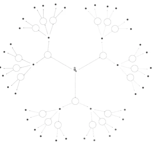
The underlying idea stems from the so-called randomesque method. At each 260

level, this method randomly selects the next item among the K items with the 261

best selection criteria values, given the current estimated ability ˆθ. For each 262

participant, randomesque starts selecting one of the K items attaining maximal 263

values for the selection criteria at the initial trait ˆθ0. Each of these items can 264

be seen as constituting the root of one of K trees. From each root will stem 265

R branches, corresponding to the R possible answers, each of them spanning 266

K nodes. This process is repeated at each level, ℓ, of the tree. Therefore, the 267

randomesque method can be visualised as a forest of K trees. This is represented 268

as a DTs forest in Figure 2 for R = 2 and K = 3. In this figure white items 269

Figure 2: Representation of randomesque method as a DTs forest.

Although this method reduces the item’s exposure, it does not prevent an 271

item from exceeding the maximum exposure rate. To address this problem, in 272

the following lines we present the Tree-CAT method. This method builds on 273

ramdomesque for generalising the method developed in the previous section. 274

Tree-CAT imposes a probabilistic bound to the maximum rate of item exposure 275

when creating the forest of trees. 276

Tree-CAT starts by selecting the K initial nodes. Let E be the vector 277

containing the items’ MSEs as computed by equation (2);D, a vector indicating 278

the items’ availability;P, a vector containing the probability of each item to be 279

administered as first item in the test; and rmax, the maximum item exposure

280

rate. Initially, each of the elements in D is set equal to the maximal exposure 281

rate. Given that 100% of the participants has to be assigned an item at the 282

beginning of the test, the algorithm utilises a capacity variable c to represent 283

the proportion of individuals that remain uncovered after each item is included. 284

Lis a very large number. The selection of the nodes and determination of their 285

number,K, is conducted as indicated in Algorithm 1. 286

The algorithm starts by selecting the itemiwith least MSE and associates 287

to this item the minimal value among its current availability,Di, and the

unas-288

signed capacity, c. This value, Pi, is then subtracted from both, the item’s

289

availability and the capacity variable. For guaranteeing that this item will not 290

be selected again, its value in vector E is replaced by a very large numberL. 291

This procedure is then repeated until c is equal to zero. The algorithm re-292

turns the set ofK=|F|initial nodes, and the administration probabilities and 293

updated availability vectors. 294

Once the K roots have been chosen, the trees spanned by each root will 295

grow jointly in an iteratively fashion. For the sake of clarity in the exposition, 296

Algorithm 1RootSpan Require: E, D

1: c:= 1

2: P:=0(I×1)

3: F:=∅

4: whilec >0 do

5: i:= argmin{E} 6: Pi:= min{c, Di}

7: c:=c−Pi

8: Di :=Di−Pi

9: F:=F ∪i

10: Ei:=L

11: end while Ensure: F, D, P

LetEbe a matrix whose elementEijis the MSE incurred if itemiwas added

to branch j, where each j is given by a different root/answer combination, i.e. j = R×(k−1) +r for k = 1, . . . , K;r = 1, . . . , R. Let C be a vector containing the proportion of participants associated with branch j, whereCj=

Pk R

P(r|θ, ik)f(θ)dθ and PjCj = 1. Let D be the available capacity vector

returned by Algorithm 1. Then, the choice of the items associated with each of the branches is done by means of the following linear program:

min X

i X

j

XijEij (17)

s.t. X

i

Xij ≤Di X

j

Xij =Cj

This simple model minimises the MSE subject to the constraints that not 298

item will exceed its availability; and that all participants must be given a sec-299

ond item during the test. Further levels of the trees are obtained by successive 300

applications of this procedure, with system (17) solved over the matrix E ob-301

tained for the corresponding item/response combination (henceforth referred to 302

as branch); the last update of vector D; and a newly obtained vectorC where 303

Cj=Pk R

P(r|θ, uk−1)f(θ)dθ. 304

Unfortunately, the number of constraints grows exponentially on the number 305

of levels, making the linear program computationally intractable. A computa-306

tionally efficient heuristic, illustrated in Algorithm 2, has been developed for 307

addressing this problem. 308

Algorithm 2 can be seen as a bi-dimensional extension of Algorithm 1. Work-309

ing with inherited vector D and matrices E and C as inputs, the Algorithm 310

returns an arrayF of sets of items for all possible branches stemming from the 311

previous level. It also returns a matrixP containing the relative probability for 312

each item to be administered to an individual in a given branch, and a vector 313

D with the updated items’ availability. 314

Algorithm 2Growing the tree Require: E, D,C

1: c:= 1

2: P:= (0)I×RK

3: F:={F1, . . . ,FRK},Fh:=∅ ∀h= 1, . . . , RK

4: whilec >0 do

5: forj≤I do

6: if Dj == 0then

7: Ej•:=L

8: end if

9: end for

10: (i, j) := argmin{E} 11: Pij:= min{Cj, Di}

12: Di :=Di−Pij

13: c:=c−Pij

14: Fj:=Fj∪i

15: Ei,j:=L

16: end while Ensure: F, D, P

assigned more than one item. The reason for this is that the best item for a 316

given node may not have the required capacity (i.e. Dj< Cj).

317

5. Numerical Experiments: Simulated Data 318

In this section we present the results of an experimental assessment of the 319

performance of the Tree-CAT method. The experiment compares our method 320

with three other available methods designed for controlling item exposure, namely, 321

restrictive (disallows the use of items that exceed the maximum rate), item eligi-322

bility (restricts the likelihood of administering an item to a given exposure rate), 323

and randomesque methods (randomly selects the next item from a subset of the 324

most informative items). In order to achieve a fair comparison between the 325

four methods, MEPV is used in all of them as the item selection criteria. This 326

choice is due to the fact that, as shown in Section 3.2, this criterion minimises 327

the MSE. 328

5.1. Data and experimental set-up

329

The experiment set-up is similar to the one used by other authors when 330

comparing item exposure control techniques in CATs (Pastor et al., 2002). In 331

detail, the item bank consists of 100 items with randomly generated parameters 332

according to Samejima’s graded response model (Samejima, 2016). Each item’s 333

discrimination parameter was generated following a log-normal distribution with 334

zero mean and standard deviation equal to 0.1225. The difficulty parameters 335

were generated following a standard normal distribution (Magis and Raˆıche, 336

2011). The maximum exposure rate was set to 0.3 with test length equal 10. 337

This length is considered to be enough for comparing the different methods 338

and it is similar to the one appearing in recent works. For example, CATs 339

(2016), for assessing different clinical conditions, used averages of 4, 5.3 and 6 341

items, respectively. Regarding the randomesque method, the number of random 342

alternatives available for each node at each level of the tree is set to six. 343

The performance of the CATs was evaluated by means of the answers of 344

500 randomly generated examinees (Magis et al., 2012). Given the random 345

nature of the item selection of three of the used procedures (randomesque, item 346

eligibility and ours), and to avoid path dependence in the results, the test was 347

repeated 25 times for each examinee and means were taken. In order to improve 348

the significance of the results, this scenario was repeated 10 times. 349

5.2. Results

350

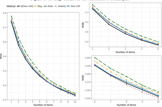
Figure 3 shows the evolution of MSE attained by each of the techniques 351

during the test execution. The large panel shows the entire execution, with 352

the two small panels being zoomed-in versions of the performance over the 353

first and last five items, respectively. The dot-dash yellow line represents the 354

eligibility method; the dash green line, the restrictive method; the dotted line, 355

the randomesque method; and the the solid blue line, the Tree-CAT method. 356

An extra line, solid black, shows the theoretical expected MSE corresponding 357

to the Tree-CAT method. 358

Figure 3: Average MSEs for the Alternative Techniques

0.2 0.3 0.4 0.5 0.6 0.7 0.8

1 2 3 4 5 6 7 8 9 10

Number of items

MSE

Method E[Tree−CAT] Eleg. Restr. RndmQ Tree−CAT

0.4 0.5 0.6 0.7

1 2 3 4 5

Number of items

MSE

0.225 0.250 0.275 0.300 0.325 0.350

6 7 8 9 10

Number of items

MSE

The figure shows that the Tree-CAT method obtains more precise estimates 359

than the eligibility and the restricted methods in terms of MSE. This graph 360

also shows that the Tree-CAT attains a performance close to the theoretically 361

expected one. Finally, the randomesque method shows a slightly better perfor-362

mance than the Tree-CAT from the seventh item administered on. This can 363

be explained by looking at the overlap rate, which is a common measure of 364

test security defined as the percentage of common items for any two randomly 365

overlap rates are 0.268 for restrictive; 0.275 for eligibility; 0.283 for Tree-Cat; 367

whereas it reaches 0.538 for randomesque. 368

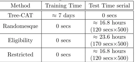
Regarding the computation time, Table 1 shows the time needed to create 369

the DT as well as the minimum time required by each of the methods to se-370

lect the 10 items for the 500 participants. It is important to note here that 371

in both, item eligibility and restricted methods, participants receive the test 372

sequentially. That is, in order to recalculate the parameters, the current par-373

ticipant must have finished the test before the next one receives it. In contrast, 374

randomesque and Tree-CAT methods are able to administer the test simulta-375

neously. Moreover, whereas the tree alternative methods select the next item 376

on-line, Tree-CAT generates the whole tree at once, which means that the time 377

required for generating the next item is, indeed, zero. The experiment was con-378

ducted using 128 cores of a cluster with a Xeon 2630 processor and 32 GB of 379

RAM. 380

Table 1: Training and Execution Times

Method Training Time Test Time serial

Tree-CAT ≈7 days 0 secs

Randomesque 0 secs ≈16.8 hours

(120 secs×500)

Eligibility 0 secs ≈23.6 hours

(170 secs×500)

Restricted 0 secs ≈16.8 hours

(120 secs×500)

According to the table, the randomesque, restricted and eligibility methods 381

take 2 minutes for selecting the items. In practical terms this means that the ex-382

aminee will need to wait 12 seconds in average before the next item is provided. 383

These long execution times are explained, firstly, by the use of MEPV, which 384

has a high computational cost. More economical item selection methods such 385

as FMI could render better results in terms of computational times, at the cost 386

of incurring the problems highlighted in the introduction to this paper. Sec-387

ondly, those long times can also be attributed to the use of the implementation 388

catR (Magis and Raˆıche, 2011), which does not use any of the two speeding-up 389

strategies described in Section 3.1. It should be said that, even if those strate-390

gies were implemented, the eligibility and restrictive method still suffer from the 391

sequential application burden, which imposes a serious penalty in the execution 392

time (23.6 and 16.8 hours for 500 administrations of the test). 393

It is also important to mention that the cost in computational time incurred 394

by the three alternative methods discussed in this section is paid every time the 395

test is conducted. With the Tree-CAT method, in contrast, once the trees are 396

built and all the alternative sequences stored, the time between the answer and 397

the selection of the next item is –to all practical extent- zero, regardless the 398

number of participants. This feature enables the simultaneous on-line applica-399

tion of the test to an unlimited number of participants, something that is not 400

possible with the other methods. Hypothetically, this could be attained with 401

randomesque, but in this case the simultaneous application of the test to a large 402

number of people will require the availability of a server with as many nodes as 403

6. Numerical Experiments: Real Data 405

This section evaluates the proposed methodology using actual data. These 406

data have been obtained from a previous study (Rubio et al., 2007), in which a 407

psychometric scale for measuring emotional adjustment was developed. Before 408

presenting the experimental results, in the following section we describe both 409

the data set and the design of the experiment. 410

6.1. Data and experimental set-up

411

The data in this study contain the answers provided by 792 psychology stu-412

dents to the 28 items of the Emotional Adjustment Bank (Rubio et al., 2007). 413

For our experiments, it was considered that the item responses have three levels 414

(”disagree”, ”neutral” and ”agree”). For testing the unidimensionality of the 415

scale, a factor analysis in conjunction with a parallel analysis (Hayton et al., 416

2004) showed that only one factor is retained. This confirms the unidimension-417

ality and justifies the use of a graded response model. 418

In order to compare the performance of the Tree-CAT method against the 419

chosen exposure control methods (Restrictive, Eligibility, Randomesque) under 420

conditions similar to the real ones, the hold-out validation method was used. 421

Specifically, the data set was randomly divided into two disjoint subsets of equal 422

size: the training set and the test set. The training set was used to estimate 423

the different items’ parameters and to build the DT for the Tree-CAT method, 424

whereas, the test set was used for the comparisons. It was assumed that the 425

traitsθ of the participants were those obtained when the 28 items of the bank 426

were administered to them. The test length was set to 7 items. The remaining 427

parameters that define the experiment have been set to the same values as 428

those of the simulation study in Section 5. Namely, the MEPV was chosen 429

as item selection criterion; the maximum exposure rate was fixed at 0.3; and 430

the number of random alternatives for the Randomesque method was set to 431

6. As before, in order to avoid path dependence, the test was repeated 25 432

times for each examinee, and means were taken for the Tree-CAT, Elegibility 433

and Randomesque methods. In addition, to achieve more reliable results, this 434

scenario was simulated 10 times. 435

6.2. Results

436

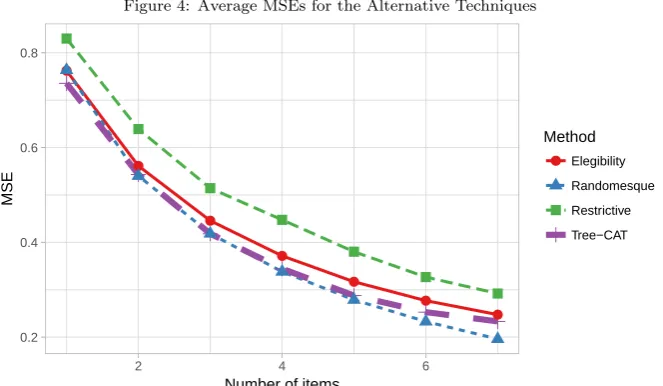
Figure 4 shows the MSE obtained by the different techniques as a func-437

tion of the number of items administered to the subjects. It can be noticed 438

that, except for the Randomesque method in the last levels, Tree-CAT is the 439

one achieving the best performance (based on the MSE). As explained in the 440

discussion to our simulated experiments, the reason why Randomesque outper-441

forms the other three methods at the last levels of the test is that it exceeds the 442

maximum exposure rate. The overlap rates of Tree-CAT, Restrictive, Eligibility 443

and Randomesque methods are 0.28, 0.28, 0.29 and 0.58, respectively. 444

Table 2 depicts the computational time used to construct the decision tree 445

for the Tree-CAT method, and the time needed to select the next item for each 446

of the four techniques. These numbers are similar to those obtained in Table 447

1 of the previous experiment on a smaller scale, as the item bank used in this 448

study is 28% the size of the previous one, and the length of the test is 7 items 449

Figure 4: Average MSEs for the Alternative Techniques

0.2 0.4 0.6 0.8

2 4 6

Number of items

MSE

Method

Elegibility

Randomesque

Restrictive

Tree−CAT

Table 2: Training and Execution Times

Method Training Time Test Time serial

Tree-CAT ≈36 min. 0 secs

Randomesque 0 secs ≈103 min.

(15.6 secs×396)

Eligibility 0 secs ≈117 min.

(17.7 secs×396)

Restricted 0 secs ≈103 min.

(15.6 secs×396)

7. Conclusion 451

In this article, we present a new method for building CATs, referred to as 452

Tree-CAT, based on the DTs methodology. The proposed method creates and 453

stores a representation of the CAT in a tree structure that allows items to be 454

selected in milliseconds. This property is especially valuable when the chosen 455

item selection method involves the calculation of integrals (e.g. when a CAT 456

uses minimal EPV for item selection). In this regard, it is demonstrated that 457

building a CAT that minimises the EPV is equivalent to building a DT that 458

minimises the MSE. 459

In the article we also show that creating a CAT with item exposure controls 460

can be understood as the simultaneous construction of several trees, and propose 461

an algorithm for performing this task. This algorithm allows the use of different 462

strategies that accelerate its construction. First, it is possible to use parallel 463

programming to calculate the MSE matrix required by the algorithm. Second, 464

the calculation of MSEs can be simplified using information obtained at the 465

previous level nodes. Finally, it seems possible to merge branches that produce 466

similar estimates of the trait level, allowing the tree to be kept within reasonable 467

dimensions. In this article we have conducted experiments taking advantage of 468

Tree-CAT presents several advantages with respect to other existing meth-470

ods. Firstly, the results obtained experimentally show that Tree-CAT is the 471

method with the lowest MSE among those with the lowest overlap rate. An-472

other advantage is that it can potentially be administered simultaneously to an 473

unlimited number of participants. In contrast to existing methods, which calcu-474

late in real time each of the items to be presented based on previous answers, the 475

Tree-CAT selects the next item to be presented from a previously stored struc-476

ture. This allows, for practical purposes, to eliminate the time required for item 477

selection. This is especially useful when item selection criteria are computa-478

tionally expensive. These two properties, namely, simultaneous application and 479

zero time in the selection of items, make Tree-CAT an ideal candidate for the 480

simultaneous administration of on-line tests to a large number of participants. 481

One weakness of the method is the need of a small computer cluster for build-482

ing the tree within reasonable time. For example, in the experiment developed 483

in this article, 128 nodes of a cluster were used. However, the availability of a 484

larger cluster could reduce the construction time of the tree from one week –as 485

in our case- to a few hours. The importance of this limitation is further reduced 486

by the fact that, once the tree has been built, the test can be administered from 487

any personal computer. 488

Regarding this limitation, an appealing future research line consists of find-489

ing a mechanism for optimally merging the branches of the trees in order to limit 490

the size of the trees. Additional research could also be developed for address-491

ing issues like content balance, variable test length, or multidimensional-trait 492

assessment. 493

We conclude the article by stating our conviction, supported by the exper-494

imental and analytical results obtained, that the DTs approach for building 495

CATs is a promising research line that opens up several lines of research and 496

combines the knowledge of the areas of Psychology, Statistics, Operational Re-497

search and Computer Science. 498

Acknowledgments 499

Numerical experiments were conducted in Uranus, a supercomputer cluster 500

located at Universidad Carlos III de Madrid and jointly funded by EU-FEDER 501

funds and by the Spanish Government via the National Projects No. UNC313-502

4E-2361, No. ENE2009-12213- C03-03, No. 33219, No. ENE2012-503

31753 and No. ENE2015-68265-P. 504

References 505

Armstrong, R. and Edmonds, J. (2004). A study of multiple stage adaptive test 506

designs. In annual meeting of National Council of Measurement in

Educa-507

tion,(NCME), San Diego, CA. 508

Barrada, J. R., Olea, J., and Ponsoda, V. (2007). Methods for restricting 509

maximum exposure rate in computerized adaptative testing. Methodology:

510

European Journal of Research Methods for the Behavioral and Social Sciences, 511

Blasco-Fontecilla, H., Delgado-Gomez, D., Ruiz-Hernandez, D., Aguado, D., 513

Baca-Garcia, E., and Lopez-Castroman, J. (2012). Combining scales to 514

assess suicide risk. Journal of psychiatric research, 46(10):1272–1277. 515

doi:10.1016/j.jpsychires.2012.06.013. 516

Chang, H.-H. and Ying, Z. (1996). A global information approach to comput-517

erized adaptive testing. Applied Psychological Measurement, 20(3):213–229. 518

doi:10.1177/014662169602000303. 519

Chapman, D. S. and Webster, J. (2003). The use of technologies in the re-520

cruiting, screening, and selection processes for job candidates. International

521

journal of selection and assessment, 11(2-3):113–120. 522

De Beurs, D. P., de Vries, A. L., de Groot, M. H., de Keijser, J., and Kerkhof, 523

A. J. (2014). Applying computer adaptive testing to optimize online assess-524

ment of suicidal behavior: a simulation study. Journal of medical Internet

525

research, 16(9). doi:10.2196/jmir.3511. 526

Delgado-Gomez, D., Baca-Garcia, E., Aguado, D., Courtet, P., and Lopez-527

Castroman, J. (2016). Computerized adaptive test vs. decision trees: devel-528

opment of a support decision system to identify suicidal behavior. Journal of

529

affective disorders, 206:204–209. doi:10.1016/j.jad.2016.07.032. 530

Fliege, H., Becker, J., Walter, O. B., Bjorner, J. B., Klapp, B. F., and Rose, 531

M. (2005). Development of a computer-adaptive test for depression (d-cat). 532

Quality of life Research, 14(10):2277. 533

Gardner, W., Shear, K., Kelleher, K. J., Pajer, K. A., Mammen, O., Buysse, D., 534

and Frank, E. (2004). Computerized adaptive measurement of depression: a 535

simulation study. BMC psychiatry, 4(1):13. doi:10.1186/1471-244X-4-13. 536

Georgiadou, E. G., Triantafillou, E., and Economides, A. A. (2007). A review of 537

item exposure control strategies for computerized adaptive testing developed 538

from 1983 to 2005. The Journal of Technology, Learning and Assessment, 539

5(8). 540

Gibbons, R. D., Weiss, D. J., Frank, E., and Kupfer, D. (2016). Computerized 541

adaptive diagnosis and testing of mental health disorders. Annual review of

542

clinical psychology, 12. doi:10.1146/annurev-clinpsy-021815-093634. 543

Hayton, J. C., Allen, D. G., and Scarpello, V. (2004). Factor retention decisions 544

in exploratory factor analysis: A tutorial on parallel analysis. Organizational

545

research methods, 7(2):191–205. 546

Hsueh, I.-P., Chen, J.-H., Wang, C.-H., Chen, C.-T., Sheu, C.-F., Wang, W.-547

C., Hou, W.-H., and Hsieh, C.-L. (2016). Development of a computerized 548

adaptive test for assessing balance function in patients with stroke. Physical

549

therapy, 90(9):1336–1344. doi:10.2522/ptj.20090395. 550

Kingsbury, G. G. and Zara, A. R. (1989). Procedures for selecting items for 551

computerized adaptive tests. Applied measurement in education, 2(4):359– 552

Leung, Y. W., Brown, C., Cosio, A. P., Dobriyal, A., Malik, N., Pat, V., Irwin, 554

M., Tomasini, P., Liu, G., and Howell, D. (2016). Feasibility and diagnostic 555

accuracy of the patient-reported outcomes measurement information system 556

(PROMIS) item banks for routine surveillance of sleep and fatigue problems in 557

ambulatory cancer care. Cancer, 122(18):2906–2917. doi:10.1002/cncr.30134. 558

Lord, F. M. (1980). Applications of item response theory to practical testing

559

problems. Hillsdale, NJ: Lawrence Erlbaum. 560

Lu, P., Zhou, D., Qin, S., Cong, X., and Zhong, S. (2012). The study of 561

item selection method in cat. In Computational Intelligence and Intelligent

562

Systems, pages 403–415. Springer. doi:10.1007/978-3-642-34289-9 45. 563

Magis, D. and Raˆıche, G. (2011). catR: An R package for computer-564

ized adaptive testing. Applied Psychological Measurement, 35(7):576–577. 565

doi:10.1177/0146621611407482. 566

Magis, D., Raˆıche, G., et al. (2012). Random generation of response patterns 567

under computerized adaptive testing with the r package catR. Journal of

568

Statistical Software, 48(8):1–31. doi:10.18637/jss.v048.i08. 569

Moore, T. M., Calkins, M. E., Reise, S. P., Gur, R. C., and Gur, R. E. 570

(2018). Development and public release of a computerized adaptive (CAT) 571

version of the schizotypal personality questionnaire. Psychiatry research. 572

doi:10.1016/j.psychres.2018.02.022. 573

Pastor, D. A., Dodd, B. G., and Chang, H.-H. (2002). A comparison of item se-574

lection techniques and exposure control mechanisms in cats using the general-575

ized partial credit model.Applied Psychological Measurement, 26(2):147–163. 576

doi:10.1177/01421602026002003. 577

Revuelta, J. and Ponsoda, V. (1998). A comparison of item exposure control 578

methods in computerized adaptive testing. Journal of Educational

Measure-579

ment, 35(4):311–327. doi:10.1111/j.1745-3984.1998.tb00541.x. 580

Riley, B., Funk, R., Dennis, M.and Lennox, R., and Finkelman, M. (2011). The 581

use of decision trees for adaptive item selection and score estimation. In

An-582

nual Conference of the International Association for Computerized Adaptive

583

Testing. 584

Rokach, L. and Maimon, O. (2014). Data mining with decision trees: theory

585

and applications. World scientific. 586

Rubio, V. J., Aguado, D., Hontangas, P. M., and Hern´andez, J. M. (2007). 587

Psychometric properties of an emotional adjustment measure: An application 588

of the graded response model.European Journal of Psychological Assessment, 589

23(1):39–46. 590

Samejima, F. (2016). Graded response models. In Handbook of Item Response

591

Theory, Volume One, pages 123–136. Chapman and Hall/CRC. 592

Shin, C. D. (2017). Conditional randomesque method for item exposure control 593

in cat. International Journal of Intelligent Technologies & Applied Statistics, 594

Stucky, B. D., Edelen, M. O., Sherbourne, C. D., Eberhart, N. K., and Lara, 596

M. (2014). Developing an item bank and short forms that assess the im-597

pact of asthma on quality of life. Respiratory medicine, 108(2):252–263. 598

doi:10.1016/j.rmed.2013.12.008. 599

Sympson, J. and Hetter, R. (1985). Controlling item-exposure rates in com-600

puterized adaptive testing. In Proceedings of the 27th annual meeting of the

601

Military Testing Association, pages 973–977. 602

Tseng, W.-T. (2016). Measuring english vocabulary size via computerized adap-603

tive testing. Computers & Education, 97:69–85. 604

Ueno, M. and Songmuang, P. (2010). Computerized adaptive testing 605

based on decision tree. In Advanced Learning Technologies (ICALT),

606

2010 IEEE 10th International Conference on, pages 191–193. IEEE. 607

doi:10.1109/ICALT.2010.58. 608

van der Linden, W. J. (2003). Some alternatives to sympson-hetter item-609

exposure control in computerized adaptive testing. Journal of Educational

610

and Behavioral Statistics, 28(3):249–265. doi:10.3102/10769986028003249. 611

van der Linden, W. J. and Glas, C. A. (2000). Computerized adaptive testing:

612

Theory and practice. Springer. 613

van der Linden, W. J. and Pashley, P. J. (2009). Item selection and ability 614

estimation in adaptive testing. InElements of adaptive testing, pages 3–30. 615

Springer. doi:10.1007/978-0-387-85461-8 1. 616

van der Linden, W. J. and Veldkamp, B. P. (2005). Constraining item exposure

617

in computerized adaptive testing with shadow tests, volume 2. Law School 618

Admission Council. 619

van der Linden, W. J. and Veldkamp, B. P. (2007). Conditional item-620

exposure control in adaptive testing using item-ineligibility probabili-621

ties. Journal of Educational and Behavioral Statistics, 32(4):398–418. 622

doi:10.3102/1076998606298044. 623

Veerkamp, W. J. and Berger, M. P. (1997). Some new item selection criteria for 624

adaptive testing.Journal of Educational and Behavioral Statistics, 22(2):203– 625

226. doi:10.3102/10769986022002203. 626

Veldkamp, B. P. and Matteucci, M. (2013). Bayesian computerized adaptive 627

testing. Ensaio: Avalia¸c˜ao e Pol´ıticas P´ublicas em Educa¸c˜ao, 21(78):57–82. 628

doi:10.1590/S0104-40362013005000001. 629

Weiss, D. J. (1982). Improving measurement quality and efficiency 630

with adaptive testing. Applied psychological measurement, 6(4):473–492. 631

doi:10.1177/014662168200600408. 632

Weiss, D. J. (2004). Computerized adaptive testing for effective and efficient 633

measurement in counseling and education. Measurement and Evaluation in

634

Weissman, A. (2007). Mutual information item selection in adaptive classi-636

fication testing. Educational and Psychological Measurement, 67(1):41–58. 637

doi:10.1177/0013164406288164. 638

Yan, D., Lewis, C., and Stocking, M. (2004). Adaptive testing with regres-639

sion trees in the presence of multidimensionality. Journal of Educational and

640

Appendix A. Notation 642

Section 2 643

J: set of participants; 644

I: item bank; 645

ij

n: n–th itemi∈ I to be administered to participantj∈ J;

646

R: number of possible answers to an item; 647

r(ij

n): answer of individualj∈ J to item ijn, i= 1, . . . , R.

648

θ: real-valued random variable describing a trait; 649

f :R→R+ density function ofθ; 650

ˆ

θ∅: argmaxθ∈_Rf(θ);

651

ujn: sequence of items and responses of individualj, withujn ={r(i j

k)}k=0,...,n

652

anduj0=∅; 653

ˆ θ_uj

n: estimatedθgiven patternu

j n;

654

Section 3 655

pi(un): probability of observing sequence un in a participant;

656

pi(r|θ): probability that a participant with traitθ will answerr∈ {1. . . R}to

657

itemi∈ I; 658

p(un|θ): probability that a participant with traitθwill show response sequence

659

un up to then-th item shown;

660

p(θ|un): posterior probability of traitθ given a response sequenceun;

661

vnk: sequence of items and responses if an individual with sequenceun−1chooses 662

answerk∈ {1,2. . . R}to then–th item. 663

ˆ θ_vj

n: estimatedθgiven patternv

j n.

664

Section 4 665

Xij: capacity of itemiassigned to branchj;

666

Eij: MSE incurred if itemi is added to branchj;

667

Di: capacity availability vector for itemi;

668

Cj: proportion of participants associated to branchj.