A classification scheme for turbulence based on the velocity-intermittency structure with an application to near-wall flow and with implications for bedload transport

velocity-intermittency structure with an application to near-wall flow and with implications

for bedload transport

.

White Rose Research Online URL for this paper:

http://eprints.whiterose.ac.uk/78411/

Version: Published Version

Article:

Keylock, CJ, Nishimura, K and Peinke, J (2012) A classification scheme for turbulence

based on the velocity-intermittency structure with an application to near-wall flow and with

implications for bedload transport. Journal of Geophysical Research, 117 (F1).

https://doi.org/10.1029/2011JF002127

[email protected] https://eprints.whiterose.ac.uk/

Reuse

Unless indicated otherwise, fulltext items are protected by copyright with all rights reserved. The copyright exception in section 29 of the Copyright, Designs and Patents Act 1988 allows the making of a single copy solely for the purpose of non-commercial research or private study within the limits of fair dealing. The publisher or other rights-holder may allow further reproduction and re-use of this version - refer to the White Rose Research Online record for this item. Where records identify the publisher as the copyright holder, users can verify any specific terms of use on the publisher’s website.

Takedown

If you consider content in White Rose Research Online to be in breach of UK law, please notify us by

A classification scheme for turbulence based on the

velocity-intermittency structure with an application to near-wall

flow and with implications for bed load transport

C. J. Keylock,

K. Nishimura,

and J. Peinke

Received 15 June 2011; revised 30 November 2011; accepted 6 February 2012; published 29 March 2012.

[1]

Kolmogorov

’

s classic theory for turbulence assumed an independence between

velocity increments and the value for the velocity itself. However, recent work has called

this assumption in to question, which has implications for the structure of atmospheric,

oceanic and fluvial flows. Here we propose a conceptually simple analytical framework

for studying velocity-intermittency coupling that is similar in essence to the popular

quadrant analysis method for studying near-wall flows. However, we study the dominant

(longitudinal) velocity component along with a measure of the roughness of the signal,

given mathematically by its series of Hölder exponents. Thus, we permit a possible

dependence between velocity and intermittency. We compare boundary layer data

obtained in a wind tunnel to turbulent jets and wake flows. These flow classes all have

distinct characteristics, which cause them to be readily distinguished using our technique

and the results are robust to changes in flow Reynolds numbers. Classification of

environmental flows is then possible based on their similarities to the idealized flow

classes and we demonstrate this using laboratory data for flow in a parallel-channel

confluence. Our results have clear implications for sediment transport in a range

of geophysical applications as they suggest that the recently proposed impulse-based

methods for studying bed load transport are particularly relevant in domains such

as gravel bed river flows where the boundary layer is disrupted and wake interactions

predominate.

Citation: Keylock, C. J., K. Nishimura, and J. Peinke (2012), A classification scheme for turbulence based on the velocity-intermittency structure with an application to near-wall flow and with implications for bed load transport,J. Geophys. Res.,117, F01037, doi:10.1029/2011JF002127.

1.

Introduction

[2] One assumption that underpins Kolmogorov’s classic analysis of scaling properties in turbulence [Kolmogorov, 1941] is that the values for the velocity increments are independent of the values for the velocity, which explains why many analyses derive results for the statistics of the velocity increments independent of the velocity itself [She and Leveque, 1994]. However, experimental [Praskovsky et al., 1993; Sreenivasan and Stolovitzky, 1996] and theo-retical [Hosokawa, 2007] work has called this assumption in to question and a recent attempt to model the velocity increments in the flow stochastically has found improved results with the inclusion of a velocity-dependent drift term

in the relevant Fokker-Planck equation for the velocity increments [Stresing and Peinke, 2010].

[3] This paper is motivated by such work and given the complex nature of geophysical flows it would seem impor-tant to examine if any similar dependency exists as these may be of some significance for developing improved tur-bulence closure schemes for problems involving pollutant dispersal or sediment entrainment. However, rather than adopting complex stochastic analysis methods to study such phenomena we were also motivated by the need to develop a simple tool for determining a dependency between velocity and the velocity increments, or variables directly related to scaling properties of the increments. This forms the primary contribution of this paper and we show that the graphical technique we develop can be used as a means for comparing different turbulent flows, and for classifying environmental flows relative to benchmark fluid mechanics cases. Impli-cations of our results for sediment transport are then dis-cussed toward the end of the manuscript. However, before we embark on describing our method, we first briefly review relevant parts of turbulence theory and describe formal analysis methods for characterizing the dependency between velocity and velocity increments.

1

Department of Civil and Structural Engineering, University of Sheffield, Sheffield, UK.

2

Graduate School of Environmental Studies, Nagoya University, Nagoya, Japan.

3

Institute of Physics and ForWind, University of Oldenburg, Oldenburg, Germany.

Copyright 2012 by the American Geophysical Union. 0148-0227/12/2011JF002127

JOURNAL OF GEOPHYSICAL RESEARCH, VOL. 117, F01037,doi:10.1029/2011JF002127, 2012

1.1. The Moments of Velocity Increments and Their Analysis

[4] If one studies the longitudinal velocity increments for a turbulent flow,vr=ux+r ux, as a function of the

sepa-ration, r, Kolmogorov-style scaling implies that the scaling law for the moments,n, ofvris self-similar:

hjvrj in∝jrxn

ð1Þ

where the Kolmogorov [1941] proposal is that xn = 1₃n.

However, because the energy dissipation for turbulent flows is intermittent, this model has been refined in various ways over the years to yield multifractal scalings [Kolmogorov, 1962; She and Leveque, 1994]. An alternative approach to an analysis of moments is to study all the moments at once via a direct study of the probability distribution function for

vras a function ofr.A method for doing this was introduced

by Friedrich and Peinke[1997] and applied to jet data by

Renner et al.[2001]. It considers turbulence to be a Markov process (as shown byHosokawa[2002]) and is based on an analysis of the conditional probability ofvr=l1as a function

of vr= l2,p(vr=l1|vr=l2), wherelis a length scale in the

flow,l1<l2…<lN,ljlies withinlj+ 1and the separation

between ljand lj + 1is more than a scale slightly smaller

than the Taylor scale termed the Einstein-Markov coherence length [Stresing and Peinke, 2010]. With the simplification to notation given by vlj ≡ vr=lj, one can study p(vl1| vl ∈ {2,3,N}), and if p(vl1|vl2) = p(vl1|vl ∈ {2,3,N}) then the

Markovian property holds and the problem may be greatly simplified, permitting a Fokker-Planck equation to be written for p(vl1|vl2) given some constraints on the fourth

order conditional moment for vl:

r∂

∂rpðvljjvlkÞ ¼ ½

∂ ∂vlj

D1ðvlj;rjÞ þ

∂2

∂v2 lj

D2ðvlj;rjÞ

pðvljjvlkÞ

ð2Þ

where k > j, and D1 and D2 are the drift and diffusion

coefficients. Renner et al. [2001] found thatD1was linear

in vl, while D2 was quadratic and that (2) could then be

used to derive the distribution functions p(vl) with high

accuracy. The generalization to include a possible velocity dependence for the increments was treated byStresing and Peinke [2010] where, if the Markovian property holds p

(vl1|vl2, ux) = p(vl1|vl ∈ {2,3,N}, ux) and the relevance of

conditioning on the velocity was determined by checking if p(vl1|vl2) =p(vl1|vl2,ux). This analysis found that while

there was no clear velocity dependence on the diffusion coefficient, there was for the drift coefficient and that the nature of this dependence depended on the type of flow studied. Hence, the assumption in Kolmogorov’_s

deriva-tion is not necessarily valid and the nature of the coupling between the flow and its increments depends on the type of flow considered as shown recently by Stresing et al.

[2010].

1.2. Relevance to Environmental Turbulence

[5] Given the complexity of environmental flows it seems probable that similar dependencies exist and these are important for understanding flow structures and, thus, ana-lyzing a suite of phenomena such as pollutant dispersal or

sediment entrainment. For example, if strong fluctuations in the data occur preferentially when the velocity is close to its mean, peak turbulent shear stresses will be lower than if strong fluctuations are coupled to higher mean velocities. Thus, this is not simply a question of fluid mechanics interest and it is important to test the extent to which fluid mechanics theory applies in the environment [Lovejoy et al., 2007]. However, the methods used to fit the Fokker-Planck equations in the studies by Peinke and co-workers are quite complex and require very long data sets, which may not be realistically obtainable for many geophysical flows. Hence, an alternative means for exploring this problem is needed. In the subsequent sections of this paper, we present such a method, apply it to high quality fluid mechanics data sets and then classify different types of flows. We use this flow classification to study the flow near the bed in the post confluence region in a laboratory channel and, finally, dis-cuss the implications of our results for sediment entrainment by fluvial processes.

2.

Analyzing the Coupling Between Velocity

and Velocity Increment Characteristics

[6] Quadrant analysis has a long history of use in studies of near-wall flow [Lu and Willmarth, 1973] and has been shown to be the most effective of traditional velocity-based methods for detecting near-wall sweeps and ejections [Bogard and Tiederman, 1986], which are of crucial importance for our understanding of near-wall flow [Adrian et al., 2000]. There has been considerable use of this method in environmental fluid mechanics, particularly in sedimen-tology where such processes are important for sediment transport and bed defect initiation [Best, 1992]. In general, it has been shown that of the two types of motion that con-tribute positively to the Reynolds stress near the wall, ejec-tions are more important for suspension transport [Niño and Garcia, 1996], while sweeps are more important for bed-load motion [Heathershaw and Thorne, 1985;Nelson et al., 1995]. However, the rarer outward ejections [Nakagawa and Nezu, 1977] are also important for bed load entrainment [Heathershaw and Thorne, 1985;Nelson et al., 1995]. Tra-ditional quadrants are based on a Reynolds decomposition of the instantaneous velocity measurements in the wall-parallel,

ux, and wall-perpendicular,uzdirections, e.g.u=x¼ux ux, where the / indicates a fluctuating quantity and the overbar a time-averaged mean. Four basic flow events can then be defined from this decomposition as given in Table 1. It is of course possible to take this further and identify flow struc-tures based on a decomposition of all three components and a classification into octants [Keylock, 2007].

[7] For the detection of particular near-wall structures, a threshold or hole size,H, is typically introduced to eliminate the incorrect classification of transient cases as true flow structures. For example, for the detection of ejectionsLuchik and Tiederman[1987] used a value forHof 1.21 to detect ejections. That is:

u=_xu=_{z Quad}2≥H½sðuxÞsðuzފ

ð3Þ

[8] Our method is based on quadrant analysis but rather than considering two velocity components or the vertical velocity component with an associated scalar [Katul et al., 1997], we consider a component of the velocity together with its associated series of pointwise Hölder exponents [Keylock, 2010]. In the appendix to this manuscript we outline the relation between velocity increments and Hölder exponents, which shows that our form of analysis may be related to the direct consideration of velocity and the scaling of velocity increments. Data are obtained as time series and converted into spatial series using a modified Taylor hypothesis [Kahalerras et al., 2007]. The series of pointwise Hölder exponents,ap(x,ux), is used to characterize the local

roughness of the velocity data where constant Hölder regu-larity implies a signal with a single Hurst exponent, or fractal dimension, while a signal with multifractal characteristics (such as turbulence) will haveap(x,ux) that varies spatially

depending on the presence of active flow structures. Periods of relative roughness are given by a lowap, withapdefined

over the interval 0 to 1 and apat a constant value of 0.5

corresponding to the Hurst exponent of a Brownian motion. Thus, this analysis is related to the calculation of the multi-fractal spectrum (MFS) of the velocity series [Meneveau and Sreenivasan, 1991; Muzy et al., 1991] but while the MFS gives, informally, the histogram of Hölder exponents,

ap(x,ux) estimates the Hölder exponent for each datum in a

discrete time series.

[9] For the remainder of this manuscript, we only consider the longitudinal velocity component,ux, and, consequently,

drop the subscript so thatu≡uxin much of our description.

An analysis of the series of Hölder exponents for multiple velocity components has been used recently to define active and inactive periods within environmental flows [Keylock, 2008], whereap(t,u) [orap(x,u)] can be obtained using a

fluctuation scaling theorem [Kolwankar and Lévy Véhel, 2002]. Thus, we consider the differentiability of a signal (its smoothness) relative to polynomial approximations about a particular point that is given by a Taylor series expansion:

pXðxÞ ¼ ∑ m 1

i¼0

ui_ðXÞ i! ðx XÞ

i _ð4Þ

where we study a velocity series,u(x), in a neighborhood,d, about a position, X, andmis the number of times thatuis differentiable in Xd.We then state thatu(x) has a point-wise Hölder exponent,ap(ux)≥0 if a constantK> 0 and the

polynomialpX(x) of degreemexist such that

uðxÞ pXðxÞ

j j≤Kjx Xb ð5Þ

The Hölder regularity,ap(ux), ofu(x) atXis then given by

the supremum (least upper bound) of b that fulfils equation (5).

[10] Accurate estimation of Hölder exponents can be undertaken in appropriate function spaces [Seuret and Lévy Véhel, 2003] or via refinements to the work of Jaffard

[1997] on wavelet bases. However, a simple and rapid method [Kolwankar and Lévy Véhel, 2002] is based on a log-log regression of the signal oscillations,OXd, within a

distance d of the location of interest, X, against d, where

OXdis given by:

OXd¼maxðux∈½X d;…;XþdŠÞ minðux∈½X d;…;XþdŠÞ ð6Þ

anddis distributed logarithmically. We adopt that approach here with logarithmically distributed bins ranging in size up to 213 data points (wind tunnel experiments) or 214 points (jet and wake data) for the analysis in section 4, but reduced to29 points for the shorter duration confluence-flow data in section 5. Convergence properties of this method as a function of the selected bin size were recently studied empirically byKeylock[2010] and performance was deemed better than wavelet-based methods.

[11] By subtracting their mean values to obtain fluctuating series, indicated by a prime, we can study the joint properties ofu/(x) andap

/

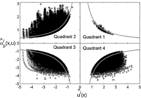
(x,u) and produce a four-way classification of the flow analogous to the conventional quadrant analysis explained in Table 1: {Q1:u/(x) > 0,ap/(x,u) > 0; fast and

smooth}, {Q2:u/(x) ≤0, ap/(x,u) > 0; slow and smooth},

{Q3: u/(x) ≤ 0, ap/(x, u) ≤ 0; slow and rough}, {Q4: u/(x) > 0,ap/(x,u)≤0; fast and rough}. An example analysis

is given in Figure 1 for a time series of 12.5 106 mea-surements on a turbulent jet obtained at 8 KHz, with a mean velocity of 2.25 m s 1, as described byRenner et al.[2001]. This analysis is based on hole sizes,H, of 3.5 and 4.0, where a hole size exceedance is registered if ^u=ðxÞa^=_pðx;uÞ

>

H½sðuÞsðapފ, where, for example,^u=ðxÞ ¼u

=_ðxÞ

sðuÞ, ands(…) is

the standard deviation. Figure 1 accounts for this normali-zation by showing^u=ðxÞanda^=_pðx;uÞ.

[12] The lack of events in Q1 is clear and can be explained from the nature of a jet experiment, where a stream of fast flowing fluid is injected into quiescent fluid. The latter is entrained into the jet, forming patches of slower moving, less fluctuating fluid. Thus, where ap/(x) > 0 , we find u/(x) < 0 (Quadrant 2). We hypothesize that this situation is somewhat similar to the situation near the wall where tur-bulent sweeps break into the viscous sublayer, so that when

u/(x) > 0 velocity increments are large andap/(x) < 0 (Q4),

and when u/(x) < 0, ap /

(x) > 0 (Q2), resulting in a relative lack of Q1 events. Furthermore, we hypothesize that as one

Table 1. The Definition of Traditional Flow Quadrants

Quadrant Number Name ux/ uz/ Reynolds Stress Contribution

1 outward interaction positive positive negative

2 ejection negative positive positive

3 inward interaction negative negative negative

4 sweep positive negative positive

KEYLOCK ET AL.: VELOCITY-INTERMITTENCY STRUCTURE F01037 F01037

moves further from the wall the strength of this effect diminishes. This hypothesis is explored in section 4. How-ever, first we examine the case of homogeneous, isotropic turbulence from the perspective of our flow classification.

3.

Homogeneous, Isotropic Turbulence (HIT)

[13] As discussed in the introduction, the motivations for this paper were a testing of some of the assumptions in Kolmogorov’_{s classic work as they pertain to environmental}

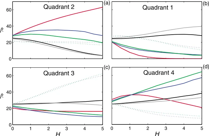
flows, which lack both homogeneity and isotropy. In order to demonstrate that homogeneous, isotropic turbulence (HIT) is different to environmental flows it is informative to contrast the results in Figure 1 with those in Figure 2 which are taken from the John Hopkins on-line turbulence data set for a direct numerical simulation of HIT using a 10243node simulation [Li et al., 2008]. Spatial series consisting of 1024 values are very short data sets compared to some of the others used in this paper and consequently, to obtain robust statistics we averaged our data over 100 different spatial series. That is a regular grid of 1010 points in thex z

plane was defined and the spatial series ofuywas extracted

for 1024 points along the y-axis. Our results are shown in Figure 2 and it is clear that the dependence of quadrant statistics onHdoes not exist in this case. Hence, the starting point of this paper that while the theory developed by

Kolmogorov [1941] may apply to HIT, it does not neces-sarily mean that it applies to other flows, appears to be borne out. This is reinforced by the additional flow types studied in sections 4 and 5.

4.

Flow Classification for Idealized Flow Types

[14] To extend the range of flow classes and to test the hypothesis from section 2 that for near-wall flows, as one moves away from the wall, the behavior in quadrant 1 increasingly departs from jet-like characteristics, we obtained nine velocity profiles at two different mean veloc-ities (U∞= 6 m s

1

andU∞= 8 m s 1

) in a horizontal, 1 m

cross-section wind tunnel with a 5 m measuring section located in a cold room at 15C described byKosugi et al.

[2004]. The surface was hydraulically rough consisting of snow grains with an average diameter of 3 mm, fixed in place by spraying them with water droplets and letting the water freeze. The longitudinal component of velocity was recorded at 5 kHz and 217 samples were recorded at each sampling point for each profile. The turbulence intensity

sðuÞ=u averaged 4.7 % for 6 m s 1and 5.0 % for 8 m s 1 inlet conditions at a height of 0.15 m from the wall (760 wall units,z+, forU∞= 6 m s

1

and 966z+forU∞= 8 m s 1

). Based on the wall unit scaling, the thickness of the viscous sublayer may be estimated to vary between 1 mm and 1.2 mm for the two input velocities. The Taylor Reynolds number at 0.15 m averaged 142 and 267 for the twoU∞and

Figure 3a shows that all profiles collapse appropriately using wall stress,u∗, scaling. Figures 3b–_{3e show the}

pro-portion of the data in each quadrant for H= 0 at various heights. It is important to note here the similarity of the results for the two different flow velocities and therefore, Reynolds numbers, which demonstrates that the results from our method are Reynolds number-independent.

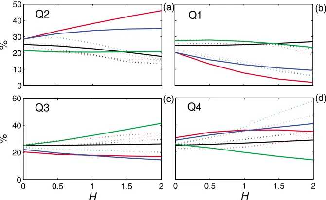
[15] The hypothesis from section 2 is borne out in Figure 3, where the flow close to the wall (Figures 3d and 3e) is rarely in Q1 relative toz≥0.1 m (Figures 3b and 3c) and this result holds for all nine individual experimental profiles. However, if we go further, and study the relative proportion of the data in each quadrant as a function ofH, important differences emerge as shown in Figure 4. In this figure we plot mean results for the wind tunnel experiments, as well as the jet data and measurements made in the far wake of a cylinder at inlet velocities ofU∞= 8.48 m s

1

and 24.3 m s 1[Stresing et al., 2010]. The means for the wind tunnel data were taken over the two measurements nearest the wall (z= 0.01 m,z= 0.02 m) and the two furthest from the wall (z= 0.12 m,z= 0.15 m) for the five experiments atU∞= 6 m s

1

and four atU∞= 8 m s 1

to give ten and eight measurements, respectively. It is clear that z affects the nature of the results in Figure 4 more than U∞ for the

wind tunnel data. The wake data are also more similar to each other than might be expected from differences inU∞.

Figure 2. Our quadrant analysis for homogeneous, isotro-pic turbulence taken from a direct numerical simulation. Note that the values are≈25% for all quadrants at all choices forH.

This supports our assertion about Reynolds number inde-pendence. The decrease in Q1 withHis strongest for the jet data, but is clearly seen near the wall and to a lesser extent further from the wall for the wind tunnel data. For these flows it is very rare to see fast flow where fluctuations are

suppressed. In contrast, results for the wake data are slightly increasing in Q1.

[16] While the hypothesis established in section 2, that jet data and flow near the wall would have a lack of events in quadrant 1, is borne out, jets and near-wall flows can readily

Figure 3. Boundary layer flow characteristics based on five experiments atU∞= 6 ms 1

(black lines) and four atU∞= 8 ms

1

(gray lines). (a) Dimensionless mean vertical velocity profiles using a wall units normalization, and (b–_{e) the distribution of time spent in different quadrants as a function of height above}

the snow surface for a hole size, H= 0.0. The bars indicate the range of results, with the central value showing the median. These bars are displaced slightly from the integer quadrant number for display purposes.

Figure 4. The relative proportion of events in each quadrant as a function of hole size,H.Thus, at any choice forH, the values for a particular data set over the four quadrants sum to 100%. The red line is the jet data while the black and gray lines are the wake data at 8.5 m s 1(black) and 24.3 m s 1(gray). The blue lines are the surface layer wind tunnel data atU_∞= 6 m s 1(blue) andU_∞= 8 m s 1(green). The solid line indicates the data near the wall, while the dotted lines are the sites closest to the center line of the wind tunnel.

KEYLOCK ET AL.: VELOCITY-INTERMITTENCY STRUCTURE F01037 F01037

be discriminated based on their behavior in other quadrants (particularly quadrants 2 and 4). The jet sees a relative increase in Q2 with H, which compensates for the decline in Q1 (and lesser decline in Q3 and Q4), while high in the wall flow it is Q3 that compensates for declines in Q1 and (strongly in) Q4. Close to the wall Q4 compensates for declines in Q1 and Q3, while the wake data also see increases in Q4 and Q1 to compensate for a clear decay in Q2. The pattern for jet flow was explained above, while the wall data can be explained with reference to near-wall turbulence structure [Adrian et al., 2000]. The faster flow near the wall is due to sweeps delivering fluid from a higher level in the flow where velocity fluctuations are more pronounced, resulting in a dominance of Q4. Higher up in the wall flow, the upward ejection of hairpin struc-tures with slower u than average at that z, but which are regions of concentrated vorticity, explains the dominance of Q3. At low H, the wake flow has a high proportion of slow moving, smooth flow from the near-wake region (Q2). As H increases this declines in importance relative to the fast, rough eddies that are generated by the shearing pro-cesses (Q4) and the occasional collapse of the recirculation region, with a downstream advection of fast, low turbulence fluid (Q1) [Simpson, 1989]. Because environmental fluid mechanics flows will often combine aspects of boundary-layer, wake and jet flows, the similarity between any real flow and the idealized cases reported here permits a flow classification to be undertaken. It is clear from these results than assuming an independence between velocity and the pointwise Hölder regularity and, thus, the increment struc-ture functions, is not appropriate for a wide range of non-isotropic flows and that this information provides a useful basis for flow classification.

5.

An Application to a Flume Study of a

Parallel-Channel Confluence

[17] The previous section of this manuscript demonstrated that idealized flow classes can be readily discriminated using our technique, which in turn calls into question the independence between velocity and Hölder structure for non-isotropic flows. Complex environmental flows may be classified as having some of the attributes of boundary-layer,

jet or wake flows depending on position and time. In this section of the paper we apply our method to data obtained from a parallel-channel confluence experiment undertaken in a 0.30 m wide flume over a rough bed of fixed sedimentary grains.

[18] The parallel-channel confluence was introduced by

Best and Roy [1991] as an end-member case for the flow dynamics at discordant river confluences. Because the junction angle is zero there is minimal momentum exchange between the flows and the dynamics of the confluence zone are driven by coherent flow structures that emerge from the interaction between two shear layers oriented at 90 to one another: the shear layer formed between the two incoming flows that induces vorticity in the longitudinal-transverse plane; the shear layer formed over the step of the discordant channel with vorticity in the longitudinal-vertical plane. The bed discordance reflects the fact that in natural channels there is often a significant sudden change in depth between the bed elevation of the smaller tributary and that of the main channel [Best and Ashworth, 1997]. Best and Roy [1991] noted that the coupling between the shear layers induces a fully three-dimensional flow structure, although large-eddy simulations byKeylock et al.[2005] showed that for a con-stant discharge ratio, the width of the discordant tributary plays an important role for the dynamics as a wider tributary reduces the pressure gradient between the recirculation zone behind the step and the rest of the flow, decoupling the two shear layers. There have been a number of additional experimental [Biron et al., 1996] and numerical [Bradbrook et al., 1998] studies of this particular flow geometry.

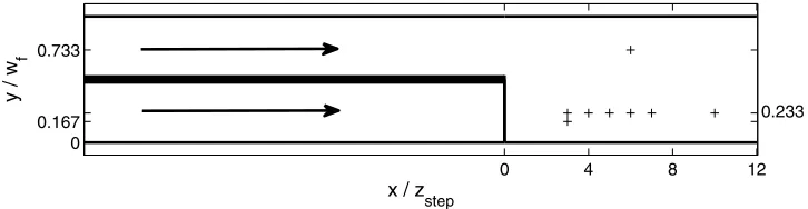
[19] The data used in this study were obtained in a hydraulic flume using an acoustic Doppler velocimeter, which recorded three perpendicular velocity components at 25 Hz. Data were obtained for 300 s from a sampling vol-ume with its base 1 median grain size (≈2.5 mm) above a fixed bed (sediment glued into position with 94 % of grains by mass with diameters in the 2.0 to 2.8 mm range) in the post-confluence region of the parallel-channel confluence. In this paper we consider the measurement sites in Figure 5, which represent a range of flow regimes (recirculation zone, impact of a shear layer, boundary-layer recovery). These are a small subset of all the measurements taken and the full set were used to delimit the recirculation region. The stratified

sampling strategy was determined on the basis of zones of sediment entrainment and deposition in similar experiments at the same velocity but using a mobile bed with the same sedimentary characteristics. The hydraulic flume had a width of 305 mm and a 9 mm splitter plate was placed along the center of the flume upstream of the confluence to partition the two flows, one of which passed over a step with a height,

zstep, of 50 mm. The flow depth in the raised channel was

70 mm and 120 mm in the unraised channel, with flow velocities of 0.55 m s 1 and 0.52 m s 1, respectively, meaning that the Reynolds number in both channels excee-ded 35 000 and the Froude number was less than 0.45. The data that are analyzed here were obtained along a transect in the post-confluence region but aligned with the center of the raised channel, as well as at a position largely unaffected by the flow dynamics of the shear layers (y/wf> 0.5), and one

close to reattachment where the flow is of a complex nature (x/zstep= 3.0,y/wf= 0.167), Figure 5. These data were

pre-viously used by Keylock[2009] to test a method for deter-mining the effective dimensionality of active periods [Keylock, 2008] in a turbulent flow field.

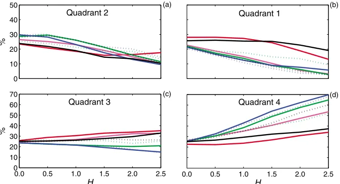
[20] Our results are given in Figure 6 where, as the colors change from green, to blue, to black, one moves further along the transect, away from separation (x/zstep ∈

{3, 4, 5, 6,, 7, 10}, y/wf = 0.233) and where the red

and magenta lines are for (x/zstep = 6.0,y/wf= 0.733) and

(x/zstep = 3.0, y/wf = 0.167), respectively. The results are

truncated at H = 2.5, compared to H = 5.0 in Figure 4 because of the much shorter duration of the record, which means that there are too few data beyond this H

for significant conclusions to be drawn. Note that at (x/zstep= 3.0,y/wf= 0.167) and (x/zstep= 3.0,y/wf= 0.233)

the measurements are within the recirculation zone and the mean value for ux is negative. Consequently, in order to

compare these data to the others, the results from quad-rants 1 and 2, and then quadquad-rants 3 and 4, were trans-posed. Some of the flows in Figure 4 and various sites in

Figure 6 show similar behavior. To facilitate a comparison between these cases, selected data from Figure 4 and Figure 6 are plotted together in Figure 7.

[21] It is clear in Figure 6b and 6d in particular, that the flows that are least affected by separation processes (the black line where x/zstep = 10 and the red line where y/wf> 0.7) have a different response to the other sites and

their gradual rise in quadrant 4 together with decay in quadrant 2 and a fairly constant response in quadrant 3 is, from Figure 4 and Figure 7, indicative of a far-wake flow field, although the response in quadrant 1 is also similar to flow high in the near-wall flow. At these two locations the flow is primarily described by boundary-layer recovery interspersed with periodic shedding of slow fluid from the recirculation region behind the step, which is borne out by the results. The shedding of structures in the lee of the obstacle is what explains the opposite response of the far-wake data to the jet data in Figure 4 (less turbulent recir-culation zone flow immersed in a more turbulent flow compared to highly turbulent flow injected into a quiescent fluid) and our results imply that the shedding of the recir-culation zone has similar effects as in far-wake situations.

[22] The sites at (x/zstep ∈ {4, 5, 6,, 7}, y/wf = 0.233)

largely exhibit a similar response to one another that for quadrant 1 is akin to the blue and green lines in Figure 4 (blue line in Figure 7) for near wall data, while the behav-ior in quadrants 2 and 3 is intermediate between near-wall and wake cases and the rise in quadrant 4 is greater than seen in even the near-wall flow. Given that these measurements were made near the wall and are affected by the wake shedding processes that affect (x/zstep = 10, y/wf = 0.233)

this behavior is not unsurprising. In particular, the coinci-dence of wake shedding and energetic Kelvin-Helmholtz eddies in the confluence explains the dominance of quad-rant 4 at high H relative to other quadquad-rants as well as to near-wall flows affected largely by less energetic hairpin

Figure 6. The relative proportion of events in each quadrant as a function of hole size,H, for the conflu-ence experiment. The lines in each plot correspond to data from different sites in the post-confluconflu-ence region: (x/zstep= 6.0,y/wf= 0.733) red, (x/zstep= 3.0,y/wf= 0.167) magenta, (x/zstep= 3.0,y/wf= 0.233)

green dotted, (x/zstep= 4.0,y/wf= 0.233) green, (x/zstep= 5.0,y/wf= 0.233) blue dotted, (x/zstep= 6.0, y/wf = 0.233) blue, (x/zstep = 7.0, y/wf = 0.233) black dotted, (x/zstep = 10.0, y/wf = 0.233) black.

KEYLOCK ET AL.: VELOCITY-INTERMITTENCY STRUCTURE F01037 F01037

vortex formation and corresponding sweeps. Hence, these sites seem to be different to, but related to near-wall flow.

[23] The recirculation region (magenta line in Figure 6) appears to have rather different characteristics even after the sign change. In quadrants 1 and 4 it behaves like the near-wall cases, while in quadrants 3 and 4 it is nearer the far-wake cases. It should be noted that none of the idealized flow types in Figure 4 covered this case and its status as a distinct case is to be expected.

[24] The lack of an increase in percentage occupancy withHin quadrant 2, coupled to increases in quadrant 4 for the sites in Figure 6 would suggest that, when compared to the red line in Figure 3, the jet model is inappropriate for the post-confluence flow as one might expect. That none of the sites, which are subject to a variety of forms of vortex impingement seem to exhibit characteristics of the jet data cautions against the use of jet data as a model for sediment transport by coherent flow structures in environmental flows [Hogg et al., 1996].

[25] This application of our method appears to be suc-cessful. The sites furthest from the region of coherent structure impingement upon the bed, which are mainly subject to the advected remnants of these structures appear to have similar characteristics to far-wake flows. On the other hand, flow near a lower boundary that is suddenly subject to major reorganizations as structures impose upon the bed, are similar to near-wall boundary layer flows. There is perhaps no clear analogue for flow in a recirculation zone from the fluid mechanics data analyzed in section 4 and it is at these sites where the behavior differs most markedly from the analogues in Figure 4. As discussed bySimpson[1989] recirculation zones are not regions of quiescent flow but the effect of intermittency-driven-by-impingement will be dampened compared to a near-wall boundary layer flow or a region where structures are directly impinging upon the bed,

explaining the observed characteristics that are more similar to a far wake.

6.

Implications for Sediment Transport

[26] While the mobilization of particles into suspension is largely a function of the strength of ejections (upward movements of relatively slow moving fluid from the wall), bed load entrainment is coupled tou/> 0, largely driven by the dominant action of sweeps, although the rarer outward inter-actions are more efficient [Heathershaw and Thorne, 1985;

Nelson et al., 1995]. Recently there has been an increased understanding of the role of impulse rather than instantaneous maximum forces for particle entrainment [Diplas et al., 2008;

Valyrakis et al., 2010], with some particles transported when

u/> 0 for a sustained period but peak stresses are relatively low. Sustaining u/ > 0 for a significant period implies that

ap/ > 0. Figures 1, 3, and 4 show that for jet flows and

boundary layer flows, the joint probability of fast, smooth (Q1) events is relatively low, meaning that in the natural environ-ment, for a well-developed boundary layer, impulse-based considerations, while important, will be potentially out-weighed by the effect of higheru/flow events whereap/ < 0

and the flow event is of limited duration. However, when considering flow in complex environments, such as gravel bed rivers where vortex shedding from individual clasts occurs [Hardy et al., 2007] or where the form resistance from the bed disrupts the classical boundary layer [Venditti et al., 2005], the flow is more likely to behave as the wake flow (gray and black lines in Figure 4 and the far-field locations from the parallel-channel confluence experiment in Figure 6). In which case, Q1 is of much greater importance and we can expect that impulse-based considerations are of greater relevance for elucidating bed load sediment entrainment. Hence, our flow classification scheme, which appears to have been successfully applied to

Figure 7. The relative proportion of events in each quadrant as a function of hole size,H, for selected data from Figure 4 and Figure 6: jet data (red), the 8.5 m s 1wake data (black), the surface layer wind tunnel data near the bed atU_∞= 6 m s 1(blue), the surface layer wind tunnel data high in the flow at

U∞= 6 m s 1

(green), confluence sites (x/zstep= 6.0,y/wf= 0.733) red dotted, (x/zstep= 3.0,y/wf= 0.167)

the case of near-bed flow in a complex environment, can be used to infer the importance of the recent, exciting develop-ments in bed-load entrainment studies. Elucidating this con-nection explicitly will be the topic of future research.

7.

Conclusion

[27] A method for studying the coupling between turbu-lent fluctuating velocities and their pointwise Hölder expo-nents has been presented. This method can successfully discriminate between various classes of turbulent flow in a manner that agrees with knowledge of the relevant dynam-ics. Because the differences between flow types dominates variation in Reynolds number, our method would appear to be robust to variation in mean velocity. The technique demonstrates the presence of a coupling between velocities and the intermittency in different flows and provides a means for classifying environmental turbulence flows. Based on this method, it would seem that the recently pro-posed ideas concerning impulse-based bed load sediment entrainment are primarily relevant in rough boundaries, where the boundary-layer structure is disrupted such that much of the near-wall flow can be considered to behave as a far-wake flow.

Appendix A: Hölder Exponents and Their Relation

to Velocity Increments

[28] The main part of this paper develops a method for the visual analysis of turbulence signals based on the depen-dence between the fluctuating longitudinal velocity and the fluctuating series of Hölder exponents for the data, where a Hölder exponent may be thought of as a pointwise estimate of the fractal dimension of the signal. In this appendix we develop a connection between the structure functions given by different choices for nin equation (1) and the value for Hölder exponents. Thus, we show that the analysis devel-oped here is related to those that directly study velocity increments [Hosokawa, 2007;Stresing and Peinke, 2010].

[29] The structure function approach was developed by

Frisch and Parisi [1985] as shown in equation (1) and the top line of equation (A3). Given a power law scaling between the moments of the velocity increments, vr, and

their separation, r, denoted by xn, a monofractal signal

will exhibit a linear scaling between the moment order,n, and

xn as seen in Kolmogorov’s original theory [Kolmogorov,

1941], while a multifractal signal will exhibit a convex rela-tion between n, and xn [Frisch and Parisi, 1985]. Thus,

a connection between the velocity increments and the fractal or multifractal nature of a velocity signal can be demonstrated.

[30] Given the definition of the Hölder exponent in equation (5), multifractal analysis is concerned with the study of the sets Sa, where a function has a given Hölder

exponent, a. If for eacha, we define the singularity spec-trum, D(a) as the set of values for a for which Sa is not

empty. The Frisch-Parisi conjecture states that

DðaÞ ¼min

n ðan xnþ1Þ ðA1Þ

That is, the structure functions and the Hölder exponents are related via a Legendre transform. Hence, the analysis in this

paper based on Hölder exponents is intimately connected to structure functions and, thus, velocity increments. To make this more explicit and following Jaffard[1997], if we are close to a singularity of ordera, we will find that in a win-dow, |r|, that the local behavior scales as

uxþr uxjn≈jrjan

j ðA2Þ

With a dimension to these singularities of D(a) it follows that there are approximately |r| D(a) boxes with a volume |r|mwherem is the dimension of the space over which the function is defined. Hence, the contribution of this singu-larity to the integral used to evaluate the structure function

〈_|vr|n_〉

is approximately |r|an + m D(a). The largest con-tributor to the integral will be given by the smallest expo-nent becauser→0. Thus,

hjvrj in ∝jrxn

ðA3Þ

x_n¼min

n ðan DðaÞ þmÞ ðA4Þ

This derivation gives the link between the scaling behavior of the structure functions and the spectrum of Hölder exponents. However, usually we knowxnand are trying to

estimateD(a). Thus, we need to take the inverse Legendre transform, which for a m = 1 dimensional signal yields equation (A1).

[31] Acknowledgments. We are grateful to Robert Stresing for his assistance with and comments on this work and to Christos Vassilicos for providing a forum for discussion. C.J.K. acknowledges his short-term fellowship from the Japan Society for the Promotion of Science (PE04511) hosted by K.N. and the Nagaoka Institute for Snow and Ice Studies.

References

Adrian, R. J., C. D. Meinhart, and C. D. Tomkins (2000), Vortex organiza-tion in the outer region of the turbulent boundary layer,J. Fluid Mech.,

422, 1–_54.

Best, J. L. (1992), On the entrainment of sediment and the initiation of bed defects: Insights from recent developments within turbulent boundary layer research,Sedimentology,39, 797–_811.

Best, J. L., and P. J. Ashworth (1997), Scour in large braided rivers and the recognition of sequence stratigraphic boundaries,Nature,387, 275–277. Best, J. L., and A. G. Roy (1991), Mixing layer distortion at the confluence

of channels of different depth,Nature,350, 411–_413.

Biron, P., A. G. Roy, and J. L. Best (1996), Turbulent flow structure at concordant and discordant open-channel confluences, Exp. Fluids,21, 437–_446.

Bogard, D. G., and W. G. Tiederman (1986), Burst detection with single-point velocity measurements,J. Fluid Mech.,162, 389–_413.

Bradbrook, K. F., P. M. Biron, S. N. Lane, K. S. Richards, and A. G. Roy (1998), Investigation of controls on secondary circulation in a simple con-fluence geometry using a three-dimensional numerical model, Hydrol. Processes,12, 1371–_1396.

Diplas, P., C. L. Dancey, A. O. Celik, M. Valyrakis, K. Greer, and T. Akar (2008), The role of impulse on the initiation of particle movement under turbulent flow conditions,Science,322, 717–_720.

Friedrich, R., and J. Peinke (1997), Description of the turbulent cascade by a Fokker-Planck equation,Phys. Rev. Lett.,78, 863–_866.

Frisch, U., and G. Parisi (1985), The singularity structure of fully developed turbulence, in Turbulence and Predictability in Geophysical Fluid Dynamics and Climate Dynamics, edited by M. Ghil, R. Benzi, and G. Parisi, pp. 84–88, Elsevier, New York.

Hardy, R. J., S. N. Lane, R. I. Ferguson, and D. R. Parsons (2007), Emer-gence of coherent flow structures over a gravel surface: A numerical experiment, Water Resour. Res., 43, W03422, doi:10.1029/ 2006WR004936.

Heathershaw, A. D., and P. D. Thorne (1985), Sea-bed noises reveal role of turbulent bursting phenomenon in sediment transport by tidal currents,

Nature,316, 339–_342.

KEYLOCK ET AL.: VELOCITY-INTERMITTENCY STRUCTURE F01037 F01037

Hogg, A. J., W. B. Dade, H. E. Huppert, and R. L. Soulsby (1996), A model of an impinging jet on a granular bed, with application to turbulent, event-driven bed load transport, inCoherent Flow Structures in Open Chan-nels, edited by P. J. Ashworth et al., pp. 101–_{124, John Wiley, New York.}

Hosokawa, I. (2002), Markov process built in scale-similar multifractal energy cascades in turbulence,Phys. Rev. E,65, 027301, doi:10.1103/ PhysRevE.65.027301.

Hosokawa, I. (2007), A paradox concerning the refined similarity hypothe-sis of Kolmogorov for isotropic turbulence, Prog. Theor. Phys.,118, 169–_173.

Jaffard, S. (1997), Multifractal formalism for functions Part 1. Results valid for all functions,SIAM J. Math. Anal.,28, 944–_970.

Kahalerras, H., Y. Malécot, Y. Gagne, and B. Castaing (2007), Intermit-tency and Reynolds number,Phys. Fluids,10, 910–_921.

Katul, G., H. Cheng, G. Kuhn, D. Ellsworth, and D. Nie (1997), Turbulent eddy motion at the forest-atmosphere interface,J. Geophys. Res.,102, 13,409–_13,421.

Keylock, C. J. (2007), The visualization of turbulence data using a wavelet-based method,Earth Surf. Processes Landforms,32, 637–_647.

Keylock, C. J. (2008), A criterion for delimiting active periods within turbulent flows, Geophys. Res. Lett., 35, L11804, doi:10.1029/ 2008GL033858.

Keylock, C. J. (2009), Evaluating the dimensionality and significance of active periods in turbulent environmental flows defined using Lipshitz/ Hölder regularity,Environ. Fluid Mech.,9, 509–523.

Keylock, C. J. (2010), Characterizing the structure of nonlinear systems using gradual wavelet reconstruction, Nonlinear Processes Geophys.,

17, 615–632.

Keylock, C. J., R. J. Hardy, D. R. Parsons, R. I. Ferguson, S. N. Lane, and K. S. Richards (2005), The theoretical foundations and potential for large-eddy simulation (LES) in fluvial geomorphic and sedimentological research,Earth Sci. Rev.,71, 271–_304.

Kolmogorov, A. N. (1941), The local structure of turbulence in incompress-ible viscous fluid for very large Reynolds numbers,Dokl. Akad. Nauk. SSSR.,30, 299–303.

Kolmogorov, A. N. (1962), A refinement of previous hypotheses concerning the local structure of turbulence in a viscous, incompressible fluid at high Reynolds number,J. Fluid Mech.,13, 82–85.

Kolwankar, K. M., and J. Lévy Véhel (2002), A time domain characteriza-tion of the fine local regularity of funccharacteriza-tions,J. Fourier Anal. Appl.,8, 319–_334.

Kosugi, K., T. Sato, and A. Sato (2004), Dependence of drifting snow saltation lengths on snow surface hardness,Cold Reg. Sci. Tech.,39, 133–_139.

Li, Y., E. Perlman, M. Wan, Y. Yang, R. Burns, C. Meneveau, S. Chen, A. Szalay, and G. Eyink (2008), A public turbulence database cluster and applications to study Lagrangian evolution of velocity increments in turbulence,J. Turbulence,9, 1–29.

Lovejoy, S., A. F. Tuck, S. J. Hovde, and D. Schertzer (2007), Is isotropic turbulence relevant in the atmosphere?,Geophys. Res. Lett.,34, L15802, doi:10.1029/2007GL029359.

Lu, S. S., and W. W. Willmarth (1973), Measurements of the structure of the Reynolds stress in a turbulent boundary layer,J. Fluid Mech.,60, 481–_511.

Luchik, T. S., and W. G. Tiederman (1987), Timescale and structure of ejections and bursts in turbulent channel flows, J. Fluid Mech., 174, 529–_552.

Meneveau, C., and K. Sreenivasan (1991), The multifractal nature of turbu-lent energy-dissipation,J. Fluid Mech.,224, 429–_484.

Muzy, J. F., E. Bacry, and A. Arnéodo (1991), Wavelets and multifractal formalism for singular signals: Application to turbulence data, Phys. Rev. Lett.,67, 3515–3518.

Nakagawa, H., and I. Nezu (1977), Prediction of the contributions to the Reynolds stress from bursting events in open channel flows,J. Fluid Mech.,80, 99–_128.

Nelson, J. M., R. L. Shreve, S. R. McLean, and T. G. Drake (1995), Role of near-bed turbulence in bed-load transport and bed form mechanics,Water Resour. Res.,31, 2071–_2086.

Niño, Y., and M. Garcia (1996), Experiments on particle-turbulence interac-tions in the near-wall region of an open channel flow: Implicainterac-tions for sediment transport,J. Fluid Mech.,326, 285–_319.

Praskovsky, A. A., E. B. Gledzer, M. Y. Karyakin, and Y. Zhou (1993), The sweeping decorrelation hypothesis and energy-inertial scale interac-tion in high Reynolds number flow,J. Fluid Mech.,248, 493–_511.

Renner, C., J. Peinke, and R. Friedrich (2001), Experimental indications for Markov properties of small-scale turbulence, J. Fluid Mech., 433, 383–_409.

Seuret, S., and J. Lévy Véhel (2003) A time domain characterization of 2-microlocal spaces,J. Fourier Anal. Appl.,9, 473–495.

She, Z., and E. Leveque (1994), Universal scaling laws in fully developed turbulence,Phys. Rev. Lett.,72, 336–_339.

Simpson, R. L. (1989), Turbulent boundary-layer separation,Ann. Rev. Fluid Mech.,21, 205–_234.

Sreenivasan, K. R., and G. Stolovitzky (1996), Statistical dependence of inertial range properties on large scales in a high-Reynolds-number shear flow,Phys. Rev. Lett.,77, 2218–_2221.

Stresing, R., and J. Peinke (2010), Towards a stochastic multi-point descrip-tion of turbulence,New J. Phys.,12, 103046, doi:10.1088/1367-2630/12/ 10/103046.

Stresing, R., J. Peinke, S. Seoud, and J. Vassilicos (2010), Defining a new class of turbulent flows, Phys. Rev. Lett., 104, 194501, doi:10.1103/ PhysRevLett.104.194501.

Valyrakis, M., P. Diplas, C. L. Dancey, K. Greer, and A. O. Celik (2010), Role of instantaneous force magnitude and duration on particle entrain-ment,J. Geophys. Res.,115, F02006, doi:10.1029/2008JF001247. Venditti, J. G., M. A. Church, and S. J. Bennett (2005), Bed form initiation

from a flat sand bed, J. Geophys. Res., 110, F01009, doi:10.1029/ 2004JF000149.

C. J. Keylock, Department of Civil and Structural Engineering, University of Sheffield, Mappin Bldg., Mappin St., Sheffield S1 3JD, UK. ([email protected])

K. Nishimura, Graduate School of Environmental Studies, Nagoya University, Furo-cho, Chikusa-ku, Nagoya 464-8601, Japan. (knishi@ nagoya-u.jp)