Spatial localization in heterogeneous systems

Spatial localization in heterogeneous systems

Hsien-Ching Kao*

Wolfram Research Inc., Champaign, Illinois 61820, USA

C´edric Beaume†and Edgar Knobloch‡

Department of Physics, University of California, Berkeley, California 94720, USA (Received 18 October 2013; published 6 January 2014)

We study spatial localization in the generalized Swift-Hohenberg equation with either quadratic-cubic or cubic-quintic nonlinearity subject to spatially heterogeneous forcing. Different types of forcing (sinusoidal or Gaussian) with different spatial scales are considered and the corresponding localized snaking structures are computed. The results indicate that spatial heterogeneity exerts a significant influence on the location of spatially localized structures in both parameter space and physical space, and on their stability properties. The results are expected to assist in the interpretation of experiments on localized structures where departures from spatial homogeneity are generally unavoidable.

DOI:10.1103/PhysRevE.89.012903 PACS number(s): 82.40.Ck,47.54.−r,47.20.Ky,47.55.P−

I. INTRODUCTION

A large variety of physical systems exhibits stationary spatially localized structures in appropriate parameter regimes. These include different convective systems driven by an imposed temperature difference [1–7], a ferrofluid subject to an imposed magnetic field [8] and an optical light valve experiment driven by a nominally uniform light intensity [9]. Other systems exhibiting localized structures include shear flows [10,11], gas discharges [12], and a variety of optical con-figurations [13,14]. In modeling these systems one typically as-sumes that the forcing of the system is spatially homogeneous, be it the imposed temperature difference across a convection system or the magnetic field imposed across a ferrofluid. In experiments, however, spatial homogeneity is difficult if not impossible to achieve. Spatial heterogeneities arise from a variety of sources, including edge or sidewall effects, imperfect temperature control, magnetic field perturbations, and a variety of topographic effects such as surface imperfections that are usually assumed to be absent. Lateral parameter gradients generally lead to drift [15] and trapping of structures by spatial heterogeneities in the gradients. In the present work we study the steady structures created by these processes with a view to gaining a solid understanding of the effects of spatial hetero-geneities on the presence and stability of stationary localized structures. We show, in particular, that spatial heterogeneities may, under appropriate conditions, substantially modify the standard homoclinic snaking scenario [16] that has been so successful in interpreting the results of numerical simulations of nominally one-dimensional systems [4,17].

The Swift-Hohenberg equation has played a fundamental role in our understanding of homogeneous systems, serving as a “normal form” for systems undergoing a steady-state insta-bility with a finite wave number at onset. The reason for this is that in one spatial dimension the basic snakes-and-ladders structure [18] of the so-called snaking or pinning region in

*_{[email protected]}

†_{[email protected]} ‡_{[email protected]}

parameter space that organizes the localized structures in two or four intertwined solution branches is generated by transversal intersections of certain manifolds [19,20]. Such intersections are structurally stable with respect to sufficiently small changes in the equation such as changes in the parameter values or in the form of the nonlinearity. The equation takes the form

ut =au−(1+∂xx)2u+N(u), (1)

where u(x,t) is a scalar order parameter, x and t denote space and time variables, and N(u) is a smooth nonlinear function. The parametera represents forcing, with the trivial stateu=0 stable fora <0 and unstable fora >0. Note that x has been scaled so that the primary instability corresponds to wave numberk=1. With periodic boundary conditions on the spatial domain [−/2,/2], Eq. (1) exhibits variational dynamics with the Lyapunov functional (or free energy)

F ≡ /2

−/2

−1 2au

2₊1

2[(1+∂xx)u]

2₋ u

0

N(v)dv

dx.

(2)

This property implies that any initial condition integrated forward in time tends, as time increases, to either a stationary state or a front propagating at constant speed. We define the

Maxwell pointas the value of the parameterafor whichF =0 along the branch of spatially periodic solutions emerging from the primary instability ata =0. At this value ofathe periodic state with wave number k=1 has the same free energy as the trivial state u=0. Two choices of N(u) have proved particularly useful:

N₂₃(u)≡1.8u2−u3, (3)

N35(u)≡2u3−u5. (4)

bex=0, i.e., under the operation

R₁:x→ −x, u→u.

The choiceN35introduces the additional symmetry

R2:x→x, u→ −u.

This symmetry is appropriate for modeling physical systems with midplane reflection symmetry such as Boussinesq con-vection or plane Couette flow.

In the following we generalize the Swift–Hohenberg equation and incorporate spatially heterogeneous conditions by allowing the parametera to depend on x. This assump-tion destroys the translaassump-tion invariance and selects preferred locations in space for the localized structures that remain. Of course translation invariance may be broken in any number of different ways (the translation invariant problem is formally of infinite codimension), but we choose here two representative forcing profiles, a=a(x)≡r[1+αf(x)], where f(x) is either periodic with period 2π/δor Gaussian with widthσ:

fp(x)≡cos(δx), fb(x)≡exp(−x2/2σ2). (5)

The periodic heterogeneity fp corresponds to a sinusoidal forcing with mean r, relative oscillation amplitude α, and wave numberδ. The caseδ=1 corresponds to a 1:1 resonance between the wave number of the forcing and that intrinsic to the Swift–Hohenberg equation. The bump heterogeneity fb models homogeneous forcing locally perturbed by a bell-like departure. In this case, the background forcing has amplitude r and the bump is modeled using a Gaussian function of amplitudeαand width proportional toσ.

In the following sections, we report results on the location and stability of localized structures in the presence of the heterogeneities fp and fb with different spatial scales and amplitude. The numerical continuation package AUTO [21] is used to follow solutions in a domain of spatial extent=40π, a length sufficiently large (20 times the critical wavelength) to allow spatial localization. Owing to the choice of forcing, the system is spatially reversible with respect tox=0 and we carry out our computations on the half-domain [0,/2]. The solutions for SH23 are computed using Neumann boundary conditions

ux =uxxx=0 (6)

atx =0,/2 and then reflected inx=0 to obtain solutions on the full domain. For SH35, this procedure yields only solutions with even parity. To find solutions with odd parity we impose Dirichlet boundary conditions

u=uxx =0 (7)

at x=0,/2 and use the symmetry R1◦R2 to extend the

solution to the full domain. In all cases we show bifurcation diagrams in terms of theL2norm of the solution, defined as

uL2≡

1

/2

−/2 u2dx

1/2

. (8)

In the following section, we recall the basic results for the formation of localized structures in the Swift-Hohenberg equation with homogeneous forcing. In Sec.III we present results obtained when a periodic heterogeneity with O(1)

length scale is turned on, i.e., when the length scale of the heterogeneity is comparable to the natural length scale of the problem. SectionIVis devoted to the stability properties of the solutions subject to heterogeneous forcing. SectionV

presents results for heterogeneities that vary on the scale O(), i.e., on the scale of the domain size, with 1. In each case we examine the effects of periodic forcing with the requisite scale and compare it with the effects of an isolated Gaussian bump with a comparable length scale. In Sec. VI we determine the displacement of the saddle nodes of the competing periodic branches through an analytical calculation, followed in Sec.VIIby an investigation of temporal dynamics of spatially localized patterns in the presence of heterogeneous forcing. The paper concludes with a summary of the results together with a discussion of their implications for experiments.

II. HOMOGENEOUS FORCING

The homogeneous one-dimensional Swift–Hohenberg equation has been the focus of a number of recent stud-ies [16,18,20,22] and the formation of localized structures in one spatial dimension within this equation is now well understood. Here we provide a brief overview of known results for SH23 and SH35 that will be used for comparison with the new results in the following sections. The results in the presence of homogeneous forcing for SH23 and SH35 are reported in Figs.1and2, respectively. The trivial solution first becomes unstable at r =0 due to a subcritical bifurcation. This bifurcation creates a one-parameter family of spatially periodic states of wavelength 2π. At each r we select two representatives from this family. In SH23 one of the solutions has a peak atx=0 (hereafterφ=0, black curve), while the other has a trough at x=0 [hereafter φ=π, red (or gray) curve]. Both are of even parity. In SH35 these solutions are related by the additionalR2symmetry and are both represented

in black. However, one also has odd solutions withu|x=0 =0

and either a positive (φ=π/2) or a negative (φ=3π/2) slope atx=0. These solutions are referred to as odd parity solutions and are represented in red (or gray). This color convention will be used throughout the remainder of this paper. In both cases, the spatially periodic branches undergo saddle node bifurcations before turning towards larger values of r and hence larger amplitudes. Owing to the finite size of the domain, a modulational instability occurs along these branches at small but nonzero amplitude [23] generating two distinct branches of localized states: theφ=0 andφ=π branches in SH23, and two even (φ=0,π) and two odd (φ=π/2,3π/2) branches in SH35, each arising from modulational instability occurring along the periodic solutions of the appropriate phase. All these localized branches exhibit back-and-forth oscillations within a well-defined parameter interval in a behavior known as homoclinic snaking [19]. These oscillations reflect the nucleation of additional oscillations in the solution profile at the locations of the fronts bounding the structure, as described in greater detail in Ref. [18], resulting in the growth of the structure and hence increasedL2norm. In SH23 the solution

−0.4 −0.3 −0.2 −0.1 0 0

0.2 0.4 0.6 0.8 1

r

N

(a)

−60 −40 −20 0 20 40 60

(b)

x

FIG. 1. (Color online) (a) Bifurcation diagram showing N≡ uL2as a function ofrfor homogeneous forcing (α=0) in SH23. The black [red (or gray)] snaking branch corresponds to solutions withφ=0 (φ=π). (b) Solution profiles at the bottom five saddle nodes along each snaking branch. The asymmetric rung states [22] are omitted.

solution adds half of an oscillation (either a peak or a trough) between every second saddle node implying that the frequency of the back-and-forth oscillations of the branch is doubled. Once the branch of localized states exits the snaking region it reconnects with the original periodic branch near its saddle node. During the snaking, all the branches of localized states experience alternating stability and instability as the amplitude eigenvalue oscillates through zero at successive saddle nodes. As a result the segments of each branch connecting the saddle nodes from left to right (proceeding upwards) are stable and the rest is unstable. The resulting diagrams constitute reference results for the subsequent sections on spatially dependent forcing.

We mention that the branches of even states in SH23 are connected by a series of rungs consisting of asymmetric states, forming a snakes-and-ladders structure [22]. Similar rungs connect even and odd states in SH35 [16,18]. All are unstable, but will be found to play a significant role onceα=0.

III. HETEROGENEOUS FORCING ON AO(1) SPATIAL SCALE

In this section we examine the effects of spatially periodic forcing on aO(1) spatial scale. The values of the parameters

−1 −0.8 −0.6 −0.4 −0.2 0

0 0.2 0.4 0.6 0.8 1 1.2

r

N

(a)

−60 −40 −20 0 20 40 60

(b)

x

FIG. 2. (Color online) (a) Bifurcation diagram showing N≡ uL2as a function ofrfor homogeneous forcing (α=0) in SH35. The black [red (or gray)] snaking branch corresponds to even (odd) solutions. (b) Solution profiles at the bottom five saddle nodes along the left end of the snaking branches. The asymmetric rung states [18] are omitted.

areδ=1 for the periodic heterogeneityfp andσ =π/2 for the bump heterogeneityfb.

A. Periodic heterogeneity fp

−0.4 −0.3 −0.2 −0.1 0 0

0.2 0.4 0.6 0.8 1

r

N

(a)

−0.4 −0.3 −0.2 −0.1 0

0 0.2 0.4 0.6 0.8 1

r

N

(b)

FIG. 3. (Color online) Bifurcation diagrams for SH23 with the forcingfp and δ=1, showingN≡ uL2 as a function of r for (a) φ=0 steady states and (b) φ=πsteady states. The forcing amplitudeα=0.1 (solid lines) andα= −0.1 (dashed lines).

region of the φ=πlocalized states. The associated snaking behavior is much more complex and a partial snaking branch (solid black curve) is shown in Fig. 3(b). When α <0 the results are similar but not identical. The change of sign ofα amounts to a translation of the forcing by half a period, and we use the label φ=0 ( φ=π) to refer to solutions whose maxima (minima) are again in phase with the forcing maxima. The corresponding localized states are shown in Figs.3(a)and 3(b) using dashed lines. As forα >0, the resulting φ=0 snaking branch is complete and resembles in all respects the φ=0 snaking branch in SH23 with homogeneous forcing (Fig.1). This is no longer the case for the φ=πlocalized states [Fig.3(b)].

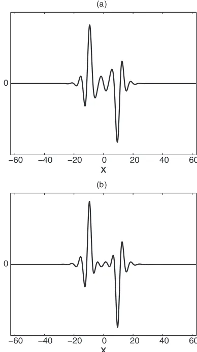
Figure 4 shows profiles of the localized solutions with φ=πfor (a)α=0.1 and (b)α= −0.1 [Fig.3(b)]. In both cases the snaking is incomplete: theα=0.1 (resp.α= −0.1) φ=π branch snakes normally until a 7- (resp. 8-) peak solution is reached but then doubles back and starts to snake towards states with a lowerL₂ norm. As it does so, a defect is created that flattens the central region creating a state reminiscent of a two-pulse state [5,24]. The resulting behavior resembles that of localized structures in SH23 on nonperiodic domains with mixed boundary conditions [25,26].

A reliable guide to the shift of the snaking regions for the φ=0 and φ=πsteady states is obtained by tracking the

−60 −40 −20 0 20 40 60

(a)

x

−60 −40 −20 0 20 40 60

(b)

x

FIG. 4. (Color online) Solution profiles at successive saddle nodes along the φ=πbranches from Fig.3(b)for (a)α=0.1 and (b)α= −0.1, proceeding upward along the branch (profiles below the horizontal separation line) and then following it further as it starts to snake back down (profiles above the horizontal separation line). The bottom panel shows the forcing functionfp(thin solid line).

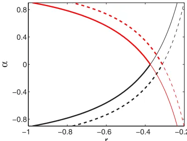
motion of the saddle node of the periodic states and of the Maxwell point as a function of the amplitudeαof the forcing fp. Figure5shows the result. Whenα=0 the saddle nodes of the φ=0,πperiodic states coincide as do the corresponding Maxwell points, with the latter to the right of the former. As|α| increases both points move to the left for solutions of φ=0 type (thick lines) but to the right for solutions of φ=π type (thin lines). Thus the snaking regions for the φ=0 and φ=π solutions are pulled apart and ultimately do not overlap at all.

−1 −0.8 −0.6 −0.4 −0.2 −0.8

−0.4 0 0.4 0.8

r

α

FIG. 5. (Color online) Location of the saddle nodes of the peri-odic branches (solid lines) and the associated Maxwell points (dashed lines) in the (r,α) plane for SH23. The thick (thin) lines represent φ=0 ( φ=π) solutions.

gradual erosion of a peak at the right of the structure, resulting in an overall translation of the symmetry point from x=0 tox= −π. Similar transitions have been observed in integral models for neural fields where the rung states grow on one side while remaining pinned [27]. Such solutions can be translated

−0.36 −0.32 −0.28

0.35 0.39 0.43

r

N

(a)

−60 −40 −20 0 20 40 60

(b)

x

FIG. 6. (Color online) (a) Bifurcation diagrams for SH23 with the forcingfpandδ=1, showingN≡ uL2as a function ofrfor φ=0 steady states. The forcing amplitudeα=0.1 (solid lines) and α= −0.1 (dashed lines). Dash-dotted lines: rung states. (b) Sample solution profiles along the lower rung branch in (a) from left (bottom) to right (top).

back to x =0 by translating the heterogeneity fp by π to the right. Since the translation of fp by π is equivalent to changing the sign ofαit follows that such rung states connect symmetric states with opposite signs of the forcing amplitude α as indicated in Fig. 6(a). The resulting rungs are omitted from Fig.3(a)for clarity.

The bifurcation diagrams obtained with cubic-quintic non-linearity are shown in Figs. 7 and 8 for which we chose α= ±0.1 andα= ±0.5. As mentioned in Sec.II, there are two types of solutions: those with even parity with respect to the center x =0 (Fig. 7) and those with the odd parity with respect to the same point (Fig.8). Note that we do not have to distinguish between even solutions with maxima that are in phase with the forcing ( φ=0) and that are π out of phase ( φ=π) since these are related by the symmetry (u,f)→ −(u,f) and likewise for odd solutions with positive (negative) slope at the location of maxima in the forcing ( φ= ±π/2).

For even parity localized structures, the full snaking structure persists and the snaking region broadens as |α| increases. At the same time the two-limit snaking familiar from the homogeneous case turns into four-limit snaking: for α >0 this leads to successive saddle nodes at locations r1→r4→r2→r3→r1· · ·, while forα <0 the sequence

is r2→r3→r1→r4→r2· · ·. Here ri < rj whenever i < j, andr₁r r₄ represents the extent of the snaking region. Thus forα=0 every second saddle node on the left moves inwards relative to the other saddle nodes on the left and likewise for the saddle nodes on the right. However, with further increase in|α|the segments connectingr2andr3shrink,

reaching zero length simultaneously throughout the whole structure at|α| ≈0.23, thereby restoring two-limit snaking, albeit with half the original snaking frequency [Fig.7(b)]. The whole process is highly reminiscent of a similar sequence of transformations that takes place when the symmetryu→ −u of SH35 is progressively broken [28,29]. The reason for this is the following. SH35, posed on (0,2π) with no forcing, has even solutions of the form u(x)=_nancosnx, n= 1,3,5, . . .. When a quadratic termαu2is introduced, solutions take the form u(x)=nancosnx, n=1,2,3, . . ., where a2=O(α), etc. As a result changing x tox+π generates

a distinct solution, and it is this fact that splits successive left (and right) saddle nodes in the snaking diagram. The introduction of the forcingαcosxlikewise changes solutions of SH35 of the form u(x)=nancosnx, n=1,3,5, . . . intou(x)=nancosnx,n=1,2,3, . . ., wherea2=O(α),

etc., and hence also splits successive left (and right) saddle nodes. The splitting is thus expected to beO(α), a conclusion confirmed in Sec.VI.

−1 −0.8 −0.6 −0.4 −0.2 0 0

0.2 0.4 0.6 0.8 1 1.2

r

N

(a)

−1 −0.8 −0.6 −0.4 −0.2 0

0 0.2 0.4 0.6 0.8 1 1.2

r

N

(b)

−60 −40 −20 0 20 40 60

(c)

x

−60 −40 −20 0 20 40 60

(d)

x

FIG. 7. Bifurcation diagrams and solution profiles for SH35 with the forcingfp andδ=1, showingN≡ uL2 as a function ofr for even parity branches when (a), (c)α= ±0.1, (b), (d)α= ±0.5. (a), (b) Branches of localized states for positive (negative) α are shown in solid (dashed) lines. (c), (d) Solution profiles at the first five saddle nodes along the snaking branches. Solutions with positive (negative)αare shown in the upper (lower) subpanels. The thin solid lines indicate the spatial profilefpof the heterogeneity. Because of the symmetry of SH35 with respect tou→ −uprofiles obtained by reflection in the horizontal axis are also solutions of SH35.

−1 −0.8 −0.6 −0.4 −0.2 0

0 0.2 0.4 0.6 0.8 1 1.2

r

N

(a)

−60 −40 −20 0 20 40 60

(b)

x

FIG. 8. (Color online) (a) Bifurcation diagram for SH35 with the forcingfpandδ=1,α= ±0.5 showingN≡ uL2as a function of rfor the odd parity branch. Localized branches of positive (negative) α are shown in solid (dashed) lines. (b) Solution profiles along the odd parity branch with α >0 proceeding upward along the branch (profiles below the thick horizontal separation line) and then following it further as it starts to snake back down (profiles above the thick horizontal separation line). The thin solid line in the lowest panel indicates the spatial profilefpof the heterogeneity. Because of the symmetry of SH35 with respect tou→ −uprofiles obtained by reflection in the horizontal axis are also solutions.

follow a portion of the branch of odd parity states (for clarity omitted from the figure) and these are stable, just like the nearby odd parity states. With increasing|α|this stable portion of the asymmetric states is gradually eliminated and the branch stretches into a conventional rung, but now with half as many rungs as whenα=0, in a process that once again follows that identified in Ref. [28]. In view of this similarity we expect to find S-shaped branches of rung states as well. Such branches are indeed present, and Fig.11shows an example connecting the saddle nodesr2andr3on theα=0.1 even parity branch.

−0.72 −0.68 −0.64 −0.6 0.2

0.3 0.4

r

N

(a)

−0.72 −0.68 −0.64 −0.6

0.2 0.3 0.4

r

N

(b)

FIG. 9. (Color online) Bifurcation diagram for SH35 with the forcing fp, δ=1, showing N ≡ uL2 as a function of r for (a) even parity solutions and (b) odd parity solutions. Thin line: α=0. Thick solid (dashed) line:α=0.03 (−0.03).

the form of a body mode in which the asymmetry is distributed across the whole structure instead of being confined to the fronts at either side of the structure.

For odd parity states, the bifurcation behavior [Fig.8(a)] is qualitatively similar to that of the φ=πsolutions in SH23. The full snaking structure exists for small|α| and collapses earlier and earlier as |α| increases, but the sign of α has a much smaller effect on the bifurcation behavior than for the even states. Solution profiles at the bottom five saddle nodes along the snaking branch are shown in Fig.8(b). Figure13

shows the location of the saddle nodes of the periodic branches and the Maxwell points as functions of the forcing amplitude α. This dependence onαin SH35 differs from that in SH23. The curves in Fig.13are again symmetric with respect to the axisα=0, which is a consequence of the TπR2 symmetry

of the periodic states, i.e., symmetry with respect to up-down reflection followed by a translation inxby half a wavelength. The bistable region for the odd parity periodic branch broadens as|α|increases, but the branch is affected much less by the periodic forcing than the even parity branch. For the latter, the bistability region first narrows as|α|increases from zero but then rapidly broadens once |α| exceeds a certain threshold. In both cases the corresponding Maxwell points follow in step.

It is important to observe that the Z and S branches have a different physical origin. The Z branches are generated via

−0.74 −0.7 −0.66 −0.62 −0.58

0.26 0.3 0.34 0.38

r

N

(a)

−0.8 −0.7 −0.6 −0.5

0.18 0.22 0.26 0.3

r

N

(b)

FIG. 10. Bifurcation diagrams for SH35 with the forcingfpand δ=1, showingN≡ uL2as a function ofrfor even parity steady states [cf. Fig.9(a)] and the corresponding rung states (dashed-dotted lines). The forcing amplitude (a)α= ±0.1 and (b)α= ±0.5. The rung states are the result of destabilization of the phase mode.

a phase instability localized at the location of the fronts at the front and back of the corresponding localized structure. Figure 14 shows the eigenfunctions at the endpoints of the Z-shaped branches shown in Fig.10(a). For comparison Fig.15

shows the corresponding eigenfunctions at the endpoints of

−0.74 −0.7 −0.66 −0.62 −0.58

0.4 0.44 0.48 0.52

r

N

−0.7 −0.66 −0.62 0.22

0.26 0.3 0.34

r

N

FIG. 12. (Color online) Bifurcation diagram for SH35 with the forcingfpandδ=1, showingN≡ uL2as a function ofrfor odd parity steady states [cf. Fig.9(b)] and the corresponding rung states (dashed-dotted lines). The forcing amplitudeα= ±0.1.

the S-shaped branches shown in Fig. 11. In contrast to the phase eigenfunctions the latter extend across the whole localized structure. In Sec. IV we show that states of this type are generated by the destabilization of the translation mode by the applied forcing fp. The above discussion indicates that as α increases the phase instability comes to dominate while the translation or drift instability gradually disappears.

B. Bump heterogeneity fb

We now describe the results obtained when the hetero-geneity fb(x) with σ =π/2 is applied. This heterogeneity is strongly localized and consequently outside a region of length of the order of one natural wavelength of the pattern the solutions resemble those of the homogeneous system. Bifurcation diagrams obtained with α= ±0.5 are shown in Fig. 16 for SH23 and Fig. 17 for SH35. As soon as the bump is imposed, the equation loses both the continuous and discrete translation invariance. As a result periodic solutions are no longer present. Instead, spatially localized solutions

−1.4 −1.2 −1 −0.8

−0.8 −0.4 0 0.4 0.8

r

α

FIG. 13. (Color online) Location of the saddle node of the peri-odic branches (solid lines) and the Maxwell points (dashed lines) in the (r,α) plane for SH35. The black [red (or gray)] lines correspond to even (odd) parity states.

−60 −40 −20 0 20 40 60

0

x

(a)

−60 −40 −20 0 20 40 60

0

x

(b)

FIG. 14. Eigenfunctions at (a) the left end and (b) the right end of the upper Z-shaped rung branch shown in Fig.10(a). Both eigenfunctions are localized at the fronts at either end of the localized structure indicating that the Z-shaped branch is created as a result of the destabilization of theα=0 phase mode.

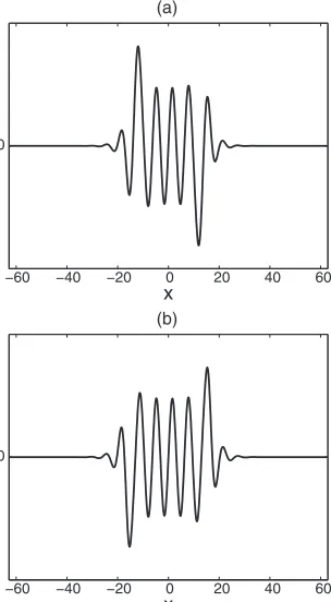
are created in aprimarybifurcation as described in Ref. [25] for a system where like symmetries are destroyed through the imposition of mixed (or Robin) boundary conditions. Depending on the sign ofα, two types of localized solutions may be produced. The localized solutions emerge at the location where forcing is maximum. Thus whenαis positive (negative) the forcing is weakened (strengthened) at the center of the domain and the localized solution emerges from the edge (center) of the domain as shown in Figs.16(c),16(d),17(c), and 17(d) in the upper (lower) subpanels at the bottom. In each case a pair of branches of localized solutions results, in phase and out of phase with the forcing, and each exhibits snaking. When α >0 both the in-phase and out-of-phase solutions exhibit regular snaking [solid lines in Figs. 16(a)

and16(b)]. In contrast, whenα <0 the branches depart at the bottom from the classical picture [dashed lines in Figs.16(a)

−60 −40 −20 0 20 40 60 0

x (a)

−60 −40 −20 0 20 40 60

0

x (b)

FIG. 15. Eigenfunctions at (a) the lower end and (b) the upper end of the S-shaped rung branch shown in Fig.11. Both eigenfunctions are spatially extended indicating that the S-shaped branch is created as a result of the destabilization of theα=0 translation mode.

the snaking diagram theα <0 branch falls rapidly into phase with theα >0 branch. This is, of course, a consequence of the fact that once the structure is broader than a few wavelengths the effect of the heterogeneity is overwhelmed by nucleation of additional oscillations in the homogeneous part of the forcing. The resulting branches do not terminate when the domain is full but instead undergo a prominent overshoot required to accommodate the defect before turning continuously towards larger r and producing large amplitude spatially periodic structures with a defect at the location of the bump. This is so forα >0 as well [Figs.16(a)and16(b)]. Once again the resulting behavior resembles closely that familiar from sys-tems exhibiting localized states with non-Neumann boundary conditions [25,30].

Figures17(a)and17(b)show the corresponding results for SH35, again forα= ±0.5. Except for the doubled frequency of the snaking branches the results resemble qualitatively those in Figs.16(a)and16(b)for SH23. We have not carried out a detailed study of the asymmetric states with the bump heterogeneity. However, in Figs.18and19we show sample bifurcation diagrams showing rung states for SH23 and SH35, respectively. In contrast to Figs. 6 and 10 these connect branches of φ=0 states to themselves, and not to the φ=π states. We believe that this is a consequence of the spatial localization of the forcing function fb. This pushes the φ=0 and φ=π states a distance /2 apart, in contrast to their separationλ/2 when the forcing function isfp (Sec.IIIA).

−0.4 −0.2 0

0 0.2 0.4 0.6 0.8 1

r

N

(a)

−0.4 −0.2 0

0 0.2 0.4 0.6 0.8 1

r

N

(b)

−60 −40 −20 0 20 40 60

(c)

x

−60 −40 −20 0 20 40 60

(d)

x

−1 −0.8 −0.6 −0.4 −0.2 0 0

0.2 0.4 0.6 0.8 1 1.2

r

N

(a)

−1 −0.8 −0.6 −0.4 −0.2 0

0 0.2 0.4 0.6 0.8 1 1.2

r

N

(b)

−60 −40 −20 0 20 40 60

(c)

x

−60 −40 −20 0 20 40 60

(d)

x

FIG. 17. (Color online) (a), (b) Bifurcation diagrams showing N≡ uL2 as a function of r for SH35 with the forcing fb and α= ±0.5. Solution branches with even (resp. odd) parity are shown in (a) [resp. (b)]. Localized branches for positive (negative)αare shown in solid (dashed) lines. (c), (d) Solution profiles at the first five saddle nodes along the snaking branches. The profiles for positive (negative)αare shown in the upper (resp. lower) subpanels. The thin solid line at the bottom of each subpanel indicates the spatial profile of the heterogeneity.

−0.35 −0.32 −0.29 0.2

0.24 0.28

r

N

(a)

−60 −40 −20 0 20 40 60

(b)

x

FIG. 18. (a) Bifurcation diagrams showing N≡ uL2 as a function ofrfor SH23 with the forcingfbandα= −0.5. Dashed line: even parity φ=0 localized states. Dashed-dotted line: asymmetric rung states. (b) A stable asymmetric state with r= −0.307 and N=0.248 on the middle part of the rung [reached in Fig.26(a)]. The bump profile is shown in the lowest panel.

IV. STABILITY

So far we have not discussed the stability properties of the solutions we have found. These are complicated by the presence of the non-neutral translation eigenvalue. This eigenvalue is responsible for the drift of the different steady states with α=0 as soon as the forcing f is turned on, as further discussed in Sec.VII. This drift also selects stationary states from the one-parameter family of such states present whenα=0. It is these “remaining” stationary states that are represented in the bifurcation diagrams of Secs.III AandIII B. The drift velocity can be obtained by an asymptotic calculation when the magnitude of the heterogeneity |α| is small, i.e.,α=α₁ withα₁=O(1) and 1. Introducing the long time scaleT ≡twe write the solution in the form

u(x,t)=u0(x−xc)+ur(x,T), (9)

where u0 is a stable stationary solution obtained for α=0, xc≡xc(T) is the location of a reference point on the solution anduris a correction. Substituting these relations into Eq. (1) we obtain

−0.73 −0.71 −0.69 −0.67 −0.65 −0.63 0.26

0.28 0.3 0.32 0.34

r

N

(a )

−60 −40 −20 0 20 40 60

(b)

x

FIG. 19. (a) Bifurcation diagrams showing N≡ uL2 as a function ofr for SH35 with the forcingfb andα= −0.5. Dashed line: odd parity localized states. Dashed-dotted line: asymmetric rung states. (b) A stable asymmetric state withr= −0.686 andN=0.305 on the middle part of the rung [reached in Fig.26(c)]. The bump profile is shown in the lowest panel.

The contribution of the correction termur can be eliminated by multiplying Eq. (10) byu₀and integrating over the domain, yielding

˙ xc

u₀2 = −rα1f u0u0 +O()= rα1

2

fu2₀ +O().

(11)

Here · · · denotes integration over the domain. From this relation we obtain the drift velocity

dxc dt =

rα 2

fu2

0

u2 0

+O(2). (12)

It follows that stationary solutions correspond to the zeros of fu2

0. There are two types of such solutions, those for which

the maxima of the solution coincide with the maxima of f ( φ=0), and those for which the minima coincide with the maxima off ( φ=π).

We may use these results to determine the stability of these stationary states with respect to the translation mode for |α| 1. We suppose that the stationary solution at t =0 is shifted from its equilibrium position by a small spatial

displacement x. We have

ut(x,0)=∂tu0(x−xc(t))|t₌0+h.o.t.

= −u₀(x− x)rα 2

f(x)u0(x− x)2 u2

0

+h.o.t.

=u₀(x)rα xf

_(x)u

0(x)u0(x)

u2 0

+h.o.t. (13)

To obtain this result we have repeatedly used the fact that at α=0 the quantityfu2

0 =0. From Eq. (13), we now obtain

the eigenvalue of the translation mode,

λ≈ rα 2

f(x)u0(x)2

u₀2 , (14)

indicating that the translation eigenvalue depends linearly on α when |α| 1. We emphasize that the corresponding eigenfunction is a body mode and so is nonzero across the whole structure. This is in contrast with the symmetry-breaking phase modes familiar from theα=0 case which are

wallmodes: for these modes the eigenfunction is nonzero only at the location of the fronts. Of course, when a steady solution loses stability andλbecomes positive the instability does not result in a steadily drifting state; instead the instability creates a pair of steady but asymmetric states towards which the solution evolves [31]. For the body mode the tilt of the resulting asymmetric state is distributed throughout the structure; for a wall mode the asymmetry manifests itself at the location of the fronts only. Examples of such evolution are shown in Sec.VII.

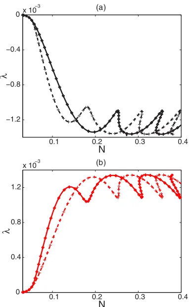
Computations show that for the forcingf =fpthe eigen-valueλ <0 everywhere along the φ=0 branch in SH23, whileλ >0 everywhere along the φ=πbranch (Fig.20), regardless of the sign ofα. Thus the translation mode selects the states along the positive slope segments of the φ=0 branch, cf. Ref. [22], but does not generate any additional bifurcations along the snaking branches. The situation is not nearly so simple for SH35 as discussed next.

0.1 0.2 0.3 0.4 −1.2

−0.8 −0.4

0x 10

−3

N

λ

(a)

0.1 0.2 0.3 0.4

0 0.4 0.8 1.2

x 10−3

N

λ

(b)

FIG. 20. (Color online) The translation eigenvalue of (a) φ=0 and (b) φ=π localized states in SH23 with the forcingfp and δ=1 as a function of N≡ uL2. Solid (dashed) line:α=10−

2

(α= −10−2_{).+: Prediction from Eq. (14).}

homogeneous state; for large structures the instabilities at the front and back are essentially independent, and the ampli-tude and phase modes therefore become degenerate [18,20]. The next two eigenvalues are always negative, emphasizing the fact that the subsequent eigenvalues do not trigger instabilities. The remaining fifth eigenvalue is almost invisible in Fig.22(a)

and is therefore enlarged in Fig.22(b). This eigenvalue is the translation eigenvalue and is nonzero only because α=0. We see that high up the snaking branch this eigenvalue crosses zero at everysecondsaddle node, implying that half of the amplitude-stable segments is drift-stable and half is drift-unstable. This is so for bothα >0 andα <0. Explicit calculation shows that in SH35 the oscillation of the translation mode destabilizes the branch segments connecting the saddle nodes atr2andr3regardless of the sign ofαwhile the segments

connecting r1 and r4 remain stable. This is in contrast to

Ref. [28], where the segmentsr2< r < r3also correspond to

stable even parity states. Figure21shows that for smallαthe analytical prediction (14) of the translation eigenvalue agrees very well with the exact eigenvalue determined numerically. However, for largerαthe exact eigenvalue moves gradually downward, ultimately resulting in the pairwise disappearance of all neutral drift modes. These locations in the parameterα correspond, of course, to the annihilation of the saddle nodes r₂ andr₃ and the disappearance of the associated S-shaped rung branch, as described in Sec.IIIA.

(a)

(b)

0.1 0.2 0.3 0.4

−1 −0.5 0 0.5

1x 10

−5

N

λ

0.1 0.2 0.3 0.4

−1 −0.5 0 0.5

1x 10

−6

N

λ

FIG. 21. (Color online) The translation eigenvalue of (a) even and (b) odd localized states in SH35 with the forcingfpandδ=1 as a function ofN ≡ uL2. Solid (dashed) line:α=10−

4_{(α= −10}−4_).

+: Prediction from Eq. (14).

0.1 0.2 0.3 0.4 −0.8

−0.4 0 0.4 0.8

N

λ

(a)

0.1 0.2 0.3 0.4 −4

−2 0 2

x 10−3

N

λ

(b)

FIG. 22. The linear stability of even localized states in SH35 with the forcingfpandδ=1. (a) The first five leading eigenvalues of the even parity stationary solutions in Fig.9(a)as functions of N≡ uL2, and (b) enlargement of the translation eigenvalue. The thin lines correspond toα=0, while the thick solid (dashed) lines correspond toα=0.03 (α= −0.03).

crossings ofλ=0 in the odd parity case only produce short segments of asymmetric states such as the S-shaped branch shown in Fig.11.

The stability properties of localized states with the forcing fbare similar but not identical. This time we find that in SH23 both φ=0 and φ=π states are stable along the positive slope branch segments whenα >0 while only the φ=0 states are stable along the positive slope branch segments when α <0. The stability of the φ=π states whenα >0 is a consequence of the fact that these states are localized away from the bump and hence inherit the stability properties of the α=0 system. Similarly, both even and odd states of SH35 are stable along the positive slope branches whenα >0, while only the even states are stable along these segments when α <0; the odd states are all unstable.

V. HETEROGENEOUS FORCING ON AO() SPATIAL SCALE

In this section, we present the results when the underlying forcing has a much larger,O(), spatial scale, where we recall is the domain size. The only heterogeneity considered here isfp and we chooseδ=0.05, thereby generating a forcing with a single wavelength in the spatial domain. The forcing

0.1 0.2 0.3

−0.8 −0.4 0 0.4 0.8

N

λ

(a)

0.1 0.2 0.3

−3 −2 −1 0 1 2 3x 10

−3

N

λ

(b)

FIG. 23. (Color online) The linear stability of odd localized states in SH35 with the forcing fp and δ=1. (a) The first five leading eigenvalues of the odd parity stationary solutions in Fig.9(b)

as functions ofN ≡ uL2, and (b) enlargement of the translation (lower curve) and phase (upper curve) eigenvalues whenα=0.03. In (a) the thin lines correspond toα=0, while the thick solid (dashed) lines correspond toα=0.03 (α= −0.03).

resulting from thisfpsatisfies the symmetryR2T/2; as a result

the bifurcation branches forαpositive and negative coincide. The bifurcation diagrams obtained for SH23 and SH35 are qualitatively similar and are shown in Fig.24. The symmetries of the problem are the same as for the bump heterogeneityfb and translation invariance is therefore completely broken. Thus localized structures are again created in a primary bifurcation. These solutions localize rapidly as their norm increases, in the same way as for the bump heterogeneity, and thereafter undergo snaking until the domain is filled. The branches evolve into a large amplitude domain-filling state with further increase in r. However, instead of undergoing snaking in a well-defined interval in r as in the previous section, this time the snaking structure exhibits a prominent slant with a slope that decreases rapidly as|α|increases. Once again the stability of the solutions is similar to that for the caseα=0, with solutions on the positive slope segments stable and the remainder unstable.

−0.6 −0.4 −0.2 0 0

0.2 0.4 0.6 0.8

r

N

(a )

−0.6 −0.4 −0.2 0

0 0.2 0.4 0.6 0.8

r

N

(b )

−1.2 −0.8 −0.4 0

0 0.2 0.4 0.6 0.8 1 1.2

r

N

(c )

−1.2 −0.8 −0.4 0

0 0.2 0.4 0.6 0.8 1 1.2

r

N

(d )

FIG. 24. (Color online) Bifurcation diagrams showing N≡ uL2as a function ofrfor (a), (b) SH23 and (c), (d) SH35 with the forcingfpandδ=0.05. Panels (a) and (c) correspond toα= ±0.1, while (b) and (d) are forα= ±0.5. In (a) and (b) the black [red (or gray)] snaking branch corresponds to solutions withφ=0 (φ=π); in (c) and (d) the black [red (or gray)] lines correspond to even (odd) parity states.

−0.4 −0.2 0.1

0.3 0.5 0.7

a(x

c

)

N

−0.4 −0.2 0.1

0.3 0.5 0.7

a(x

c

)

N

(a)

−0.8 −0.6 0.4

0.6 0.8

a(x

c

)

N

−0.8 −0.6 0.4

0.6 0.8

a(x

c

)

N

(b)

FIG. 25. (Color online) Bifurcation diagrams showing N≡ uL2 from Fig. 24 as a function of ac≡r[1+αcos(xc)], for (a) SH23 and (b) SH35 with the heterogeneityfpandδ=0.05. Left panels correspond toα= ±0.1, while the right panels correspond to α= ±0.5.

snaking interval is almost independent ofα, at least for small |α|, indicating that structures such as that shown in Fig. 24

resembling slanted snaking are indeed the result of a slow variation of theeffectiveforcing parameter, much as in systems with a conserved quantity when these are defined on a periodic domain with a finite period [6,33]. For larger values of|α|the vertical alignment is less good, an observation we attribute to the fact that asN and hencer increases the front profile also changes; as a result the front locationxc, as constructed above, does in fact depend weakly onr, and this dependence is expected to grow with increasing|α|.

VI. SPLITTING OF THE SADDLE NODES

To investigate the splitting of the saddle nodes of the periodic states with φ=0,π as α becomes nonzero, we use the approach of Ref. [29] to calculate the change in the location of the saddle node rsn. We assume that the solutions along a particular branch can be parameterized by a parameters and picks≡ u2

L2 to simplify the calculation. This parametrization is valid at least locally around the saddle nodes. Equation (1) in the stationary case can thus be written as

F[u(x;α,s),r(α,s);α]=0, (15)

where u and r now depend on the parameters α and s. Differentiation ofF with respect toαandsgives

Luα+Frrα+Fα=0, (16)

Lus+Frrs=0, (17)

where

L≡a−(1+∂xx)2+Nu (18)

is a self-adjoint linear operator. Sinceusis the marginal mode at the saddle-node bifurcation,Lusvanishes at the saddle node. Equation (17) shows that this condition translates into the statement thatrs =0 at the saddle node. Multiplying Eq. (16) by 2us and integrating the result over the domain using the fact thatLis self-adjoint, we find that forα=0

2 (usFrrα+ usFα)=rα+rf u2s=0 (19)

at the saddle node. Herev ≡₋/_/2

2v(x)dx. Whenα=0 the

saddle node is located atrsn=r(α,s(α)), where s=s(α) is determined by the conditionrs =0. We haversn =rα+rss andrs=0 at the saddle node. Thus the splitting ofrsnup to O(α) takes the form

rsn(α)=rsn(0)(1−αf u2s)+O(α2). (20)

Relation (20) can be used to explain the observed splitting of the saddle nodes of the periodic branches in the numerical continuation results given in earlier sections. Owing to the nonzero mean of the periodic solutions in SH23, the quantity fpu2is positive (resp. negative) for the periodic branch with φ=0 (resp. φ=π). The solutions grow in amplitude as one passes through the saddle nodes implying thatfpu2s has the same sign asfpu2. The relation (20) now implies that the φ=0 branch hasrsn(α)< rsn(0) while the φ=π branch hasrsn(α)> rsn(0) in agreement with the numerical

results. A similar argument can be used to explain the shift in saddle nodes of the snaking structures observed in SH23 and SH35. The interaction between the forcing and the nucleation of new oscillations at the front and back of the structures which fall into regions of reduced forcing generates the shifts in the saddle nodes observed in Figs.24(a)and24(b).

However, for SH35 with the heterogeneity fp, f u2 vanishes for both even and odd periodic solutions, and the calculation toO(|α|) is insufficient to determine the splitting of the saddle node. A calculation up toO(α2_{) is required. The}

second derivatives ofF with respect toαandsare

Luαα+2(Lα+rαLr)uα+Nuuu2α+Frrrα2

+Frrαα+Fαα+2Frαrα=0, (21)

Luαs+rsLruα+(rαLr+Lα)us+Nuuuαus +Frrrαrs+Frrαs+Fαrrs =0, (22)

Luss+2rsLrus+Nuuus2+Frrrs2+Frrss=0. (23)

From Eq. (1), we see thatFααandFrrare both zero whenα=0. Multiplying Eqs. (21)–(23) by 2us and integrating the result using the fact thatLis self-adjoint, the following relations are obtained at the saddle node whenα=0:

rαα = −2(Nuuuα+2rf −2rf u2s)uαus + 2r(f u2s)2,

(24)

rαs = −2

(Nuuuα+rf −rf u2s)u2s , (25)

rss= −2

u3_sNuu. (26)

The second derivative ofrsntakes the form

r_sn =rαα+2rαss+rss+rss(s)2=rαα− r2

αs rss

, (27)

where we made use ofrs=0 ands= −rαs/rssto obtain the last equality. The splitting toO(α2) therefore takes the form

rsn(α)=rsn(0)(1−αf u2s)

+α2(Nuuuα+rf −rf u2s)u2s 2

u3_sNuu

− (Nuuuα+2rf −2rf u2s)uαus +r(f u2s)2

+O(|α|3). (28)

The factor ofO(α2_{) in Eq. (28) can be determined numerically,}

butuαneeds to be solved for from Eq. (16) before evaluating the integrals. The operatorLhas two marginal modes at the saddle node,usandux, leading to the conditions

uuα =0, uxuα =0. (29)

The first of these ensures theL2_{-norm of the solution is fixed}

saddle nodes with increasing|α|observed in Fig.13can be captured within such a higher order calculation.

For the localized states in SH35fpu2 andfpu2s are both nonzero and the generic results apply. However, their magnitude for the even state is approximately 10 times that for the odd states, thereby explaining the much smaller saddle-node splitting in Fig.9(b)than in Fig.9(a).

VII. PATTERN DYNAMICS IN THE PRESENCE OF HETEROGENEOUS FORCING

The presence of spatially dependent forcing has significant effects on pattern selection. The results in Sec.IVindicate that

−20 −10

0 10

20 0 500

1000

−2 0 2

(a)

x

t u

−20 −10

0 10

20 0 1000

2000 3000

4000 5000

−2 0 2

(b)

x

t u

−20 −10

0 10

20 0 1000

2000 3000

4000 5000

−2 0 2

(c)

x

t u

FIG. 26. Time evolution of (a) an unstable φ=π localized solution in SH23 with forcingfbandα= −0.5, (b) an unstable even localized solution in SH35 with forcingfpwithα=0.1, δ=1, and (c) an unstable odd localized solution in SH35 with forcingfbwith α= −0.5.

in SH23 the φ=πstates that are stable under homogeneous forcing become unstable in the presence of the forcing fp with nonzeroα, regardless of its sign. In contrast, withfbthe φ=π states remain stable when α >0 but lose stability when α <0. In SH35 the odd solutions play a similar role. These can be stable under homogeneous forcing but become unstable in the presence of the forcingfpwith nonzeroαand fbwithα <0. This is also the case for some of the even states in SH35 withfp, for example, those between the saddle nodes atr₂andr₃which become unstable as soon asα=0.

In this section we study the dynamics resulting from these instabilities using direct numerical integration. We use the time-stepping scheme ETD4RK [34] with Fourier basis functions in space. The solutions are dealiased according to the degree of the nonlinearity: half the spectrum is removed for SH23 while two thirds are removed for SH35. The simulations below use 1024 modes.

Whenα=0 time-independent periodic solutions of SH23 have a specific phase relative to the forcingfp, φ=0 (stable) and φ=π(unstable). Initial value simulations starting from a periodic initial condition with φ=0 show that the solution becomes asymmetric as soon as α=0 and starts to drift towards the stable, energetically preferred (with respect toF) state φ=0. This is the case with the forcingfbas well: here the preferred state resembles a periodic structure with a defect in the vicinity of the bump. Localized states also drift as soon as translation invariance is broken. Figure 26(a)shows the evolution of an unstable φ=πstate with the forcingfband α <0: the solution drifts towards a φ=0 state. This state is not stable, however, and the systems finds a stationary but asymmetric state instead [Figs. 18(b)and27]. States of this type are generated from the asymmetric rung states as soon as translation invariance is broken (α=0); Fig.18(b)shows that the dominant peak in the solution is in phase with the imposed bump, but the overall solution is highly asymmetric with respect to this point. We think of solutions of this type as states that would drift in the absence of the bump, but that are trapped or pinned by the bump.

−20 −10 0 10 20 −0.4

−0.3 −0.2 −0.1 0

Δ x

−

∂

F/

∂α

FIG. 27. The quantity −Fα (= 1₂ /2

−/2rfb(x+ x)u0(x)2) in

−40 −20

0 ₀

1 2

3 4

5

x 105

−2 0 2

(a)

x u

t

0 1 2 3 4 5

x 105

−30 −20 −10 0

t

x

(b)

FIG. 28. (a) Time evolution of an unstable φ=0 localized solution in SH23 with fp forcing and α= −0.01, δ=0.05. (b) Location of the maximum of the solution as a function oft. The solid line represents the results of direct numerical simula-tion while the + signs are computed from the asymptotic result in Eq. (12).

For comparison we show in Fig.26(c)the corresponding evolution of an unstable odd state in SH35 with the forcing fb andα <0. The figure shows that the state evolves into a stable stationary but asymmetric state. Figure19(b)shows the resulting final state.

We can use these simulations to compare the observed front speed with the prediction Eq. (12). For this purpose we consider the case of SH23 withfp forcing andα= −0.01 in the same setting as in Sec.V. We pick a stable in-phase localized solution obtained from numerical continuation and shift it horizontally by−10πto generate an initial condition. Figure 28 shows the time evolution and the location of the maximum of the solution as a function of time. The solid line in (b) is obtained by solving the Swift–Hohenberg equation numerically while the data obtained from Eq. (12) is represented using the+symbol. The result shows excellent agreement between the asymptotic calculation and the full numerical result.

VIII. SUMMARY

In this paper we have described the effects of spatial het-erogeneities on the properties of spatially localized structures (LS) in one spatial dimension. For this purpose we have used a modification of the well-studied Swift-Hohenberg equation, focusing on two cases, the quadratic-cubic equation (SH23)

and the cubic-quintic equation (SH35). In each case we applied multiplicative spatial forcing by allowing the parameter a to depend on space. Forcing of this type preserves the homogeneous stateu=0 while selecting preferred locations for the spatial structures, somewhat in the manner of finite domain boundary conditions [25,26]. We first examined the effects of periodic forcing with wavelength equal to the natural wavelength generated by the Swift-Hohenberg equation. This case corresponds therefore to 1:1 spatial resonance, and the behavior observed is characteristic of strong resonance problems. Specifically, we found that LS in phase with the forcing could be stable, while out-of-phase LS were necessarily unstable. In SH23 the former snake in the normal fashion, while the snaking in the latter is incomplete and results in the formation of two-pulse LS, much as in SH23 with mixed boundary conditions [25]. In SH35 even parity states also snake but for small forcing do so between four limiting values; with increased forcing the inner limit points merge via a process resembling that identified in Ref. [28] in connection with the breaking of theu→ −usymmetry of SH35. We have identified an explanation for this behavior and confirmed the predictions by examining the splitting of the saddle nodes as the forcing amplitude α becomes nonzero. In contrast, the odd parity states execute incomplete snaking.

We have also considered the case of an isolated forcing bump on the scale of the natural wavelength of the system and found solutions that are localized at the location of the bump, while others are repelled. We refer to the former as trapped; such states also snake but the snaking branch is now a primary solution branch that evolves, once the domain is full, into an extended defect state, much as occurs in systems with non-Neumann boundary conditions [25]. Finally, we employed periodic forcing with only one period in the (large) domain. Such forcing is locally homogeneous but the effective bifurcation parameter depends on the location. This effect was found to incline the snaking branches present in strictly homogeneous systems, thereby providing an alternative expla-nation of slanted snaking observed in experiments [12,33,35]. Evidently slanted snaking need not arise only as the result of a conserved quantity as in Refs. [6,7,33] but can also be the result of large scale parameter variation across the experimental system.

Throughout we examined the stability of the localized states we have found, identifying both stable and unstable structures as a function of the model parameters. Numerical simulations were performed to identify the longtime fate of unstable solutions. Structures destabilized via an unstable phase mode become asymmetric and undergo drift, a result of the tilting of the effective potential by the heterogeneous forcing, until such time as they become trapped or reach a region characterized by spatially homogeneous parameters.

and optics [39,40], to reaction-diffusion models [41,42] and recent work on models of desertification [43,44]. In addition, localized bump forcing may serve as a model of a persistent perturbation, such as may be applied by a focused optical probe in an optics experiment, in contrast to instantaneous perturbations applied by turning the probe rapidly on and off. The latter example leads to initial value evolution with a different initial condition; the former can lead to persistent

structures trapped by the inhomogeneity whose properties may be tailored by appropriate shaping of the bump profile [45].

ACKNOWLEDGMENTS

We are grateful to D. Avitabile and U. Thiele for helpful discussions. This work was supported by National Science Foundation under the grant DMS-1211953.

[1] K. Ghorayeb and A. Mojtabi,Phys. Fluids9,2339(1997). [2] S. Blanchflower,Phys. Lett. A261,74(1999).

[3] O. Batiste, E. Knobloch, A. Alonso, and I. Mercader,J. Fluid Mech.560,149(2006).

[4] A. Bergeon and E. Knobloch,Phys. Fluids20,034102(2008). [5] I. Mercader, O. Batiste, A. Alonso, and E. Knobloch,J. Fluid

Mech.667,586(2011).

[6] D. Lo Jacono, A. Bergeon, and E. Knobloch,J. Fluid Mech.687,

595(2011).

[7] C. Beaume, A. Bergeon, H.-C. Kao, and E. Knobloch,J. Fluid Mech.717,417(2013).

[8] R. Richter and I. V. Barashenkov,Phys. Rev. Lett.94,184503

(2005).

[9] U. Bortolozzo, M. G. Clerc, and S. Residori,New J. Phys.11,

093037(2009).

[10] T. M. Schneider, J. F. Gibson, and J. Burke,Phys. Rev. Lett.

104,104501(2010).

[11] M. Avila, F. Mellibovsky, N. Roland, and B. Hof,Phys. Rev. Lett.110,224502(2013).

[12] H.-G. Purwins, H. U. B¨odeker, and S. Amiranashvili,Adv. Phys.

59,485(2010).

[13] C. Etrich, U. Peschel, and F. Lederer,Phys. Rev. Lett.79,2454

(1997).

[14] D. V. Skryabin,Phys. Rev. E60,3508(1999).

[15] J. Burke, S. M. Houghton, and E. Knobloch,Phys. Rev. E80,

036202(2009).

[16] J. Burke and E. Knobloch,Chaos17,037102(2007).

[17] A. Alonso, O. Batiste, E. Knobloch, and I. Mercader, in Localized States in Physics: Solitons and Patterns, edited by O. Descalzi, M. G. Clerc, S. Residori, and G. Assanto (Springer, Berlin, 2010), pp. 109–125.

[18] J. Burke and E. Knobloch,Phys. Lett. A360,681(2007). [19] P. D. Woods and A. R. Champneys, Physica D 129, 147

(1999).

[20] M. Beck, J. Knobloch, D. J. B. Lloyd, B. Sandstede, and T. Wagenknecht,SIAM J. Math. Anal.41,936(2009). [21] E. J. Doedel, A. R. Champneys, F. Dercole, T. Fairgrieve,

Y. Kuznetsov, B. Oldeman, R. Paffenroth, B. Sandstede, X. Wang, and C. Zhang,AUTO-07P: Continuation and Bifur-cation Software for Ordinary Differential Equations(Concordia University, Montreal, 2008).

[22] J. Burke and E. Knobloch,Phys. Rev. E73,056211(2006).

[23] A. Bergeon, J. Burke, E. Knobloch, and I. Mercader,Phys. Rev. E78,046201(2008).

[24] D. Lo Jacono, A. Bergeon, and E. Knobloch,Fluid Dyn. Res.

44,031411(2012).

[25] S. M. Houghton and E. Knobloch, Phys. Rev. E80,026210

(2009).

[26] G. Kozyreff, P. Assemat, and S. J. Chapman,Phys. Rev. Lett.

103,164501(2009).

[27] D. Avitabile and H. Schmidt (unpublished).

[28] S. M. Houghton and E. Knobloch, Phys. Rev. E84,016204

(2011).

[29] E. Makrides and B. Sandstede,Physica D268,59(2014). [30] I. Mercader, O. Batiste, A. Alonso, and E. Knobloch,Phys. Rev.

E80,025201(R)(2009).

[31] G. Dangelmayr, J. Hettel, and E. Knobloch,Nonlinearity10,

1093(1997).

[32] P. Hirschberg and E. Knobloch, J. Nonlinear Sci. 7, 537

(1997).

[33] J. H. P. Dawes,SIAM J. Appl. Dyn. Syst.7,186(2008). [34] S. M. Cox and P. C. Matthews,J. Comp. Phys.176,430(2002). [35] W. J. Firth, L. Columbo, and A. J. Scroggie,Phys. Rev. Lett.99,

104503(2007).

[36] R. Manor, A. Hagberg, and E. Meron,Europhys. Lett.83,10005

(2008).

[37] R. Manor, A. Hagberg, and E. Meron,New J. Phys.11,063016

(2009).

[38] E. L. Koschmieder,Adv. Chem. Phys.26,177(1974). [39] S. Barbay, Y. M´enesguen, X. Hachair, L. Leroy, I. Sagnes, and

R. Kuszelewicz,Opt. Lett.31,1504(2006).

[40] P. Parra-Rivas, D. Gomila, M. A. Mat´ıas, and P. Colet,Phys. Rev. Lett.110,064103(2013).

[41] Y. Nishiura, T. Teramoto, X. Yuan, and K.-I. Ueda,Chaos17,

037104(2007).

[42] Y. Nishiura, T. Teramoto, and X. Yuan,Comm. Pure Appl. Anal.

11,307(2012).

[43] M. Tlidi, R. Lefever, and A. Vladimirov, inDissipative Solitons: From Optics to Biology and Medicine, edited by N. Akhmediev and A. Ankiewicz, Lecture Notes in Physics 751 (Springer, New York, 2008), pp. 381–402.

[44] E. Meron,Ecol. Model.234,70(2012).

[45] A. Yochelis, E. Knobloch, Y. Xie, Z. Qu, and A. Garfinkel,