Microscopic basis for pattern formation and anomalous transport in two-dimensional active gels

promoting access to White Rose research papers

White Rose Research Online

Universities of Leeds, Sheffield and York

http://eprints.whiterose.ac.uk/

This is the author’s version of an article published in

Soft Matter

White Rose Research Online URL for this paper:

http://eprints.whiterose.ac.uk/id/eprint/75776

Published article:

Head, DA, Gompper, G and Briels, WJ (2011)

Microscopic basis for pattern

formation and anomalous transport in two-dimensional active gels.

Soft Matter, 7.

3116 - 3126 . ISSN 1744-683X

Microscopic basis for pattern formation and anomalous transport in

two-dimensional active gels

†

David A. Head,

Gerhard Gompper,

and W. J. Briels

Received Xth XXXXXXXXXX 20XX, Accepted Xth XXXXXXXXX 20XX First published on the web Xth XXXXXXXXXX 200X

DOI: 10.1039/b000000x

Active gels are a class of biologically-relevant material containing embedded agents that spontaneously generate forces acting on a sparse filament network. In vitro experiments of protein filaments and molecular motors have revealed a range of non-equilibrium pattern formation resulting from motor motion along filament tracks, and there are a number of hydrodynamic models purporting to describe such systems. Here we present results of extensive simulations designed to elucidate the microscopic basis underpinning macroscopic flow in active gels. Our numerical scheme includes thermal fluctuations in filament positions, excluded volume interactions, and filament elasticity in the form of bending and stretching modes. Motors are represented individually as bipolar springs governed by rate-based rules for attachment, detachment and unidirectional motion of motor heads along the filament contour. We systematically vary motor density and speed, and uncover parameter regions corresponding to unusual statics and dynamics which overlap but do not coincide. The anomalous statics arise at high motor densities and take the form of end-bound localized filament bundles for rapid motors, and extended clusters exhibiting enhanced small-wavenumber density fluctuations and power-law cluster-size distributions for slow, processive motors. Anomalous dynamics arise for slow, processive motors over a range of motor densities, and are most evident as superdiffusive mass transport, which we argue is the consequence of a form of effective self-propulsion resulting from the polar coupling between motors and filaments.

1

Introduction

Living matter fundamentally differs from dead (or passive) media in that it is driven by spontaneously-activating inter-nal processes, depleting some energy reservoir maintained by the organism’s metabolism1–3. This should be contrasted with passive materials which may be driven externally by e.g. an imposed boundary, or simply agitated by thermal noise. An immediate and crucial consequence with regards quanti-tative modeling of living systems is that they do not obey the principles of thermodynamic equilibrium4,5, necessitating the development of novel analytical and theoretical principles if such systems are to be understood on the same level as equi-librium matter. Ideally, such a program should proceed via in-cremental improvements to theory in tandem with experimen-tal verification and guidance, but the enormous complexity of real organisms eliminates facile comparison with any suitably

†Electronic Supplementary Information (ESI) available: [details of any supplementary information available should be included here]. See DOI: 10.1039/b000000x/

a _{Theoretical Soft Matter and Biophysics, Institut f¨ur Festk¨orperforschung,} Forschungszentrum J¨ulich 52425, Germany

b_{Computational Biophysics, University of Twente, 7500 AE Enschede, The} Netherlands

c_{E-mail: [email protected]} d_{E-mail: [email protected]} e_{E-mail: [email protected]}

transparent theory. It is therefore often prudent to treat in vitro systems of known composition and reduced complexity.

This approach has been applied with some success to the

cellular cytoskeleton, a dynamic scaffolding of protein

fila-ments and associated proteins that contributes to the mechan-ical, structural and motility properties of eukaryotic cells1,6–9. This can be classified as an active gel, both because it contains molecular motors that generate

O

and because the filaments themselves can translate or ‘tread-mill’ due to different growth rates at either end. It is possible with reconstituted in vitro active gels to inhibit treadmilling and add permanent biotin-avidin crosslinks between filaments, resulting in a static gel with both thermal and athermal sources of noise, the latter deriving from the action of motor proteins on the network5,10–12_{. These athermal noise sources have been}

shown to violate the fluctuation-dissipation relation5,11_,

cate-gorically placing active gels outside the realm of equilibrium thermodynamics, and the athermal noise spectrum can be re-lated to the properties of motor proteins13–15_.

extends the hydrodynamic equations of liquid crystals in their nematic phase38_{to include active terms (with}

phenomenologi-cal coefficients) obeying the required symmetries20–26_{. These}

active nematodynamic equations admit stable solutions with line defects in the director field, include cylindrical spirals that rotate due to active processes20; these were likened to the vortices seen in quasi-2D microtubule experiments16,17, although no quantitative comparison has yet been made. An alternative approach extends the Smoluchoswki equations for rigid rods39to include active driving27–33, and although these active terms were derived from microscopic considerations, some coarse-graining is still required, resulting in what can be regarded as a mesoscale model.

What is lacking despite this plethora of modelling is a clear picture of the microscopic mechanisms driving the self-organization observed in experiments. Ideally the large-scale equations could be found by coarse-graining a suitable micro-scopic model, but this would inevitably involve approxima-tions whose validity would need to be assessed. Furthermore, the only coarse-graining attempted so far failed to generate all of the terms expected on symmetry grounds, with implications for the formation of vortices31. It is into this state of affairs that simulations can play a key role, permitting as they do full control and access of all microscopic details. Non-Brownian simulations mimicking the microtubule experiments generate asters and apparently vortices16,17,40,41, but did not include ex-cluded volume interactions between filaments and thus lacked nematic elasticity, making comparison to the nematodynamic theories20–26 problematic. Further simplified models with-out filament growth found no defects42_{. Point-like defects}

were also claimed in two-dimensional simulations of inelastic rods43–48_{, but these were somewhat coarse-grained and again}

provided no microscopic picture for the role played by indi-vidual motors.

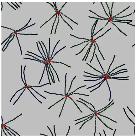
Here we present the results of extensive simulations of a two-dimensional model for active gels, with the goal of com-plementing existing analytical and experimental approaches by providing a microscopic underpinning for any observed non-trivial macroscopic pattern formation. Our chosen numer-ical scheme includes: (i) Mobile motors as the originator of all non-equilibrium effects; (ii) Excluded volume interactions be-tween filaments, so nematic elasticity is present; (iii) Thermal diffusion of filaments, which will be relevant to actin if not microtubule systems; (iv) Mechanical elasticity of filaments, which can store and release elastic energy in the form of bend-ing and stretchbend-ing modes. Filaments are polar, that is they have well-defined[+]and[−]-ends, and motors move strictly towards[+]-ends, breaking microscopic reversibility. Some snapshots are given in Fig. 1. The structures evident in these snapshots, and associated dynamic anomalies, are fully char-acterized below. Given the large aspect ratio of single fila-ments, finite-size effects are pronounced and we have taken

great efforts to control variation with system size for all of the quantities considered.

One of our central findings is that the action of the motors can drive the formation of non-trivial structure formation in one region of parameter space, and anomalous dynamics in a different, albeit overlapping parameter regime. Motor-driven structure formation is most evident for high motor densities, where the nematic ordering breaks down and filament clus-ters form. The nature of these clusclus-ters depends on the motor speed. For motors sufficiently fast to dominate over thermal diffusion, localized clusters form in which the filaments are bound at their[+]-ends, as evident in Fig. 1(b). This can be viewed as non-equilibrium polar ordering on scales compara-ble to the filament length L, that becomes isotropic on much larger lengths. The dynamics of such states is anomalous in that the mean-squared displacement of filament centers ex-hibits a superdiffusive regime in which it scales faster than lin-early in time, but this effect becomes less pronounced as the motor speed increases, a non-intuituve finding that we explain below in terms of a vanishing population of mobile motors.

Maintaining a high motor density but decreasing the motor speed so that motor motion and thermal effects compete, we find a region of parameter space that exhibits both anomalous diffusion and non-trivial structure formation; see Fig. 1(d). Extended, polarised clusters form that can span the system size, generating large voids between the high-density clusters that is evident as an increase, possibly a divergence, of the static structure factor S(q)as the wavenumber q→0. Su-perdiffusive mass transport is most pronounced in this param-eter regime. Nonetheless the polarity of filaments separated by distances comparable to a filament length or more are uncor-related, in contrast to the prevalent assumption of continuum modelling that the polarity field is slowly-varying over such lengths.

This paper is arranged as follows. In Sec. 2 we describe in detail the numerical model, before turning into Sec. 3 to briefly describe the behavior of passive systems in which mo-tors do not move. This provides a comparison for the results of active systems presented in the succeeding section, where we separately focus on static quantities in Sec. 4.1 and then the dynamics in Sec. 4.2. Despite performing a systematic investigation of parameter space, and including the physical mechanisms thought to be necessary for the emergence of the structures seen in the microtubule experiments16,17, we never observe vortices. Possible causes are discussed in Sec. 5.

2

Model

We are interested in determining the universal features of motor-driven filament systems, independent of the atomic de-tails of either the filaments or the motors (or motor clusters). To this end, we describe both filament segments and motors in a simplified manner requiring only a few degrees of freedom, and focus on the collective effects of many motors and fila-ments. See Fig. 2 for a schematic representation of essential aspects of the model, which we now describe in detail.

Filaments are described as polar semi-flexible polymers of monomers with lattice spacing b. Rigidity and contour length are maintained by elastic energies penalizing local fluctuations in both monomer separation and bending. For the former, two monomers instantaneously separated by a distance r incurs a cost δEstretch=πa2E(r−b)2_{/2b, where E is the material’s}

Young’s modulus and a the radius of the cross-section (as-sumed circular)50_{. In addition, the energy for bending by a}

local angleφis given byδEbend=κφ2_{/2b withκthe}

bend-ing modulus, which for a rod with a circular cross-section of radius a is given by κ=πEa4/450. Once thermal fluctua-tions from the solvent are included (see below), and assum-ing sufficient resistance to stretchassum-ing to inhibit contour length fluctuations, this gives a persistence lengthℓp≈κ/2kBT in 2

dimensions. For our parameters,ℓp/L≈10/3 in terms of the

filament length L, so our filaments are semiflexible.

Excluded volume is incorporated as a repulsive potential be-tween non-bonded monomers. We use the repulsive part of the Lennard-Jones potential with rangeσand energyε, truncated and shifted to ensure continuity of the first derivative at the maximum range 21/6σ, i.e. Vev(r) =4ε(σ/r)6

(σ/r)6₋₁ +

ε, with r the distance between monomer centers. To avoid a proliferation of parameters we simply set σ=b, whileε=

5kBT is set sufficiently high to ensure excluded volume

dom-inates over thermal fluctuations for overlapping monomers. Thermal fluctuations arise due to the interaction between the filaments and the solvent. Assuming the usual low-Reynolds number limit for biophysical systems, we adopt a Brownian dynamics algorithm that describes forces due to sol-vent fluctuations in the non-inertial limit51. To better model

(a)

(b)

(c)

(d)

(e)

(f)

the anisotropic friction coefficients for elongated particles39_,

we first project forces parallel and perpendicular to the local filament axis, and then apply the usual displacement incre-ments with solvent friction coefficientsγkandγ⊥=2γk, re-spectively. Note that solvent forces and drag obey the usual fluctuation-dissipation relation via the temperature kBT , so the

solvent is in equilibrium; all non-equilibrium effects derive from the motion of motors, which we now describe.

Motors (or motor clusters) are modeled as two-headed harmonic springs that are simultaneously attached to two monomers; motors with one or no attached heads are not explicitly represented. The spring extension is defined in terms of the separation between the monomer centers relative to its natural length, here taken to be the excluded volume range 21/6_{σ, and the spring stiffness is fixed at k}

BT/b2.

At-tachment, detachment and motor motion are defined by the following rate-based rules. (i) Motors attach at a rate kA

be-tween any two monomers on different filaments whose centers are within a specified distance, which for simplicity we take to be the spring’s natural length 21/6σ. (ii) Both motor heads simultaneously detach at a rate kD that does not depend on

the positions of heads along the filaments, nor on the spring tension, except in that severely stretched motors with elastic energies exceeding≈7.5kBT detach immediately. Increased

detachment rates at filament ends, thought to be important for the formation of vortices (but not asters)17, could easily be in-cluded at a later stage. (iii) Each motor head moves in a Monte Carlo-like manner: The change in motor spring energy∆E for

a head to move m≥1 monomers towards the attached fila-ment’s[+]–end is calculated, and this trial move is accepted with probability kMe−∆E/kBT per unit time if∆E >0, or kM

if∆E<0. Each m is drawn uniformly from the fixed range

[1,mmax], and the acceptance probability is suitably

normal-ized to ensure invariance with respect to mmax. Motors already

in tension are less likely to move due to the increase in strain energy, giving an effective stall force of the order of kBT/b.

Motors already at[+]-ends simply do not move, but may de-tach at the usual rate. Motors do not move if to do so would exceed the maximum spring energy described in (ii).

All filaments have M=30 monomers and hence are of length L=30b, giving an aspect ratio L/b=30. Typically we use a 4L×4L box, but to check for convergence with sys-tem size for any given quantity, we also simulated 6L×6L and 8L×8L boxes for a representative sample of parameter space, corresponding to 2 vertical and 2 horizontal lines in the parameter space discussed below. The area fraction of fila-ments was fixed atφ≈21% throughout, which was checked to give a nematic order parameter close to unity in the absence of motors. At t=0 filaments are placed in a smectic con-figuration to ensure no significant initial overlap, with each filament’s polarity independently chosen to be±ˆp with equal probability. Steady state is identified as when the two–time

Fig. 2 (Color online) Schematic of model parameters. Filament polarity is defined by[+]and[−]-ends as denoted in the figure. Motors are 2-headed springs defined by attach, detach and motion rates kA, kDand kM, respectively, where the movement rate is attenuated by an exponential factor depending on the increase in spring energy∆E for the proposed move (∆E=0 if this change is negative). See text for details.

mean squared displacement of filament centres–of–mass x(t), h∆r2(tw,tw+t)i=h|x(tw+t)−x(tw)|2i, ceases to depend on twand only varies with the lag time t, i.e. becomesh∆r2(t)i.

The results from the simulations will be described in terms of the two dimensionless parameters kA/kDand kMτb, where τb=Lbγ/4kBT is the time for an isolated filament’s centre–

of–mass to translationally diffuse over one monomer diam-eter. Thus kA/kD gives a rough measure of motor

den-sity, and kMτbmeasures the competing effects of motor

mo-tion to thermal diffusion over lengths of the monomer spac-ing b. We fix the value of kD to be small relative to τ−_b1, i.e. kDτb=7.5×10−3≪1, and consider kM varying from kM≪kDto kM≫kD, where the former case corresponds to

non-processive motors that detach before significant motion, and the latter to processive motors which may move many monomers before detaching.

3

Passive systems: k

≡

0

We first summarize the behavior of passive systems with

kM=0, before turning to active systems with kM>0.

With-out motor motion, filament polarity is irrelevant and the time-averaged effect of motor attachment and detachment is to generate an effective attraction between filaments. As the ratio kA/kD between attachment and detachment rates

in-creases, the magnitude of motor-mediated attraction increases and induce a heterogeneous density distribution as evident in Fig. 1(f). Increasing kA/kDeven further gives a percolating

network that nonetheless does not fully phase separate over our simulation time.

To identify the length scales associated with the den-sity fluctuations, we calculate the static structure factor

S(q) of filament centers, defined as the angular average of S(q) =N−1h|n(q)|2_{i over ˆq=q/q with q=|q|. Here,} n(q) =∑N

α=1e−iq·x α

0.2 0.5 1 2 5

q / [2 /L]

10-1 100 101

S(

q)

kA/kD=80

kA/kD=60

kA/kD=40

kA/kD=20

kA/kD=5

kA/kD=1

Fig. 3 (Color online) Static structure factor S(q)for kM=0 and the kA/kDgiven in the key on log-log axes. The horizontal and vertical dotted lines correspond to S(q) =1 and q=2π/L, respectively, with L the filament length. Error bars give the spread between

independent runs. In all cases the system size was 6L×6L.

1≤kA/kD≤80 are shown in Fig. 3. For low kA/kD, S(q)

exhibits a small peak around the wavenumber corresponding to the filament length L, suggesting a slight degree of smectic ordering with filaments aligned end-to-end, before decaying quadratically for smaller q. Increasing kA/kDto around 40,

corresponding to

O

en-hances the height of this peak. Snapshots such as Fig. 1(f) reveal local filament bundles that align end-to-end, explaining this peak. For kA/kDin the range 60—80, the S(q)collapse

onto a single curve with S(q)≈1−3 as q→0 and snapshots reveal similar pictures of percolating networks. It is clear that the system does not phase separate for kA/kD≥60 on our

simulation times, but instead undergoes kinetic arrest into a long-lived metastable gel. We therefore restrict attention to

kA/kD≤40 for the active systems in Sec. 4.

One of our key findings for active systems is the existence of enhanced diffusion, so for comparison we present in Fig. 4 the mean-squared displacements for passive systems. Given the lack of motor-mediated driving, the sole effect of motors is to bind filaments and thus reduce self-diffusion, and this trend is immediately apparent from the figure. For low mo-tor densities the mass transport is roughly diffusive, with a diffusion constant that decreases with increasing kA/kD and

the binding between filaments increases. At high attach rates the mass transport is substantially reduced, and never becomes fully diffusive over our data window, instead giving weak sub-diffusionh∆r2i ∼tαwithα≈0.9 at the maximum time lags available. We nonetheless expect normal diffusion withα=1 to be recovered at late times.

102 ₁₀3

t/

b 10-3

10-2 10-1 100

r

2

/L

2

kA/kD=1

kA/kD=5

kA/kD=20

kA/kD=40

kA/kD=60

kA/kD=80

Fig. 4 (Color online) Mean squared displacementh∆r2ifor kM=0 and kA/kDgiven in the key for the same systems as Fig. 3. The thick dashed line has slope 1 corresponding to normal diffusive scaling

h∆r2i∝t, and the solid horizontal line corresponds to displacements

equal to the filament length.

4

Active systems: k

>

0

The movement of motor heads along the polar filaments gen-erates equal-and-opposite forces that drive relative motion be-tween filaments or filament clusters. Non-trivial flows and pattern formation may thus become stable. In this section we describe the structure and dynamics of active systems in terms of the 2 dimensionless parameters kA/kD, which broadly

corresponds to the density of motors, and the bare motor speed kMτb.

4.1 Statics

Snapshots for systems with mobile motors reveal similar fila-ment ordering as for static motors when kA/kDremains below

some crossover value. This crossover value depends on pa-rameters such as filament length and motor spring stiffness, and for the systems considered here occurs around kA/kD≈

15. When kA/kDexceeds this value, the increased motor

den-sity induces filaments clustering and non-trivial structure for-mation, the nature of which depends on the speed of the mo-tors. For kM≪kD, motors detach at a faster rate than moving

and become non-processive. Filaments form apolar bundles similar to the passive case kM≡0. Conversely, for kMτb≫1

motor motion dominates over thermal diffusion and we ob-serve filament clusters bound at their[+]-ends as in Fig. 1(b). For the intermediate regime kDτb≪kMτb≪1, motors are

processive but compete with diffusion in structure formation. This results in the extended clusters evident in Fig. 1(d).

in-100 101

kA/kD

10-2 10-1 100 101

n mot

/

N

kMb=0

kMb=7.510

2

kMb=7.510

1

kMb=7.5

kMb=75

Fig. 5 (Color online) Number of motors per filament nM/N versus kA/kDfor the dimensionless motor rates kMτbgiven in the key. The thick black line segment has slope 1. For all lines, symbols are larger than the error bars.

creased. As plotted in Fig. 5, the number of motors per filament is roughly proportional to kA/kD, with a prefactor

that decreases with motor speed kM. This linear dependency

on kA/kD can be understood as the steady state solution of

the simple rate equation∂tnmot∝kA−nmotkD governing the

number nmotof attached motors between two monomers held

within the proscribed attachment range. Deviations from strict linearity are evident at high kA/kD>

O

in-duce clustering and the global attachment rate becomes cou-pled to structure formation. The decrease in motor density for high kMis likely due to the greater fraction of motors stretched

close to the detachment limit mentioned in Sec. 2, but this ef-fect is reduced for higher kA/kD when the densities become

similar for all motor speeds.

4.1.1 Cluster size distributions: To quantify the cluster-ing apparent in snapshots, we first consider the distribution

P(nc) of clusters consisting of nc filaments, averaged over

time and independent runs, where two filaments are consid-ered to belong to the same cluster if there is at least one mo-tor simultaneously attached to both. The mean cluster size hnci=∑ncncP(nc)is plotted in Fig. 6, and reveals a

mono-tonic increase with kA/kDfollowing a roughly exponential

re-lationship. It also decreases with increasing motor speed kM,

in part because the density of motors decreases (see Fig. 5), and also because they drive the formation of localised fila-ment clusters bound at their ends. Increasing the system size increases cluster sizes for high kA/kD, but the effect is small

on logarithmic scales.

Considering only the mean cluster sizehnci obscures the

fact that the shape of the full distribution P(nc)qualitatively

0 5 10 15 20 25 30 35 40

kA/kD

100 101 102

nc

kMb=0

kM

b=7.510 2

kMb=7.510

1

kM

b=7.5

kMb=75

Fig. 6 (Color online) Mean number of filaments in a clusterhnci versus kA/kDfor the motor speeds given in the key. The system size was fixed at 4L×4L and error bars are smaller than the symbols.

changes as the parameter space is traversed, see Fig. 7. For most of the parameter space considered, P(nc)is well approx-imated by a simple exponential decay, and does not vary with system size. However, for high kA/kDand kMτb<∼1, the

dis-tribution P(nc) deviates from an exponential, in two ways.

Firstly, a second peak corresponding to system-spanning clus-ters with nc≈N emerges for kMτb<∼1. Secondly, and only

for slow, processive motors with kDτb<∼kMτb<∼1, the small-nc

decay becomes power law rather than exponential. Although noisy, this algebraic decay can be approximately fitted by an exponent -2, as shown in Fig. 7. We note that the region of pa-rameter space for which P(nc)exhibits power-law decay

co-incides with those parameters that exhibit anomalous small-wavenumber density fluctuations, as described in Sec. 4.1.2.

The magnitude of the second peak decays monotonically with increasing system size, suggesting it will vanish in the limit of large system size. This is apparent in plots of the inte-grated area of the second peak, P(nc≥N/2) =∑_nN_c=N/2P(nc),

which can be understood as the probability to find a cluster that is comparable in extent to the system size. The lower cut-off N/2 is arbitrary, but as long as it falls into the middle region where P(nc)≈0, as here, its precise choice does not

measurably alter the result. As shown in the inset to Fig. 7, this quantity decays roughly as N−1. P(nc≥N/2)also

mono-tonically decreases with increasing kMτbas show in the figure,

before vanishing entirely when kMτb>

O

4.1.2 Small-wave number density fluctuations: Al-though useful for considering connectivity, the cluster distri-bution P(nc)gives no information regarding spatial

100 101 102

nc

10-7 10-6 10-5 10-4 10-3 10-2 10-1

P(

nc

)

P(ncN/2)

N

8L8L

6L6L

4L4L

200 400 600

0.2 0.4 0.6 0.8

1

Fig. 7 (Color online) Log-log plot of the distribution P(nc)of cluster sizes ncfor kA/kD=40, kMτb=0.075 and the system sizes given in the key. The thick, dashed diagonal line has a slope of−2, and the vertical lines correspond to nc=N with N=175, 400 and 711 the total number of filaments in the system. (Inset) P(nc≥N/2) versus N on log-log axes for (from top to bottom) kMτb=0, 7.5×10−3, 7.5×10−2and 7.5×10−1. P(nc≥N/2)≡0 for higher kMτb. The thick black line segment has a slope of−1.

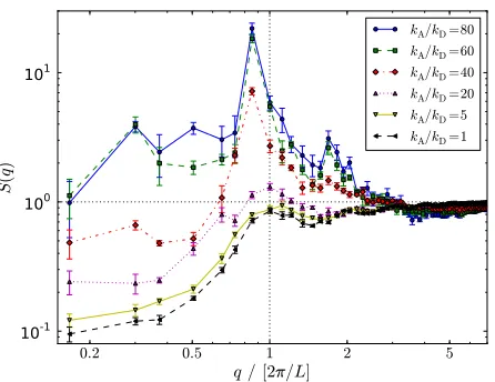
the distribution of mass centers it is useful to look at the static structure factor S(q)as defined in Sec. 3. Fig. 8 shows the vari-ation of S(q)with kMτbfor fixed kA/kD=40. Focussing on

the S(q→0)behavior reveals a non-monotonic dependence on motor speed: for fast motors kMτb>

O

non-processive motors kM<kD, S(q)decays to some small value

as q→0. For intermediate kM, S(q)increases, possibly

di-vergently, with decreasing q, which coincides with the void formation evident in snapshots.

The limited number of data points and poor statistics for small q makes it difficult to characterize the behavior of S(q)

in this limit. Nonetheless some semi-quantitative observa-tions can be made by fitting each S(q)to the form A+Bqc+

Ce−(q/[2π/L]−1)2/D2 over the range q≤2qL, which provides a

stable fit for all parameters considered. Although the fitted exponent c is somewhat susceptible to finite size effects, we consistently observe values close to c=2 for low motor den-sities kA/kD≈1, or very slow or fast motors, kM≪kD and kMτb≫1 respectively. For high kA/kDand intermediate kMτb, c decreases and becomes negative. Although the magnitude of

the fitted exponent depends strongly on system size, the sign does not, suggesting some form of small-wavenumber struc-ture will persist for large system size.

A divergent S(q)was predicted from hydrodynamic equa-tions of active nematic systems with an exponent c=−252_,

and was interpreted as emergent directed motion deriving from the coupling of elastic modes with the breaking of

time-0.2 0.5 1 2 3

q / [2/L]

0.25 0.5 1 2 5 10

S(

q)

kMb=0

kMb=7.510

3

kMb=7.510

2

kMb=7.510

1

kMb=7.5

Fig. 8 (Color online) Static structure factor S(q)for kA/kD=40 and the motor speeds given in the key, for system sizes 8L×8L. For clarity only error bars for kMτb=0.075 are shown; others are comparable. The horizontal and vertical dotted lines corresponds to

S(q) =1 and q=2π/L respectively.

reversal invariance in driven states3. We shall later argue for a form of emergent directed motion in our system when dis-cussing the dynamics in Sec. 4.2, which derives however from the polar coupling between motors and filaments. It is possi-ble that emergent directed motion drives the small wavenum-ber density fluctuations in both systems. As described in Sec. 4.2.1, the parameter values for which exponents c<0 arise coincide with those for which superdiffusive mass trans-port is most pronounced. It is interesting to note that a causal link between superdiffusion and small wavenumber fluctua-tions has been hypothesized from systems lacking orienta-tional degrees of freedom53, in broad agreement with our find-ings.

4.1.3 Nematic and polar ordering: We now move be-yond density fluctuations and consider the orientational de-grees of freedom. Let ˆpαdenote the unit polarity vector from the [−]-end to the [+]-end for each of the N filaments α=

1. . .N. From this can be defined the traceless nematic order

tensor Qα_{i j}=pˆα_ipˆα_j−1

2δi j. The two-dimensional nematic order

parameter S2Dis then defined by(S2D)2=2

hQi ji

2

, where hQi ji=N−1∑αQαi j andk. . .k

2 _{denotes the Euclidean norm}

Ai j

=∑i_,jA2_{i j}. S2D varies from 0 to 1, with 1 for perfect

nematic ordering and 0 when there is no net preferred orienta-tion, such as for an isotropic state, asters etc. A contour plot of

S2Dfor kA/kDand kMτbis given in Fig. 9, and confirms what

is visible from snapshots in Fig. 1, namely that nematic order-ing breaks down for kA/kD>∼15 and processive motors with kM≫kD. This data is for the smallest system size, for which

checked and confirms the crossover to low S2Dis robust. The

value of S2Dmay be approaching zero for points in the upper

right of this plot, but the poor statistics and limited number of points rules out extrapolation to the infinite system-size limit. The nematic order parameter S2Dtell us nothing about

cor-relations in the polarity of filaments. To consider correla-tions in filament polarity, we must go beyond this nematic de-scription and consider order parameters that respect reverses in polarity ˆp→ −ˆp. Firstly we note that the mean polarity hˆpi=N−1_∑

αˆpαvanishes for the entire parameter space con-sidered here. This is in agreement with the theoretical predic-tion that states with non-zero mean filament polarity are only stable if the motors are polar, i.e. have attachment rates that depends on the relative filament polarity32, unlike the apolar motors considered here for which the attachment rate depends only on separation.

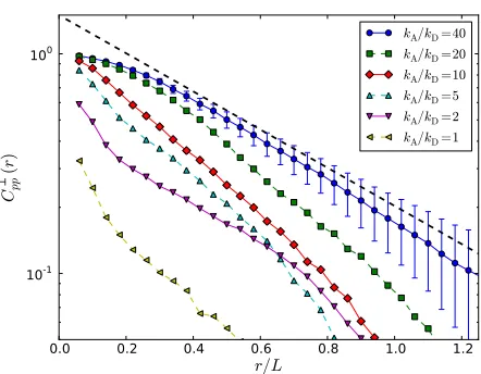
It is natural to consider spatial correlations in polarity along directions parallel to the filament axis separately to those in perpendicular directions. We therefore define the perpendicu-lar poperpendicu-larity correlation function C⊥_pp(r)as

C⊥_pp(r) = ∑α,βˆp

α_·ˆpβ_{δ(r− |x}α_−xβ_|)sin2_θ ∑α,βδ(r− |xα−xβ|)sin2θ

(1)

whereθis the angle between ˆpαand xβ−xα( ˆpβcould equally have been chosen due to the symmetry of Eq. (1)). The corre-sponding parallel function Ckpp(r)is defined analogously, with

the sin2θ weighting factors replaced by cos2θ_{. Both}

pro-jections exhibit approximate exponential decay with r, with longer-range correlations for higher motor densities kA/kD, as

demonstrated in Fig. 10. These correlations become shorter range as kM→0, confirming the smooth approach to the

pas-sive limit kM=0 when all polarity correlations trivially

van-ish. It should be noted that significant polarity correlations are not mutually exclusive with nematic ordering. With regards to finite-size effects, the data shows no apparent trend with system size for all of the parameter space except for the high

kA/kDand kDτb<∼kMτb<∼1 when extended polar clusters arise, for which the range of polarity correlations was still increas-ing for the largest system sizes simulated. Finally, we never observe significant correlations on lengths larger than the fila-ment length L, which will be discussed in Sec. 5 in relation to hydrodynamic modelling.

4.2 Dynamics

Motor motion represents an energy flux driving relative fila-ment motion in violation of the principles of thermodynamic equilibrium, and might therefore be expected to result in anomalous transport properties. Data confirming this

expec-1 2 5 10 20 40

kA/kD

103

102

101

1 10

kM

b

kDb

0.0 0.2 0.4 0.6 0.8 1.0

Fig. 9 (Color online) Nematic ordering parameter S2Dfor kA/kD and kMτbfor fixed system size 4L×4L. In this figure, and in Fig. 12 below, the white discs denote actual data points; linear interpolation within the enclosing triangle is used between points. The thick horizontal dashed white line corresponds to kM=kD.

0.0 0.2 0.4 0.6 0.8 1.0 1.2

r/L

10-1

100

C

pp

(r

)

kA/kD=40

kA/kD=20

kA/kD=10

kA/kD=5

kA/kD=2

kA/kD=1

Fig. 10 (Color online) The transverse polarity correlation function

Fig. 11 (Color online) Emergence of directional motion on the one-filament level under the action of motors, denoted by the short horizontal lines. (a) Net zero displacement for parallel filaments. (b) Net displacement towards the[−]–end for both filaments in an anti–parallel pairing.

tation is provided in this section. The key observation under-lying these findings is that the coupling between motors and filaments is polar, in that motor heads move strictly towards filament[+]-ends. Filaments are thus expected to move in the direction of their[−]-ends in response to the motor forces, as seen by considering connected parallel and anti-parallel fila-ment pairs as in Fig. 11. This effect also emerges from one-dimensional continuum modeling54,55. Thus filaments may move persistently in a direction that is coupled with their po-larity. This scenario is reminiscent of self-propelled parti-cles that are known to typically exhibit enhanced mass diffu-sion, such as an anomalous scaling with time of displacements transverse to particle motion56–58 _{or a longitudinal diffusion}

constant increased by the activity59_{. In this light, anomalous}

transport should also be expected here.

To confirm the correlations between filament motion and polarity, the filament velocity must be defined, for which it is necessary to average over a finite time interval since there is no instantaneous velocity in Brownian dynamics. We de-fine the velocity of filamentα at time t to be vα= [xα(t+

∆t)−xα(t)]/∆t where∆t ≈65τb, corresponding to trajecto-ries spanning a few monomer diameters. Correlations between polarity and velocity are then easily quantified as hv·ˆpi/v

with v=phv·vithe mean filament speed. This is plotted in Fig. 12, and shows higher correlations for large kA/kD

and kMτb∼10−2−10−1, which we will show below is also

roughly where the degree of anomalous mass transport is high-est. Note also that the correlations are negative, confirming filaments move in the direction of their[−]-ends.

1 2 5 10 20 40

kA/kD 103

102 101 1 10

kM

b

kD

b

-0.40 -0.35 -0.30 -0.25 -0.20 -0.15 -0.10 -0.05 0.00

Fig. 12 (Color online) Correlation between individual filament velocity and its polarity,hv·pˆi/v, versus kA/kDand kMτb. As this quantity is relatively insensitive to system size, the largest available system was selected for each point.

4.2.1 Super-diffusive mass transport: Mass transport is conveniently quantified by the mean squared displacements of filament centers,h∆r2(t)i, where for simplicity we average over filament polarity. For the available time window, which typically corresponds to displacements from a fraction of b to a few L, a slow, diffusive or sub-diffusive region is ob-served at small times, sometimes followed by a crossover to super-diffusive scaling at later times in whichh∆r2(t)i ∼tα

withα>1. See Fig. 13 for some examples. The variation of these curves with system size is weak or non-existent. As with the passive case in Sec. 3, we presume an eventual crossover to normal diffusion withα=1 for lag times exceeding our achievable time window.

To quantify the extent of deviation from normal diffusion as a function of the microscopic parameters, it is convenient to condense the variation of logarithmic slopeαover the data window into a single scalar. To do this, we first smooth the data by fitting each curve to the sum of two power laws, h∆r2_i=C

1tc1+C2tc2, which gives a reasonable fit in all

cases. We then take the logarithmic slope of this fit at the point when h∆r2_i=L2_{. The result is given in Fig. 14, and}

shows a decrease in anomalous diffusion away from the peak value at high kA/kD and motor speeds roughly in the range kDτb<∼kMτb<∼1. Choosing a different point along the curve to

extract the slope results in different values but similar trends. A striking feature of Fig. 14 is the non-monotonicity of the degree of anomalous diffusion with motor speed kM, which

approaches normal diffusion for kMτb≫1. The reason is not

101 ₁₀2 ₁₀3

t/b

210

4

510

4

103

210

3

r

2/t

!

(

"

b

/L

2)

# $r

2% =L2 #

$r 2%

&t

kA/kD=1

kA/kD=5

kA/kD=20

kA/kD=40

Fig. 13 (Color online) Mean squared displacements divided by time,h∆r2_{i/t, so that normal diffusive scalingh∆r}2_{i∝t shows up as} a horizontal line. Here kMτb=0.075, the system size was 8L×8L and the kA/kDare given in the legend. The thick dashed lines are fits to C1tc1+C2tc2for each set of data points. The black horizontal line is to guide the eye, whereas the diagonal black line corresponds (on these axes) toh∆r2i=L2and confirms trajectories exceed the filament length for these data sets.

[+]-end where they then stall. Indeed, the fraction of motors with at least one head attached to a [+]-end never drops be-low 80% for kMτb≥1. Since such heads can no longer move,

they do not drive filament separation and the net motor activity decreases, restoring normal diffusion.

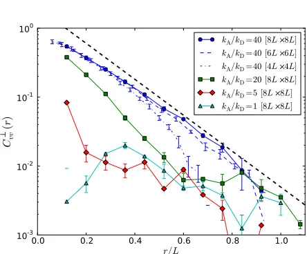
4.2.2 Velocity correlations: Using the same definition of filament velocity vαas above, it is possible to calculate spatial correlations in velocities projected parallel Cvvk(r)and

perpen-dicular C_vv⊥(r)to the filament axis. Here, Cvvk,⊥(r)are defined

analogously to the polarity correlations in Eq. (1), except with the ˆpα replaced by vα/v with v the mean filament speed as

before. Examples are given in Fig. 15, demonstrating a grow-ing range of correlated motion as the motor density increases. This trend was observed throughout the parameter space con-sidered.

Also shown Fig. 15 is an example of the variation with sys-tem size for the highest kA/kD, which demonstrates

conver-gence for the two largest system sizes considered. The decay is exponential, approximately of the form e−r/[L/6] and thus becomes negligibly small on lengths on the order of the fil-ament length L. We never observe correlations decaying on lengths larger than L, and conclude velocities on lengths much larger than the filament length are uncorrelated, a point that is discussed in Sec. 5.

10-4 ₁₀-3 ₁₀-2 ₁₀-1 ₁₀0 ₁₀1 ₁₀2

kM'b

1.0 1.1 1.2 1.3 1.4 1.5 1.6

(

kA/kD=40

kA/kD=20

k_A/k_D=5

kA/kD=1

Fig. 14 (Color online) Scaling of the mean squared displacement with time t, i.e.α=∂lnh∆r2_{(t)i/∂lnt, at the point when}

h∆r2i=L2, versus kMτbfor the kA/kDgiven in the key. For clarity only error bars for kA/kD=20 are shown; others are comparable

0.0 0.2 0.4 0.6 0.8 1.0

r/L

10-3

10-2

10-1

100

C

) vv

(r

)

kA/kD=40 [8L*8L]

kA/kD=40 [6L*6L]

kA/kD=40 [4L*4L]

k_A/k_D=20 [8L*8L]

kA/kD=5 [8L*8L]

kA/kD=1 [8L*8L]

Fig. 16 (Color online) Example of asters at low density with area fractionφ≈5.3%. The system parameters were kA/kD=250, kMτb=75. Motors are short straight lines concentrated at filament [+]-ends.

5

Discussion

It is apparent from the results described above that for the con-sidered density of φ≈21%, structures similar to the asters and vortices in the microtubule experiments16,17 are never re-produced. The absence of asters may be a simple matter of density. The end-bound clusters formed by rapid motors in Fig. 1(b) are not able to form circular structures due to steric hinderance with nearby clusters. Lowering the filament den-sity removes this effect, permitting full asters consisting of a single layer of filaments to form, as demonstrated in Fig. 16. However, vortices did not arise at lower densities, even when increased motor detachment rates at[+]-ends was included. We note that a continuum model37 _{that extended an earlier}

version35_{to include, amongst other features, a form of steric}

hinderance between filaments, favored asters over vortices rel-ative to the earlier work, suggesting excluded volume may also be a factor. Here, we expand upon the relationship between our numerical findings and the related theory and experiments that has already been touched upon, with an emphasis on pos-sible reasons for the non-observation of vortices.

5.1 Comparison to experiments

In their in vitro actin-myosin experiments, Backouche et al. claimed that active structure formation was only possible with the addition of a small concentration of the passive crosslinker

fascin19_{. A small fraction of passive crosslinks between}

adja-cent filaments has also been predicted to significantly increase their rate of alignment by mobile motors48_{. Since no passive}

crosslinkers were included in our simulation, this might be a factor in the qualitatively different structures found here. Fur-thermore, fascin is a bundling protein that promotes the forma-tion of polar actin bundles64,65, thus its dominant role may in fact be to permit non-zero mean polarity. If so, it may play the role of the polar motor clusters that preferentially bind to par-allel (as opposed to anti-parpar-allel) filaments, which were shown theoretically to stabilize homogenous polarized states and pro-duce a correspondingly richer stability diagram32. However, there is no reason to suppose that polarity-dependent binding of active or passive components played a role in the micro-tubule experiments, and was not included in the associated simulations16,17_{, suggesting this is not a reason for the}

non-emergence of vortices in our work.

Apart from molecular motors, a second form of non-equilibrium activity in biofilament gels is the spontaneous translation of filament center-of-mass via unequal monomer addition rates at opposite ends, known as treadmilling and prevalent in vivo9. If present, this would place the system into the class of self-propelled particles, for which a richer variety of structure and dynamics is expected3,56–59,66,67. However, treadmilling was thought not to play a role in the actin-myosin experiments19, and was inhibited to some extent by taxol in the microtubule experiments (although microtubule growth

was present)16,17. Until the role of treadmilling or filament growth is categorically denied experimentally this remains a possible missing factor, but without further experimental guid-ance we can merely speculate on its possible role. Including such features numerically should be straightforward, and in-deed has already been performed for simulations of branching networks68–70.

5.2 Comparison to hydrodynamic models

An assumption common to many of the analytical models is that the velocity and polarity fields are hydrodynamic, in the sense that they have long-wavelength components extending across lengths much larger than the filament length L. In con-trast, as described in Secs. 4.1 and 4.2 above, we never ob-serve polarity or velocity correlations that decay on lengths larger than L. It is possible that long-wavelength correlations emerge at much higher filament densities, but we were not able to check this so far due to computational limitations. Al-ternatively, our numerical scheme may be oversimplified, in that momentum is not conserved by the solvent-filament in-teractions. Since the standard argument for the emergence of a hydrodynamic velocity field requires momentum conserva-tion71_{, this may explain its absence, but correcting for this}

omission numerically is difficult and will require ad hoc mod-ification of the driving terms such as in Ref.72, or the incorpo-ration of full hydrodynamic interactions73.

A slowly varying polarity field is assumed in all theoretical models and coarse-graining schemes20–37_{. The short-ranged}

decay of the polarity correlations in our simulations therefore makes the comparison of the results difficult. This may be partly a question of time scale. For the density considered here, the rotational diffusion time for filaments to significantly change orientation can be large. This is particularly true when the nematic order parameter S2Dis close to unity, when the

orientation autocorrelation function decays by as little as 5% over a production run. This may inhibit the formation of large, polarity-correlated regions. Nonetheless even in this region of parameter space, motor-driven translational separation of fil-aments according to their polarity does occur. Furthermore when S2D≪1, filament rotation is substantially enhanced.

The lack of long-wavelength polarity correlations is therefore somewhat of a mystery.

The nematodynamic theories take as an input parameter the active stress generated on filaments, whose sign deter-mines if this stress is contractile or extensile20,23. Our micro-scopic approach does not impose the sign of the force dipoles generated by motors, so instead it must be measured. The mean dipole moment acting between filament pairs is defined as κ= _N1

(αβ)∑(αβ)F

αβ_·(xβ_−xα_{), where the sum is over all} N_(αβ) filaments pairs (α,β) connected by at least one mo-tor, and Fαβ is the total force onα due to motors connect-ingαandβ. Thusκ>0 corresponds to contractile dipoles, andκ<0 to extensile ones. Preliminary results are given in Fig. 17, demonstrating uniformly contractile stressκ>0 with a magnitude that reaches a maximum for intermediate motor speeds kDτb<kMτb<1. An alternative measure in which

both Fαβand xβ−xαare first projected along the filaments’ axes before summing, as defined in the figure caption, fol-lows the same trend. Thus our motor rules lead to contractile

10-4 ₁₀-3 ₁₀-2 ₁₀-1 ₁₀0 ₁₀1

kM+b 0

5 10 15 20

,

/kB

T

Normal Projected

Fig. 17 (Color online) Variation of the dipole moment with kMfor kA/kD=40 and system size 4L×4L in steady state. The upper line gives the mean dipole momentκ= 1

N(αβ)∑(αβ)F

αβ_·(xβ_−xα_)as

defined in the text, and the lower line gives the projected equivalent κproj₌ 1

2N(αβ)∑(αβ) n

(Fαβ·pˆα)(∆xαβ·ˆpα) + (Fβα·ˆpβ)(∆xβα·ˆpβ)o with ˆpα, ˆpβthe polarity unit vectors for filamentsαandβresp.

active stresses, theoretically predicted to give the richest be-haviour20,23. There is also a slight but measurable reduction of≈0.4% in the mean filament contour length whenκis at its highest, confirming contractility.

Acknowledgements

The authors would like to thank J. Padding, I G¨otze and J. El-geti for useful discussions. Financial support of this project by the European Network of Excellence “SoftComp” though a joint postdoctoral fellowship for DAH is gratefully acknowl-edged.

References

1 B. Alberts, D. Bray, J. Lewis, M. Raff , K. Roberts and J. D. Watson, Molecular Biology of the Cell (Garland, New York, 1994).

2 T. B. Liverpool, Phil. Trans. Roy. Soc. A 364, 3335 (2006). 3 S. Ramaswamy, Ann. Rev. Cond. Matt. Phys. 1, 323 (2010). 4 A. W. C. Lau, B. D. Hoffman, A. Davies, J. C. Crocker, and

T. C. Lubensky, Phys. Rev. Lett. 91, 198101 (2003). 5 D. Mizuno, C. Tardin, C. F. Schmidt and F. C. MacKintosh,

Science 315, 370 (2007).

7 A. B. Kolomeisky and M. E. Fisher, Annu. Rev. Phys. Chem. 58, 675 (2007).

8 Mechanics of the Cell, D. Boal (CUP, Cambridge, 2002). 9 Cell movements: From Molecules to Motility, D. Bray

(Gar-land, New York, 2001).

10 D. P. Kiehart and R. Feghali, J. Cell. Biol. 103, 1517 (1986).

11 D. Mizuno, D. A. Head, F. C. MacKintosh and C. F. Schmidt, Macromolecules 41, 7194 (2008).

12 D. Mizuno, R. Bacabac, C. Tardin, D. A. Head and C. F. Schmidt, Phys. Rev. Lett. 102, 168102 (2009).

13 F. C. MacKintosh and A. J. Levine, Phys. Rev. Lett. 100, 018104 (2008).

14 A. J. Levine and F. C. MacKintosh, J. Phys. Chem. B 113, 3820 (2009).

15 D. A. Head and D. Mizuno, Phys. Rev. E 81, 041910 (2010).

16 F. J. N´ed´elec, T. Surrey, A. C. Maggs and S. Leibler, Na-ture 389, 305 (1997).

17 T. Surrey, F. N´ed´elec, S. Leibler and E. Karsenti, Science 292, 1167 (2001).

18 F. N´ed´elec, T. Surrey and A. C. Maggs, Phys. Rev. Lett. 86, 3192 (2001).

19 F. Backouche, L. Haviv, D. Groswasser and A. Bernheim-Groswasser, Phys. Biol. 3, 264 (2006).

20 K. Kruse, J. F. Joanny, F. J¨ulicher, J. Prost and K. Seki-moto, Phys. Rev. Lett. 92, 078101 (2004).

21 K. Kruse, J. F. Joanny, F. J¨ulicher, J. Prost and K. Seki-moto, Euro. Phys. J. E 16, 5 (2005).

22 R. Voituriez, J. F. Joanny and J. Prost, Europhys. Lett. 70, 404 (2005).

23 R. Voituriez, J. F. Joanny and J. Prost, Phys. Rev. Lett. 96, 028102 (2006).

24 D. Marenduzzo, E. Orlandini, M. E. Cates and J. M. Yeo-mans, Phys. Rev. E 76, 031921 (2007).

25 A. Basu, J. F. Joanny, F. J¨uelicher and J Prost, Eur. Phys. J. E 27, 149 (2008).

26 M. E. Cates, S. M. Fielding, D. Marenduzzo, E. Orlandini and J. M. Yeomans, Phys. Rev. Lett. 101, 068102 (2008). 27 T. B. Liverpool and M. C. Marchetti, Phys. Rev. Lett. 90,

138102 (2003).

28 F. Ziebert and W. Zimmermann, Phys. Rev. Lett. 93, 159801 (2004)

29 T. B. Liverpool and M. C. Marchetti, Phys. Rev. Lett. 93, 159802 (2004).

30 F. Ziebert and W. Zimmermann, Euro. Phys. J. E 18, 41 (2005).

31 T. B. Liverpool and M. C. Marchetti, Europhys. Lett. 69, 846 (2005).

32 A. Ahmadi, T. B. Liverpool and M. C. Marchetti, Phys.

Rev. E 72, 060901(R) (2005).

33 V. R¨uhle, F. Ziebert, R. Peter and W. Zimmermann, Euro. Phys. J. E 27, 243 (2008).

34 B. Bassetti, M. C. Lagomarsino and P. Jona, Eur. Phys. J. B 15, 483 (2000).

35 H. Y. Lee and M. Kardar, Phys. Rev. E 64, 056113 (2001). 36 J. Kim, Y. Park, B. Kahng and H. Y. Lee, J. Kor. Phys. Soc.

42, 162 (2003).

37 S. Sankararaman, G. I. Menon and P. B. S. Kumar, Phys. Rev. E 70, 031905 (2004).

38 P. G. de Gennes and J. Prost, The Physics of Liquid

Crys-tals (OUP, Oxford, 1993).

39 M. Doi and S. F. Edwards, The Theory of Polymer

Dynam-ics (Oxford University Press, New York, 1988).

40 F. N´ed´elec and T. Surrey, C. R. Acad. Sci. IV Paris 2, 841 (2001).

41 F. N´ed´elec, J. Cell Biol. 158, 1005 (1015).

42 F. Ziebert and I. S. Aranson, Phys. Rev. E 77, 011918 (2008).

43 I. S. Aranson and L. S. Tsimring, Phys. Rev. E 71, 050901(R) (2005).

44 I. S. Aranson and L. S. Tsimring, Phys. Rev. E 74, 031915 (2006).

45 F. Ziebert, I. S. Aranson and L. S. Tsimring, New J. Phys. 9, 421 (2007).

46 D. Karpeev, I. S. Aranson, L. S. Tsimring and H. G. Kaper, Phys. Rev. E 76, 051905 (2007).

47 Z. Jia, D. Karpeev, I. S. Aranson and P. W. Bates, Phys. Rev. E 77, 051905 (2008).

48 F. Ziebert, M. Vershinin, S. P. Gross and I. S. Aranson, Eur. Phys. J. E 28, 401 (2009).

49 See Supplementary Information.

50 L. D. Landau and E. M. Lifshitz, Theory of Elasticity, 3rd ed. (Pergamon Press, Oxford, 1986).

51 M. P. Allen and D. J. Tildesley, Computer simulation of

liquids (OUP, Oxford, 1989).

52 S. Ramaswamy, R. A. Simha and J. Toner, Europhys. Lett. 62, 196 (2003).

53 D. A. Head and H. Tanaka, Europhys. Lett. 91, 40008 (2010).

54 K. Kruse and F. J¨ulicher, Phys. Rev. Lett. 85, 1778 (2000). 55 K. Kruse, S. Camalet and F. J¨ulicher, Phys. Rev. Lett. 87,

138101 (2001).

56 Y. Tu, J. Toner and M. Ulm, Phys. Rev. Lett. 80, 4819 (1998).

57 J. Toner and Y. Tu, Phys. Rev. E 58, 4828 (1998). 58 H. Chat´e, F. Ginelli, G. Gr´egoire and F. Raynaud, Phys.

Rev. E 77, 046113 (2008).

60 L. Giomi, M. C. Marchetti and T. B. Liverpool, Phys. Rev. Lett. 101, 198101 (2008).

61 L. Giomi, T. B. Liverpool and M. C. Marchetti, Phys. Rev. E 81, 051908 (2010).

62 T. B. Liverpool and M. C. Marchetti, Phys. Rev. Lett. 97, 268101 (2006).

63 A. Zumdieck, M. C. Lagomarsino, C. Tanase, K. Kruse, B. Mulder, M. Dogterom and F. J¨ulicher, Phys. Rev. Lett. 95, 258103 (2005).

64 D. Vignjevic, S. Kojima, Y. Aratyn, O. Danciu, T. Svitkina and G. G. Borisy, J. Cell. Biol. 174, 863 (2006).

65 R. Ishikawa, T. Sakamoto, T. Ando, S. Higashi-Fujime and K. Kohama, J. Neurochem. 87, 676 (2003).

66 F. Peruiani and L. G. Morelli, Phys. Rev. Lett. 99, 010602 (2007).

67 P. Kraikivski, R. Lipowsky and J. Kierfeld, Phys. Rev. Lett. 96, 258103 (2006).

68 A. E. Carlsson, Biophys. J. 81, 1907 (2001). 69 A. E. Carlsson, Biophys. J. 84, 2907 (2003).

70 N. J. Burroughs and D. Marenduzzo, Phys. Rev. Lett. 98, 238302 (2007).

71 P. M. Chaikin and T. C. Lubensky, Principles of

con-densed matter physics (Cambridge University Press,

Cam-bridge, 1995).

72 A. Fiege, T. Aspelmeier and A. Zippelius, Phys. Rev. Lett. 102, 098001 (2009).