This is a repository copy of Identifying Sampling Interval for Event Detection in Water Distribution Networks.
White Rose Research Online URL for this paper: http://eprints.whiterose.ac.uk/83987/
Version: Submitted Version
Article:
Mounce, S.R., Mounce, R.B. and Boxall, J.B. (2011) Identifying Sampling Interval for Event Detection in Water Distribution Networks. Journal of Water Resources Planning and
Management, 138 (2). 187 - 191. ISSN 0733-9496 https://doi.org/10.1061/(ASCE)WR.1943-5452.0000170
Reuse
Unless indicated otherwise, fulltext items are protected by copyright with all rights reserved. The copyright exception in section 29 of the Copyright, Designs and Patents Act 1988 allows the making of a single copy solely for the purpose of non-commercial research or private study within the limits of fair dealing. The publisher or other rights-holder may allow further reproduction and re-use of this version - refer to the White Rose Research Online record for this item. Where records identify the publisher as the copyright holder, users can verify any specific terms of use on the publisher’s website.
Takedown
If you consider content in White Rose Research Online to be in breach of UK law, please notify us by
Identifying sampling interval for event detection in water distribution networks
Stephen R. Mounce*, Richard B. Mounce*² and Joby B. Boxall*.
*Pennine Water Group, Department of Civil and Structural Engineering, University of Sheffield,
Sheffield S1 3JD, UK.
*² Department of Architecture, University of Cambridge, Cambridge CB2 1PX.
*Pennine Water Group, Department of Civil and Structural Engineering, University of Sheffield,
Sheffield S1 3JD, UK.
Abstract
It is a generally adopted policy, albeit unofficially, to sample flow and pressure data at a fifteen
minute interval for water distribution system hydraulic measurements. Further, for flow this is
usually averaged whilst pressure is instantaneous. This paper sets out the findings of studies into the
potential benefits of higher sampling rate and averaging for flow and pressure measurements in water
distribution systems. A data set comprising sampling at 5 seconds (in the case of pressure), 1 minute,
5 minutes and 15 minutes, both instantaneous and averaged, for a set of flow and pressure sensors
deployed within two DMAs has been used. Engineered events conducted by opening fire
hydrants/wash outs were used to form a controlled baseline detection comparison with known event
start times. A data analysis system using Support Vector Regression (SVR) was used to analyse the
flow and pressure time series data from the deployed sensors and hence detect these abnormal
events. Results are analysed over different sensors and events. The overall trend in the results is that
faster sampling rate leads to earlier event detection. However it is concluded that a sampling interval
of 1 minute or 5 minutes does not significantly improve detection to the point where it is worth the
technologies. It was discovered that averaging pressure data can result in more rapid detection when
compared to using the same instantaneous sampling rate. Averaging of pressure data is also likely to
provide better regulatory compliance and provide improved data for EPS hydraulic modelling. This
improvement can be achieved without any additional overheads on communications by a simple
firmware alteration and hence is potentially a very low cost upgrade with significant gains.
INTRODUCTION
For regulatory and more strategic management of Water Distribution Networks (WDN), both flow
and pressure are continuously measured at strategic points in water distribution systems.
The use of flow meter data for mass balance based leakage evaluation requires good absolute
accuracy, as even at the level of a single District Meter Area (DMA) with multiple inlets and outlets
mass balance calculations would be flawed without good accuracy of flow data. The output of most
flow measurement instrumentation is an electronic pulse per unit of flow. The number of these pulses
are counted over, and then divided by the data resolution period (generally fifteen minutes). This
approach ‘smoothes’ the data but in doing so loses components that may be informative. Pulse units
can be specified to provide different quantities of flow per pulse. A commonly selected pulse size is
10L (2.2 gallons): 10L (2.2 gallons) in a 15 minute period provides an accuracy of 0.67L (0.147
gallons)/min.
A plethora of devices are available for measuring pressure with various accuracies, measurement
ranges, response time and size as a function of cost. Wherever there is a tapping point on the system
most commonly used to obtain pressure data is fire hydrants. When connecting pressure gauges it is
important to ensure that the connecting pipe work is free of air, as the compressible nature of the gas
will compromise the data obtained. Irrespective of the basis of operation, pressure instrumentation
generally provides an instantaneous value. This can give rise to analysis problems as dynamic system
data tends to be noisy and an instantaneous reading could be at a level not representative of the
general pressure trend. Commonly used instrumentation in England and Wales has an accuracy of +/-
0.5% of range, typically providing an absolute accuracy of between 0.2 and 0.5m (0.29 to 0.71 psi).
The pressure instruments providing the data used in this study had an accuracy of 0.5m (0.71 psi).
Currently, in the UK water industry only flow is routinely averaged over a fifteen minute interval,
whereas pressure data tends to be instantaneous 15 minute values. This technical note explores the
use of sub-fifteen minute sampled data and also addresses the issue of averaging. Near real time data
was obtained from disparate DMA loggers which are not critical. Water companies in the UK are
deploying many such sensors in remote locations without any access to mains power. Two key
questions are addressed:
i) What are the potential benefits for sub-fifteen minute sampling for event detection?
ii) Should data be averaged?
BACKGROUND
Sampling Rate
A sensor’s sample rate determines how many observations per time period are acquired. The
unofficial UK industry standard for the collection of both flow and pressure data is for fifteen minute
temporal resolution at most locations. For pressure readings this tends to be instantaneous values,
resolution is somewhat obscure, however it does provide a reasonable balance between the volume
of data and definition of daily patterns. A good representation of the overall dynamics within a
network can be observed with fifteen minute data points. However, the shape and amplitude of
transients cannot be resolved with data points less than a tenth of a second apart. Flow dynamics can
also be well represented by fifteen minute data points but higher frequencies allow component
analysis to gain an understanding of the different contributions to the overall flow from different
types of demand such as domestic and industrial or due to leakage. However, little published work
has investigated the benefit of using sample rate in the sub- fifteen minute range.
Use of data
Primary uses of hydraulic data are: burst and leak detection monitoring and reporting; confirming
compliance with standards of service; and to inform operation and maintenance for example by
providing data to calibrate and drive hydraulic models. One of the primary standards in the UK is the
requirement that there is a pressure of not less than ten metres head (one bar) (14.22 psi) at the
external stop tap of a property at a flow of nine litres (1.98 gallons) per minute within the property.
For such management and reporting purposes in England and Wales, and common globally, water
distribution systems are broken down into hierarchical areas comprising: production management
zones, DMAs, and sub DMAs created for regulatory population reasons or pressure control. DMAs
are designed to be hydraulically isolated areas which are generally permanent in nature (apart from
occasional rezoning). Data collected usually includes flow monitoring at DMA inlet(s) and any
outlet(s) (for cascading structures), coincident monitoring of pressures and at least one other critical
(DG2) pressure point, usually the point of highest elevation or a location furthest from the inlet.
Another use for pressure data, usually collected by temporary short term field studies, is for
distributed nodal pressure profiles, augmented by information from DMA boundary meters and
possibly tank and reservoir level data (Walski 2000). If the model is to be used for pressure
management only, calibration primarily to pressure data is generally suitable.
Data analysis
In practice, analysis of hydraulic data is typically through mass balance, night line or comparison to
threshold levels making use of 15 minute resolution data. Previous research work on event detection
has generally utilised industry standard data, with some exceptions. Mounce and Machell (2006)
applied an Artificial Neural Network (ANN) classification technique to one minute sampled
engineered data. Khan et al. (2006) applied an ANN detection approach to 5 minute sampled opacity
failure sensors. To some extent the use of 15 minute flow data is pragmatic (storage capacity of
loggers etc.), but also it reflects a trade off between amount of information and size of events to be
captured. Pipe rig studies using inverse transient analytic methods require a number of pressure
transducers and the sample rate of pressure measurements can be extremely high (for example 600
Hz) which is important in transient event data collection (Stoianov et al., 2002). Although showing
promise in experimental facilities, these techniques have not yet been applied very successfully in
the field. In a similar manner to increasing interest in automated intelligent analysis of flow (e.g.
Mounce et al 2010a) new systems for automated analysis of pressure data are being explored
(Mounce et al. 2010b, Romano et al. 2010, Ye and Fenner 2010). Puust et al. (2010) review
traditional and emerging methodologies for leakage management. SCADA technological advances
including increased data storage capabilities, telemetry portals allowing real time access to data (e.g.
through a web browser), AMI (Advanced Metering Infrastructure) systems and communications
using peer-to-peer technologies or local hubs are opening up new possibilities for real time
hydraulic performance management of the system in terms of demand growth and leakage detection
CASE STUDY
Three interconnected typical urban DMAs were selected for use in a field study. The study DMAs
had existing, permanent, flow meters and pressure transducers at inlets and DG points, all connected
to sensors and a telemetry system. The sampling interval of this existing equipment was 15 minutes,
changed to every 1 minute for the study. Additional pressure sensors (approximately ten per DMA)
were installed that were set to capture data at 0.2 Hz (5 second intervals) and connected to the
SCADA system (in the UK the term SCADA is used for small/local situations such as factories or
treatment works only). In most cases data was collected over several weeks to establish a “normal”
pressure profile at each instrument location. Engineered events to provide known abnormal
conditions were conducted involving the opening of five fire hydrants across two of the DMAs to
provide a comprehensive set of conditions. The simulated bursts were created by fitting a standpipe
to a fire hydrant and then slowly opening the fire hydrant valve with an in-line flow meter connected
until the required flow rate was reached. Each hydrant was opened for approximately 24 hours, with
each event approximately 2 l/s (0.44 gallons/sec) for the duration (alternating between each DMA
and allowing at least 24 hours between each flush for system recovery). This flow rate represents
between 6% and 12% of the average incoming flow for the two DMAs.
METHODOLOGY
There exist many different approaches to classifying data into two or more groups including
statistical, naïve Bayes and Artificial Neural Networks (ANNs). Support Vector Machine (SVM) is a
statistical learning theory widely used in the fields of bioinformatics, data mining, image recognition
and hand-writing recognition. SVM was originally developed for solving classification problems
detection data analysis system using Support Vector Regression was used to analyse flow and
pressure time series data from the deployed sensors and hence detect abnormal events. The
MATLAB code developed to implement the scheme described utilises LibSVM (Chang and Lin
2001) which is a library for support vector machines and includes implementation of ε- SVM
regression. The program implements the required data handling, normalisation, formatting into time
delayed vectors (sparse format), SVR training and testing and also realises the algorithmic procedure
for classification. Due to the distinct diurnal pattern in both flow and pressure and therefore the
training is performed for each time of day and day type (i.e. weekday, Saturday or Sunday, as usage
is different between them). Hence there is a separate SVR model for each (time of day, day type)
pair, which is trained using all instances of that (time of day, day type) pair from the training data.
Although this limits the amount of data available to train the separate models, SVR is not reliant on a
vast amount of training data, four weeks was used in general for this study. The above scheme was
implemented with 96, 288 and 1440 periods per day (i.e. 15 minute, 5 minute and 1 minute data) and
by using a delay vector of the last D observations, i.e. each value was predicted using only the
previous D values. Hence for fifteen minute data there are 96 weekday models, 96 Saturday models
and 96 Sunday models. The model at time t is trained with all vectors of the form
[
yt−D,yt−D+1,K,yt−1,yt]
in the training data for that day type. The model at time t is trained with allvectors of the form in the training data for that day. When the difference between the SVR model
prediction and the actual value was greater than epsilon (derived from the standard deviation of
observed data), this was classed as a ‘surprise’. If enough surprises are detected within an event
window (of fixed size), this signals an event. Full details on the methodology and algorithmic
parameter values, which were common across all sites, are provided in Mounce et al. (2010c). The
data analysis system used was not intrinsic to the study in that it was inherently connected to the
methodology and other data driven analysis systems could have equally been employed, and the
data i.e. it is the sampling rate methodology and not the SVR classification which is the main thrust
of the research. Results are summarised from analysis using the SVR detection technique for data
with different instantaneous and averaged temporal resolutions sampled from the base data set; the
temporal resolutions being 1, 5 and 15 minute. Note that flow data is already averaged over 1 minute,
so that 1 minute instantaneous and 1 minute averaged data is identical. An event window, the length
of a time period used for evaluating whether an event had occurred, of 2 hours was used in each case,
i.e. 120 one minute periods, 24 five minute periods or 8 fifteen minute periods. The number of
surprises (i.e. when the expected value was more than a given percentage away from the predicted
value) required for a novel event classification was calculated using the proportion of surprises in the
training data, with a minimum of 2 for 15 minute sampling, 3 for 5 minute sampling and 7 for 1
minute sampling (derived empirically). Any sensor with insufficient training data or other data
problems was not used.
RESULTS
Inherent short term variations exist in measured pressures within distribution networks. An example
of this is shown in figure 1 which shows pressure data collected at 5 second intervals at a point in a
distribution system on a 100mm (4 in.) diameter pipe. Because of these variations, instantaneous
measurements may be unrepresentative of the underlying pressure in the particular part of the
network. The time-averaging of pressure data nullifies the effects of these variations over the chosen
time span in order to expose the underlying trend. Instantaneous 5 minute and time-averaged at the
end of consecutive 5 minute periods is plotted. Clearly, the time-averaged data follows the trend of
the pressure data whereas instantaneous pressure readings extracted from the data every 300 seconds
can be extreme values which do not describe this trend, such as the value at 2400 seconds.
Analysis was conducted on the available data streams for each relevant event and the overall results
compiled. A summary of the detection time results is represented by means of scatter plots. The
detection time results for a particular event (hydrant flush) and sensor were included only when:
a) the event was detected by all three sample rates and both data handling methods (e.g.
instantaneous versus averaged) on that sensor,
b) all of the detection times were within a two hour window (since a two hour event classification
window is used in the SVR algorithm),
c) all of the event detections occur after the start of the engineered event.
The detection times were normalised to values between zero and one; zero representing an
instantaneous detection and one representing the maximum delay in detection time for that event and
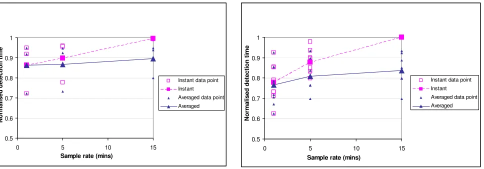
sensor. Figures 2a and 2b provide a comparison of these results at different sample rates for
instantaneous vs. averaged data for flow and pressure respectively.
{Figure 2a and 2b goes approximately here}
The figures illustrate an upward trend, i.e. that faster sampling leads to faster detection. Also, the use
of averaged data is faster than instantaneous data, improving as the sampling interval decreases.
Overall, averaged data has an improved detection time over instantaneous data, hence the
instantaneous 15 minute data is used as a reference datum. These improvements in detection times
are summarised in table 1 (with current industry practice cells shaded) and it is evident that
averaging can result in a more rapid detection time when compared to using the same instantaneous
sampling rate. Note that the 15 minute instantaneous entry appears as zero in the table as this was
used as the baseline.
DISCUSSION
The overall trend in the results is that faster sampling rate leads to earlier event detection. It is
important to note that faster sampling may also lead to slightly more ghost detections (false
positives) depending on parameters chosen. Figure 3 illustrates this general trend for the study.
{Figure 3 approximately here}
It was discovered that averaging can result in a more rapid detection for the SVR methodology when
compared to using the same instantaneous sampling rate. Hence, we could conclude that averaging is
a useful strategy for both flow and pressure when dealing with fifteen minute data. A note of caution
should be applied in that one reason for the earlier detections is likely to be an artifact of the SVR
technique. The standard deviation of the training data (which is used to determine whether a value is
a surprise or not) is calculated from the averaged data. Since the variability of the averaged data is
less than the raw data, basing the standard deviation on the averaged data and not the raw data makes
a surprise more likely using the SVR technique which may result in more ghosts (results in figure 3
show instantaneous results having 19% fewer ghosts). However, in practice, the data averaging is
performed on the sensor so the instantaneous data would not be available directly.
The use of hydraulic models for operational decisions requires well calibrated models with small
errors which reflect as closely as possible the actual behaviour of the system, this becomes even
more critical for real-time modelling (Machell et al., 2010). Pressure measurements must provide
calculation of accurate friction loss components in order that an accurate representation of the flow
be small in comparison with the total head. However, any error in the measurement of total head will
be reflected in the implied friction loss, potentially leading to large errors in the network hydraulic
solution. Time-averaging accurate, higher frequency pressure data over consecutive time periods has
the potential to eradicate errors associated with short-term variations in pressure leading to more
accurate model calibration. This is readily possibly, allowing for suitable firmware upgrade, as
sensors already perform this for flow. Although this is sometimes utilised for temporarily deployed
logging (e.g. for leak surveys or data for model calibration) this is not the case for permanent
installations. It should be noted that the benefits reported here pertain to event detection and do not
necessarily apply to other applications such as real-time hydraulic state estimation.
CONCLUSIONS
• This investigation has shown that averaging is a useful strategy for both flow and pressure
data collected from water distribution systems for event detection. In particular, averaging on
the sensor (achievable without any additional overheads on communications by a simple low
cost firmware upgrade) is recommended for pressure data, with the following significant
benefits:
o Improved detection time over instantaneous data when using data for event detection
software (table 1)
o Eradication of errors associated with short-term variations in pressure leading to more
accurate hydraulic model calibration
o The likely provision of better regulatory compliance.
• It is concluded that, at the present time, a sampling interval of 1 minute (or 5 minutes) does
not significantly improve detection to the point were it is worth the added increase in power
Similarly, current online model approaches do not require data at these frequencies.
However, this is likely to change in the future as the density of sensing of water distribution
system parameters increases due to reducing costs and improving logging capacity and
communications options.
ACKNOWLEDGEMENTS
This work is part of the NEPTUNE project supported by the U.K. Engineering and Physical Science
Research Council, grant EP/E003192/1, and Industrial Collaborators. The authors would like to
thank Mr. Ridwan Patel and Mr. Lee Soady from Yorkshire Water Services and Dr. John Machell
from the University of Sheffield for their assistance in the fieldwork.
REFERENCES
Chang, C. C. and Lin, C. J. (2001) LIBSVM: a library for support vector machines, Software
available at http://www.csie.ntu.edu.tw/~cjlin/libsvm.
Khan, A., Widdop, P.D., Day, A.J, Wood, A.S., Mounce, S.R. and Machell, J. (2006) Artificial
Neural Network model for a low cost failure sensor: Performance assessment in pipeline distribution.
Transactions on Engineering, Computing and Technology. ENFORMATIKA, Vol. 15, pp 195-201,
ISSN 1305-5313.
Machell, J., Mounce, S. R. and Boxall, J.B. (2010) Online modelling of water distribution systems: a
UK case study, Drink. Water Eng. Sci., 3, pp.21-27.
Mounce, S.R. and Machell, J. (2006) Burst detection using hydraulic data from water distribution
Mounce, S. R., Boxall, J.B. and Machell, J. (2010a) Development and Verification of an Online
Artificial Intelligence System for Burst Detection in Water Distribution Systems. ASCE Water
Resources Planning and Management. Vol. 136, No. 3, pp. 309-318.
Mounce, S. R., Farley, B., Mounce, R. B & Boxall, J.B. (2010b). Field testing of optimal sensor
placement and data analysis methodologies for burst detection and location in an urban water
network. Proceedings of HydroInformatics conference 2010, Chemical Industry Press, Vol 2,
pp.1258-1265.
Mounce, S. R., Mounce, R. B and Boxall, J.B. (2010c) Novelty detection for time series data
analysis in water distribution systems using Support Vector Machines. Journal of HydroInformatics,
In Press.
Puust, R., Kapelan, Z., Savic, D. A. and Koppel, T. (2010). A review of methods for leakage
management in pipe networks, Urban Water Journal, 7(1), 25-45
Romano, M., Kapelan, Z. And Savic, D.A. (2010) Pressure signal de-noising for improved real-time
leak detection. In Proceedings of the 9th International Conference on Hydroinformatics, Chemical
Industry Press, Vol 3, pp.2195-2202.
Stoianov I., Karney B., Covas D., Maksimovi C. & Graham N. (2002). Wavelet Processing of
Transient Signals for Pipeline Leak Location and Quantification, 1st Annual Environmental and
Water Resources Systems Analysis (EWRSA) Symposium, A.S.C.E. EWRI Annual Conference,
Walski, T.M. (2000) Model calibration data: the good, the bad, and the useless J.AWWA, v92, n1,
January, pp. 94-99.
Wu, Z. Y., Farley, M., Turtle, D., Kapelan, Z., Boxall, J. B., Mounce, S. R., Dahasahasra, S., Mulay,
M. and Kleiner, Y. (2011) Chapter 9. “Online Monitoring and Detection” in Water Loss, pp.
168-189, Bentley Systems, Ed. Zheng Wu. ISBN: 978-1-934493-08-3.
Ye, G. and Fenner, R. (2010). Kalman Filtering of Hydraulic Measurements for Burst Detection in
Water Distribution Systems. ASCE Journal of Pipeline Systems Engineering and Practice. ISSN
Figure captions:
Figure 1: Pressure measured at five second intervals with five minute averaging and to a resolution
of 0.5m in a 100mm diameter pipe
Figure 2a: Average normalised detection times for instantaneous versus averaged data (flow)
Figure 2b: Average normalised detection times for instantaneous versus averaged data (pressure)
Figure 3: Average ghosts for differing sample intervals for averaged vs. instantaneous data across all
sensors
Table captions:
Table 1: Summary of average improvement in detection times minutes, relative to 15 minute
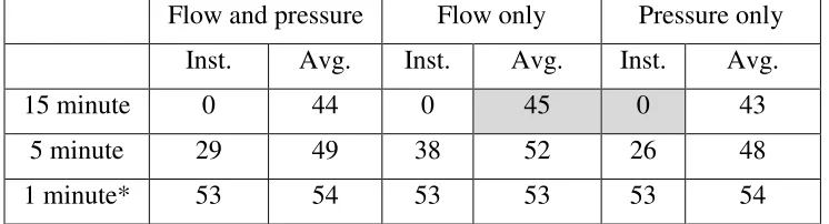
Table 1: Summary of average improvement in detection times (minutes), relative to 15 minute instantaneous data in each case.
Flow and pressure Flow only Pressure only
Inst. Avg. Inst. Avg. Inst. Avg.
15 minute 0 44 0 45 0 43
5 minute 29 49 38 52 26 48
1 minute* 53 54 53 53 53 54
*It should be noted that 1 minute was the minimum resolution for source flow data hence 1 minute instantaneous and average flow data are the same, however source data for pressure was available at 5 second resolution hence 1 minute averaged and instantaneous pressure data
are not the same.
Figures
58 59 60 61 62 63 64 65
0 300 600 900 1200 1500 1800 2100 2400 2700 3000 3300 3600 m
time (seconds) Pressure (5 second)
Instant (5 min) Averaged (5 min)
0.5 0.6 0.7 0.8 0.9 1
0 5 10 15
Sample rate (mins)
N or m a li s ed d e te c tio n ti me
Instant data point Instant Averaged data point Averaged 0.5 0.6 0.7 0.8 0.9 1
0 5 10 15
Sample rate (mins)
No rma li se d d e te ct ion t ime
Instant data point Instant Averaged data point Averaged
[image:18.595.61.545.154.323.2]Figure 2a: Average normalised detection times for instantaneous versus averaged data (flow)
Figure 3: Average ghosts for differing sample intervals for averaged vs. instantaneous data across all