White Rose Research Online
[email protected]
Universities of Leeds, Sheffield and York
http://eprints.whiterose.ac.uk/
This is the author’s post-print version of an article published in the
Proceedings
of the London Mathematical Society
White Rose Research Online URL for this paper:
http://eprints.whiterose.ac.uk/id/eprint/77023
Published article:
Marsh, RJ and Palu, Y (2013)
Coloured quivers for rigid objects and partial
triangulations: The unpunctured case.
Proceedings of the London Mathematical
Society. 1 - 29. ISSN 0024-6115
TRIANGULATIONS: THE UNPUNCTURED CASE
ROBERT J. MARSH AND YANN PALU
Abstract. We associate a coloured quiver to a rigid object in a Hom-finite 2-Calabi–Yau triangulated category and to a partial triangulation on a marked (unpunctured) Riemann surface. We show that, in the case where the category is the generalised cluster category associated to a surface, the coloured quivers coincide. We also show that compatible notions of mutation can be defined and give an explicit description in the case of a disk. A partial description is given in the general 2-Calabi–Yau case. We show further that Iyama-Yoshino reduction can be interpreted as cutting along an arc in the surface.
Introduction
Let (S, M) be a pair consisting of an oriented Riemann surfaceSwith non-empty boundary and a set M of marked points on the boundary ofS, with at least one marked point on each component of the boundary. We further assume that (S, M) has no component homeomorphic to a monogon, digon, or triangle. A partial triangulation R of (S, M) is a set of noncrossing simple arcs between the points in
M. We define a mutation of such triangulations, involving replacing an arcαofR
with a new arc depending on the surface and the rest of the partial triangulation. This allows us to associate a coloured quiver to each partial triangulation of M in a natural way. The coloured quiver is a directed graph in which each edge has an associated colour which, in general, can be any integer.
LetC be a Hom-finite, 2-Calabi–Yau, Krull-Schmidt triangulated category over a field k. Arigid object inC is an objectR with no self-extensions, i.e. satisfying Ext1C(R, R) = 0. Rigid objects inC can also be mutated. In this case the
muta-tion involves replacing an indecomposable summandX ofRwith a new summand depending on the relationship betweenX and the rest of the summands ofR. As above, this allows us to associate a coloured quiver to each rigid object of C in a natural way.
In [BZ] the authors study the generalised cluster categoryC(S,M)in the sense of
Amiot [Ami09] associated to a surface (S, M) as above. Such a category is triangu-lated and satisfies the above requirements. It is shown in [BZ] that, given a choice of (complete) triangulation of (S, M), there is a bijection between the simple arcs in (S, M) (joining two points inM), up to homotopy, and the isomorphism classes of rigid indecomposable objects inC(S,M). IfXαdenotes the object corresponding to
an arcαthen Ext1C(S,M)(Xα, Xβ) = 0 if and only ifαandβdo not cross. It follows
that there is a bijection between partial triangulations of (S, M) and rigid objects
Date: 24 May 2013.
2010Mathematics Subject Classification. Primary: 16G20, 16E35, 18E30; Secondary: 05C62, 13F60, 30F99.
Key words and phrases. Cluster category; quiver mutation; triangulated category; rigid object; coloured quiver; Riemann surface; partial triangulation; Iyama-Yoshino reduction.
This work was supported by the Engineering and Physical Sciences Research Council [grant number EP/G007497/1].
in C(S,M). Our main result is that the coloured quivers defined above coincide in
this situation and that the two notions of mutation are compatible.
Suppose thatαis a simple arc in (S, M) as above. LetXαbe the indecomposable
rigid object corresponding to α. Iyama-Yoshino [IY08] have associated (in a more general context) a subquotient category (C(S,M))Xα toXαwhich we refer to as the Iyama-Yoshino reduction of C(S,M)at Xα. The Iyama-Yoshino reduction is again
triangulated. We show that (C(S,M))Xα is equivalent toC(S,M)/α where (S, M)/α denotes the new marked surface obtained from (S, M) by cutting alongα.
By studying the combinatorics, we are able to give an explicit description of the effect of mutation on coloured quivers associated to a disk with n marked points. The corresponding cluster category in this case was introduced indepen-dently in [CCS06] (in geometric terms) and in [BMR+06] as the cluster category
associated to a Dynkin quiver of type An−3. We also give a partial explicit
de-scription of coloured quiver mutation in the general (2-Calabi–Yau) case, together with a categorical proof. In general, there are quite interesting phenomena: we give an example to show that infinitely many colours can occur in one quiver, and also show that zero-coloured 2-cycles can occur (in contrast to the situation in [BT09]). We remark that in the case of a cluster tilting object T in an acyclic clus-ter category the categorical mutation we define coincides with that considered in [BMR+06]; also with that in the 2-Calabi-Yau case considered in [BIRSc09,
Pal09]. It also coincides in the maximal rigid case considered in [GLS06, BIRSc09, IY08]. In this case, the coloured quiver we consider here encodes the same informa-tion as the matrix associated to T in [BMV10] provided there are no zero-coloured two-cycles. With this restriction, the mutation of this matrix coincides [BMV10, 1.1] with the mutation [FZ02] arising in the theory of cluster algebras. We note also that this fact for the cluster tilting case was shown in [BIRSc09] under the assumption that there are no two-cycles or loops (1-cycles) in the quiver of the endomorphism algebra; the cluster category case was considered in [BMR08] and the stable module category over a preprojective algebra was considered in [GLS06]. See also [BIRSm] and [KY11], where mutation of quivers with potential [DWZ08] has been studied in a categorical context. There has been a lot of work on this subject: see the survey [Kel10] for more details.
The geometric mutation of partial triangulations mentioned above specialises to the usual flip of an arc in the triangulation case (see [FST08, Defn. 3.5]). Coloured quivers similar to those considered here have been associated to m-cluster tilting objects in an (m+ 1)-Calabi-Yau category in [BT09] (in this case, the number of colours is fixed at m+ 1). The geometric mutation we define here should also be compared with the geometric mutation form-allowable arcs in a disk [BT09, Sect. 11]; see also the geometric model of the m-cluster category of typeAin [BM08].
We also note that the 2-Calabi-Yau tilting theorem of Keller-Reiten [KR07, Prop. 2.1] (see also Koenig-Zhu [KZ08, Cor. 4.4] and Iyama-Yoshino [IY08, Prop. 6.2]) was recently generalised [BM] to the general rigid object case, using Gabriel-Zisman localisation. This result suggests that the mutation of general rigid objects should be considered.
We note that some of our definitions and results could be generalised to the punctured case, except for that fact that we rely on results in [BZ] which apply only to the unpunctured case and are not yet known in full generality (see the recent [CIL-F]). Hence we restrict here to the unpunctured case.
that cutting along an arc corresponds categorically to Iyama-Yoshino reduction. In particular, the coloured quiver after cutting along an arc in a partial triangulation can be obtained from the coloured quiver of the partial triangulation by deleting a vertex. In Section 5 we show that, for a partial triangulation of a surface and the corresponding rigid object in the cluster category of the surface, the two notions of coloured quiver coincide. In Section 6 we show that mutation in the typeAcase can be described purely in terms of the coloured quiver and give an explicit description. We also give the example mentioned above in which the associated coloured quiver contains infinitely many colours. Finally, in Section 7, we give a partial explicit description and categorical interpretation of coloured quiver mutation. This last result holds in any Hom-finite, Krull-Schmidt, 2-Calabi–Yau triangulated category.
Acknowledgements Robert Marsh would like to thank Aslak Bakke Buan for some helpful discussions. Both authors would like to thank the referee for helpful comments which improved an earlier version of this article.
1. Preliminaries
1.1. Riemann surfaces. In this section, we recall some definitions and results from [FST08] and [LF09].
We consider a pair (S, M) consisting of an oriented Riemann surface with bound-ary Sand a finite setM of marked points on the boundary ofS, with at least one marked point on each boundary component. We refer to such a pair as a marked surface. We fix, once and for all, an orientation ofS, inducing the clockwise orien-tation on each boundary component.
Note that:
• We do not assume the surface to be connected.
• We only consider unpunctured marked surfaces.
We will always assume that (S, M) does not have any component homeomorphic to a monogon, a digon or a triangle.
Up to homeomorphism, each component of (S, M) is determined by the following data:
• the genusg,
• the number of boundary componentsb and
• the number of marked points on each boundary component {n1, . . . , nb}.
An arc γ in (S, M) is (the isotopy class relative to endpoints of) a curve in
S whose endpoints belong to M, which does not intersect itself (except possibly at endpoints) and which is not contractible to a point. The marked points on a boundary component divide it into segments, and we say that an arc isotopic to an arc along one of these segments is aboundary arc. The termarc will usually refer to a non-boundary arc.
The set of all (non-boundary) arcs in (S, M) is denoted byA0(S, M). Two arcs
are said to benon-crossingif their isotopy classes contain representatives which do not cross, i.e. their crossing number is zero. IfRis a collection of non-crossing arcs
in (S, M), we will denote byA0
R(S, M) the set of arcs in (S, M) which do not cross
any arc inR and which do not belong toR.
A partial triangulation of (S, M) is a collection of non-crossing arcs. A maximal collection of non-crossing arcs is called a triangulation. The numbern of arcs in any triangulation of a connected marked surface is given by the formula:
n= 6g+ 3b+c−6,
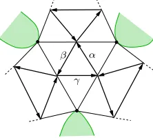
α β
[image:5.612.242.353.72.172.2]γ
Figure 1. The quiver with potential associated to a triangulated surface. The potentialW =αβγ+· · ·.
Let T be a triangulation. By [FST08, Sect. 4] and [LF09, Sect. 3] a quiver
Q = QT, together with a potential (a linear combination of cycles in QT up to
cyclic permutation)WT can be associated toT as follows. The vertices ofQ are
the arcs of the triangulation. There is an arrow from γ to γ′ for each triangle in
whichγ′ followsγwith respect to the orientation ofS, and the potentialW
T is the
sum of all the 3-cycles; see Figure 1, where part of a triangulated surface is shown. For an arrow a ∈ Q1, the cyclic derivative ∂a sends a cycle a1· · ·ad to the
sumPdk=1δakaak+1· · ·ada1· · ·ak−1. It is extended to potentials by linearity. The Jacobian algebra of the quiver with potential (QT, WT) is the quotient of the
complete path algebra kQ[T by the closure of the ideal generated by the cyclic
derivatives∂aWT, for alla∈Q1. We note that, by [CIL-F, Thm. 5.7], the Jacobian
algebra can, in this case, be taken to be the quotient of the path algebra kQT by
the ideal generated by the corresponding cyclic derivatives inkQT.
Theorem: LetT be a triangulation of a marked surface(S, M), and letT′ be the
triangulation obtained by flipping T at an arc γ. Then:
(a) [LF09, Thm. 36]The Jacobian algebraJ(QT, WT)is finite dimensional.
(b) [ABCJP10, Thm. 2.7]The Jacobian algebraJ(QT, WT)is gentle and
Goren-stein of GorenGoren-stein dimension 1.
(c) [FST08, Prop. 4.8]The quiver QT′ is given by the Fomin–Zelevinsky
mu-tation of QT at the vertex corresponding to γ.
(d) [LF09, Thm. 30]The quiver with potential(QT′, WT′)is given by the QP
mutation (see[DWZ08, Sect. 5]) of(QT, WT)at the vertex corresponding
toγ.
1.2. Cluster categories associated with Riemann surfaces. LetKbe a field. If C is a triangulated category, we will usually denote its shift functor by Σ. All the triangulatedK-categories under consideration in this paper are assumed to be Krull–Schmidt, Hom-finite (all morphism spaces are finite-dimensional K-vector spaces) and admit non-zerorigid objects (objectsR such thatC(R,ΣR) = 0). All rigid objects will be assumed basic (their summands are pairwise non-isomorphic). We will assume moreover that the triangulated categories are 2-Calabi–Yau, so that there are bifunctorial isomorphisms C(X,ΣY) ≃DC(Y,ΣX) for all objects X, Y, whereD is the vector space dualityD= HomK(−, K). A rigid objectT is called a
cluster tilting object if, in addition, for all objectsXinC,C(X,ΣT) = 0 =C(T,ΣX) implies that X belongs to addT.
1.2.1. Ginzburg dg algebras. Let (Q, W) be a quiver with potential (i.e. a QP). In this paper, we are mostly interested in QPs arising from triangulations of marked surfaces.
The Ginzburg dg-algebra Γ(Q, W) is defined as follows: First define a graded quiver Q. The vertices of Q are the vertices of Q, and the arrows are given as follows:
• the arrows ofQ, of degree 0;
• for each arrowαinQfromitoj, an arrowα∗ fromj toi, of degree−1;
• for each vertexiin Q, a loope∗
i ati, of degree−2.
The underlying graded algebra of Γ(Q, W) is the path algebra of the graded quiver
Q. It is equipped with the unique differentialdsending
• the arrows of degree 0 and each ei to 0; • the arrowα∗ to∂
αW, for eachα∈Q1, and
• the loope∗
i toei(Pα[α∗, α])ei, fori∈Q0.
The cohomology of Γ(Q, W) in degree zero is the Jacobian algebraJ(Q, W).
1.2.2. Generalised cluster categories. The cluster categories associated with acyclic quivers were introduced in [CCS06] in theAn case and in [BMR+06] in the acyclic
case. Amiot defined, in [Ami09], the generalised cluster categories, associated with quivers with potentials whose Jacobian algebra is finite dimensional.
Let (Q, W) be a quiver with potential such that the Jacobian algebra J(Q, W) is finite dimensional, and let Γ = Γ(Q, W) be the associated Ginzburg dg algebra.
LetDΓ be the derived category of Γ, and let DbΓ be the bounded derived
cat-egory. The perfect derived category per Γ is the smallest triangulated subcategory ofDΓ containing Γ and stable under taking direct summands.
Theorem[Kel09, Sect. 6]: The Ginzburg dg algebraΓis homologically smooth and 3-Calabi–Yau as a bimodule. In particular, there is an inclusion DbΓ⊂per Γ.
Definition[Ami09, Sect. 3]: The (generalised) cluster category C(Q,W) associated
with the quiver with potential (Q, W)is the Verdier localisationper Γ/DbΓ.
This definition is motivated by the following:
Theorem [Ami09, Sect. 3]: The cluster category C(Q,W) is Hom-finite and
2-Calabi–Yau. Moreover, the image of Γ in C(Q,W) is a cluster tilting object whose
endomorphism algebra is isomorphic to the Jacobian algebra J(Q, W). If Q is acyclic, then W = 0and the triangulated categoryC(Q,0) is equivalent to the acyclic
cluster category CQ=Db(Q)/τ−1[1]introduced in [BMR+06].
We also recall the 2-Calabi-Yau tilting theorem which applies in this context:
Theorem [KR07, Prop. 2.1] Let C be a triangulated Hom-finite Krull-Schmidt 2-Calabi-Yau category over a field K. If T is a cluster tilting object in C, then the functor C(T,Σ−) induces an equivalence between the category C/T and the category of finite dimensional EndC(T)-modules.
Note that the assumption in the paper that K be algebraically closed is not required for this result. We also note that this result has been generalised (see [IY08, Prop. 6.2], [KZ08, Sect. 5.1]).
1.2.3. Cluster categories from surfaces. Let (S, M) be a marked surface, and letT
be a triangulation of (S, M). Let (Q, W) be the quiver with potential associated withT. The following particular case of a theorem of Keller–Yang shows that the
be a triangulation of (S, M) obtained from T by a flip. Denote by (Q′, W′) the
associated quiver with potential.
Theorem [KY11]: There is a triangle equivalenceC(Q′,W′)≃ C(Q,W).
Since any two triangulations of (S, M) are related by a sequence of flips, the theorem above shows that the cluster categoryC(Q,W)is independent of the choice
of the triangulation T. The resulting category is denoted C(S,M) and is called
the cluster category associated with the marked surface (S, M). (We refer also to [BIRSm, Theorem 5.1]).
These categories have been studied by Br¨ustle–Zhang in [BZ]. We now recall those of their main results which will be used in the article.
Fix a triangulationT ={γ1, . . . , γm}of (S, M) with associated quiver with
po-tential (Q, W). LetT =T1⊕· · ·⊕Tmbe the image of Γ(Q, W) under per Γ(Q, W)→ C(Q,W)≃ C(S,M). Note that T is a cluster tilting object.
With each arcγnot inT is associated [ABCJP10, Proposition 4.2] an
indecom-posable J(Q, W)-module I(γ). Let Xγ be the unique (up to isomorphism)
inde-composable object in C(S,M) such that C(S,M)(T,ΣXγ) ≃I(γ). DefineXγk =Tk, fork= 1, . . . , m.
Theorem [BZ]:
• The mapγ7→Xγ is a bijection between the arcs of(S, M)and the
(isomor-phism classes of ) exceptional (i.e. indecomposable rigid) objects of C(S,M).
• For any two exceptional objectsXαandXβ, we haveExt1C(S,M)(Xα, Xβ) = 0
if and only if the arcs αandβ do not cross.
• The shift functor of C(S,M)acts on the arcs of(S, M)by moving both
end-points clockwise along the boundary to the next marked points.
Note that a bijection with these properties is not unique in general.
We note that our choice of an orientation of the Riemann surface differs from that of [BZ], but coincides with that of [BT09, Section 11].
We extend the bijection in the first part of the previous Theorem to a bijection between partial triangulations of (S, M) and rigid objects inC(S,M)in the obvious
way.
1.3. Iyama–Yoshino reduction. For an object X in a triangulated categoryC, we write⊥Xfor the full subcategory ofCwhose objects are those objectsY ofCsuch
that HomC(Y, X) = 0. The subcategoryX⊥ is similarly defined. For an additive
subcategory D of C, we write C/[D] for the quotient category whose objects are the same as the objects ofC with morphisms given by the morphisms ofC modulo those morphisms factoring through D. IfDis the additive closure of an objectX
in C then we just writeC/X forC/[D].
Theorem: [IY08, 4.2, 4.7] Let C be a2-Calabi-Yau triangulated category andR a rigid object in C. Then the subfactor category ⊥(ΣR)/R of C is again a 2
-Calabi-Yau triangulated category.
We refer to the subfactor category ⊥(ΣR)/R as the Iyama-Yoshino reduction
of C at R and denote it CR. We denote its shift by ΣR and the quotient functor
⊥(ΣR)−→ CRbyπ
R. See also [BIRSc09, II.2.1].
We recall a result of Keller:
Theorem: [Kel09, 7.4]LetQ, W be a quiver with potential whose Jacobian algebra is finite dimensional. Let i be a vertex of Q and let Pi be the image of the
atPi is triangle equivalent toC(Q′,W′), whereQ′ isQwith vertexi(and all incident
arrows) removed, and W′ isW with all cycles passing through ideleted.
2. Coloured quivers for rigid objects
2.1. Mutation and coloured quivers of rigid objects. LetK be a field. Let
Cbe aK-linear Hom-finite, Krull–Schmidt, 2-Calabi–Yau triangulatedK-category. LetR=R1⊕ · · · ⊕Rmbe a basic rigid object inCand letX be an indecomposable
rigid object inC Ext-orthogonal toR, i.e. such thatC(X,ΣR) = 0 =C(R,ΣX). Forc∈Z, consider triangles
X(c) f
c
−→B(c) g
c
−→X(c+1)−→ΣX(c)
where fc is a minimal left addR-approximation and gc is a minimal right addR
-approximation and where X(0) =X. These will be called the exchange triangles
for X with respect toR. They can be constructed using induction onc. We will often write κ(Rc)X forX(c), andκfor κ(1); κ
RX will be referred to as thetwist of
X with respect to R. Note thatκκ(c)=κ(c+1)=κ(c)κfor allc.
These exchange triangles lift the triangles X(c)−→0−→Σ
RX(c)−→ ΣRX(c)
in the Iyama–Yoshino reduction ⊥(ΣR)/R canonically to C. Therefore, X(c) is
indecomposable, rigid and Ext-orthogonal to addR for all c. This justifies the following definition:
Definition: The mutation of RatRk, for k∈ {1, . . . , m}, is the rigid object
µRkR=R/Rk⊕κR/RkRk. We will often writeµk forµRk and call it the mutation atk.
We note that our use of the work of Iyama–Yoshino to define the mutation above is similar to that of [BØO, Sect. 3] where cluster-tilting objects are mutated at a non-indecomposable summand.
In [BT09], the authors associate coloured quivers to d-cluster–tilting objects in (d+ 1)-Calabi–Yau categories. Here we use a similar definition to associate a coloured quiver to R.
For an integerd, we writeZ/dfor the quotient ofZby the ideal generated byd, identifying this with the set{0,1, . . . , d−1}ifd >0 and withZotherwise.
Definition: The coloured quiver Q = QR associated with the rigid object R is
defined as follows: The set of vertices is Q0={1, . . . , m}. We label each vertex k
with the periodicity dk(R)(possibly infinite) of the sequence of exchange triangles
for Rk. Fix two vertices i, j and c ∈ Z/di(R). Then the number q(c)(i, j) of c
-coloured arrows from i toj is given by the multiplicity ofRj inBi(c), where
R(ic) f
c i
−→Bi(c) g
c i
−→Ri(c+1)−→ΣRi(c)
are the exchange triangles as above forRi with respect toR/Ri.
Note that by definition,QR does not have any loops (1-cycles).
Remark:
• Analogous definitions would apply to a functorially finite, strictly full rigid subcategoryR of C closed under direct sums and direct summands, such that, for each indecomposable R ∈ R, the subcategory R \R is again functorially finite.
2.2. Mutation of rigid objects and Iyama–Yoshino reductions. The follow-ing lemma shows that the mutation of rigid objects is well-behaved with respect to Iyama–Yoshino reductions. This will turn out to be helpful in simplifying the proof of Theorem 18 in Section 7.
Let R =R1⊕ · · · ⊕Rm be a rigid object in C. Let CR = ⊥(ΣR)/(R) be the
Iyama–Yoshino reduction ofC with respect toR, with shift ΣR.
LetT be a rigid object inC, containingRas a direct summand. Assume thatTk
is a summand of T but not ofR, and consider the exchange triangle with respect to T /Tk:
(∗) Tk f −→B(0)k
g −→Tk(1)
ε −→ΣTk.
Here Bk(0) belongs to addT, where T=Tk⊕T.
Lemma 1. The induced morphismf is a minimal leftπR(T)-approximation inCR.
Proof. The triangle (∗) inC induces a triangle
Tk f
−→B(0)k −→g Tk(1)−→ΣRTk,
in CR. We have:
CR(Σ−R1πR(Tk(1)), πR(T))≃Ext1CR(πR(T
(1)
k ), πR(T))≃Ext1C(T
(1)
k , T) = 0,
using [IY08, Lemma 4.8]. Hence, the morphism f is a left πR(T)-approximation.
It is left minimal since Tk(1)is indecomposable inCR. √
Remark: Write Bk(0) =Rk(0)⊕Ck(0), with Ck(0) having no summands in common
with R. Then the morphismTk f′
−→Ck(0) is not a left T /R-approximation in C in
general.
Let Q be the coloured quiver of T in C, and let Q be the coloured quiver of
πR(T) inCR. Lemma 1 has the following immediate corollary:
Corollary 2. The coloured quiverQis the full subquiver ofQwith vertices corre-sponding to the indecomposable summands of T /R.
Moreover, computing the minimal T-approximation f ∈ C in the triangle (∗) amounts to computing the minimal add Tj-approximation of Tk in the Iyama–
Yoshino reductionCT /Tj for allj6=k. More precisely:
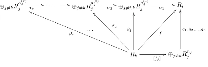
Lemma 3. LetR=R1⊕ · · · ⊕Rm be a rigid object inC and let1≤k≤m. For
each j = 1, . . . , m, let Cj denote the Iyama–Yoshino reduction of C with respect to
R/(Rk⊕Rj). Forj 6=k, letfj :Rk −→Rnjj be a map inCbe such thatRk fj
−→Rnj
j
is a minimal left addRj-approximation inCj. Then the morphism:
Rk
[fj]
−→M
j6=k
Rnj
j
is a minimal left addR/Rk-approximation inC.
Proof. Let i 6=k, and letRk f
−→ Ri be an arbitrary morphism in C. Sincefi is
an addRi-approximation in Ci, there are morphisms Lj6=kR nj
j g1
−→ Ri, Rk β1
−→
L
j6=i,kR a(1)j
j and
L
j6=i,kR a(1)j j
α1
−→Ri in C (for somea(1)j ) such that f =g1[fj] +
α1β1. Note that α1 must be a radical map, as no summand of its domain is
⊕j6=kR a(jr)
j αr //· · · //⊕j6=kR
a(2)j
j α2 //⊕j6=i,kR
a(1)j
j α1 //Ri
· · ·
Rk
[fj]
/ / βr h h RRRRRRRR RRRRRRRR RRRRRRRR RRRR RRRRRRR β2 ^ ^ >> >> >> >> >> >> >> >>> β1 O O f @ @
⊕j6=kRnjj g1,g2,...,gr
O
[image:10.612.134.466.76.184.2]O
Figure 2. Proof of Lemma 3
Reducing toCj for somej6=i, k, we see that the componentβ1,jofβ1 mapping
toRa (1)
j
j factors throughfj :Rk →Rjnj up to a map factoring through add⊕l6=j,kRl.
That is, we can writeβ1,j asujfj+wjvj for someuj:Rnjj →R a(1)j
j ,vj:Rk →Xj,
andwj :Xj →Rk, whereXj ∈add⊕l6=j,kRl. Note thatwj is a radical map, since
none of the summands inXj are isomorphic toRj.
Adding over all j for j 6= i, k, we obtain maps α2 : ⊕l6=kR a(2)l
l → ⊕j6=i,kR a(1)j
j ,
β2 : Rk → ⊕l6=kR a(2)l
l and γ2 : ⊕j6=kRnjj → ⊕j6=i,kR a(1)j
j (for some a
(2)
l ) such that
β1=α2β2+γ2[fj]. Setting g2=α1γ2we obtainα1β1=α1α2β2+g2[fj], so
f =g1[fj] +α1β1=α1α2β2+ (g1+g2)[fj].
Here, α2 is a radical map, since all of its summands, the wj, are radical. See
Figure 2.
Iterating this step we construct, for allr≥3, morphismsgr : Lj=6 kRnjj −→Ri,
αr : Lj6=kR a(jr)
j −→
L
j6=kR a(r−1)
j
j , and βr : Rk −→Lj6=kR a(jr)
j for r= 3, . . . n
(and some a(lr)), such thatf =βnαn· · ·α1+ (g1+· · ·+gn)[fj] and each of theαi
is a radical map. SinceC is Hom-finite, the radical of End(R) is nilpotent and the compositionβnαn· · ·α1vanishes fornbig enough. Thereforef factors through [fj]
and [fj] is a left addR/Rk-approximation inC. The left minimality of [fj] follows
from the left minimality of eachfj. √
3. Coloured quivers for partial triangulations
Let (S, M) be an unpunctured oriented Riemann surface with boundary and marked points. We will always assume that each boundary component contains at least one marked point and that no component of (S, M) is a monogon, a digon or a triangle.
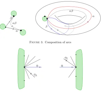
3.1. Composition of arcs. Let α and β be two oriented arcs in (S, M) with
β(1) =α(0). The compositionαβ is the arc given by
t7−→
β(2t) if 0≤t≤1/2
α(2t−1) if 1/2≤t≤1.
See Figure 3.
Note that the composition only makes sense for oriented arcs.
α β
αβ
α
β
[image:11.612.131.466.65.381.2]αβ
Figure 3. Composition of arcs
α α
αs
αt
Figure 4. Orientation ofαsandαt
LetR be a partial triangulation of (S, M), i.e. a collection of non-crossing arcs
γ1, . . . , γm. Let αbe an arc in (S, M) which does not crossRand does not belong
to R, i.e. α∈ A0
R(S, M). We define the twist ofα with respect to R as follows:
Choose an orientationαofα. Consider the arcs of the partial triangulationRwhich
admit α(0) as an endpoint. Restrict to a neighbourhood ofα(0) small enough not to contain any loop. The orientation of the boundary containing α(0) induces an ordering on the parts of the arcs included in the neighbourhood (see Figure 4). Let
αs be the arc, in R or boundary, which followsαin this ordering (note that it is
not allowed to beαitself). Similarly, define αtwith respect to the endpoint α(1).
These will be called thearcs following αinR.
We giveαsand αt the orientationsαs andαtdescribed in the local pictures of
Figure 4. Note that this orientation coincides with the orientation of the boundary ifαsorαtis a boundary arc.
For an oriented arcβ, let [β] denote the underlying unoriented arc. Define the twist of the arcα with respect to R to be the underlying unoriented arc of the
composition:
κR(α) = [αtα αs−1].
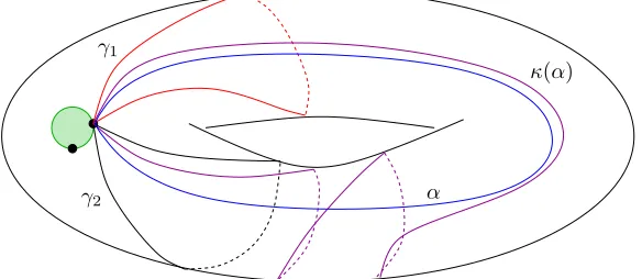
See Figure 5 for an example of a twist. Note that the definition of the arcκR(α)
does not depend on the choice of an orientation for α. It is easy to check, using a case-by-case analysis depending on whether or not α, αs, αt are loops and the
order in which they appear at their end-points, thatκR(α) does not cross any arc
in R, i.e. thatκR(α)∈A0
R(S, M).
The twist with respect to R is invertible with inverse κ−1
R , which can also be
α
κ(α)
γ1
[image:12.612.153.445.74.201.2]γ2
Figure 5. An example of a twist
3.3. Mutation of partial triangulations. Let R be a partial triangulation of
(S, M), and letβ∈R. WriteR=R⊔ {β}. Themutation ofRatβ is the partial
triangulation
µβR=R⊔κR(β) .
If R is a triangulation, then, for β ∈ R, µβR is the usual flip of R at the arc
β ∈R; see [FST08, Defn. 3.5].
3.4. Coloured quivers. Let R be a partial triangulation andα an arc which is
not an element of R and does not crossR. Let β be an arc inR. For allc∈Z,
define the numbers m(Rc)(α, β) by:
mR(α, β) =
2 ifβ =αs=αt
1 ifβ ∈ {αs, αt} andαs6=αt
0 otherwise,
m(Rc)(α, β) = mR(κcR(α), β).
We associate a coloured quiverQRwith a partial triangulationR={γ1, . . . , γm}
in the following way:
DefinitionThe coloured quiver QR associated with the partial triangulation R is
defined as follows: The set of vertices is Q0 ={1, . . . , m}. We label each vertex i
with the smallest integer d =di(R) such that κRd\γi(γi) =γi, or with zero if no such integer exists. Fix two distinct verticesi, j andc∈Z/di(R). Then the number
q(c)(i, j)ofc-coloured arrows from vertexito vertexj is given bym (c)
Ri(γi, γj), where Ri=R\ {γi}.
Note that QR, by definition, contains no loops. For an example of a coloured
quiver associated to a partial triangulation of a torus and the effect of mutation on the quiver, see Section 6.2.
4. Cutting along an arc and CY reduction
Let (S, M) be as in Section 3.
loop, then each endpoint ofαgives rise to two distinct marked points in (S, M)/α. Ifαis a loop, its endpoint gives rise to three distinct marked points in (S, M)/α.
The resulting marked surface cannot contain a monogon as a connected com-ponent, since αis not homotopic to a point. No connected component can be a bigon, since αis not a boundary arc. If a component homeomorphic to a triangle has been created, we remove it.
There is a natural bijection between the arcs on (S, M)/αand the arcs of (S, M) which do not cross the arc α. Moreover, the (partial) triangulations of (S, M)/α
correspond, through this bijection, to the (partial) triangulations of (S, M) con-taining the arc α.
Remark 4. The surface (S, M)/α can also be constructed as follows. LetT be a
triangulation of(S, M)containingα. The surface(S, M)is then obtained from the triangles of the triangulation by gluing matching sides of triangles in a prescribed orientation. The surface(S, M)/αis obtained from the same triangles by respecting the same gluings except for the sides which correspond to α, which are not glued together anymore.
Given a collection R of non-crossing arcs, one can cut successively along each
arc. Whatever order is chosen yields the same new surface, by Remark 4. The corresponding surface will be called the reduction of (S, M) with respect to R,
and will be denoted by (S, M)/R. We will denote the natural bijection between
A0
R(S, M) andA0((S, M)/R) byπR.
4.2. Compatibility with CY reduction. LetRbe a basic rigid object inC(S,M),
and let Rbe the associated partial triangulation. We denote byCR=⊥(ΣR)/(R)
the Calabi–Yau reduction ofC(S,M)with respect toR, and by (S, M)/Rthe marked
surface obtained from (S, M) by cutting along the arcs ofR.
Proposition 5. The triangulated categories C(S,M)/R andCR are equivalent.
Proof. Complete the collection of arcsR to a triangulationT. Let (Q, W) be the
QP associated withT. By definition, there is an equivalence of triangulated
cate-goriesC(S,M)≃ C(Q,W). By [Kel09, Theorem 7.4] (see section 1.3), the categoryCR
is triangle equivalent to the cluster category C(Q′,W′), where (Q′, W′) is obtained
from (Q, W) by deleting the vertices of Qwhich correspond to arcs in R, and all
adjacent arrows. On the other hand, the arcs in T not in R induce a
triangula-tion of the surface (S, M)/R. It follows from Remark 4 that (Q′, W′) is the QP
associated with this triangulation. ThusC(S,M)/R is equivalent toC(Q′,W′). √
Remark: Lemma 7 shows that the equivalence above is well-behaved with respect to well-chosen bijections between arcs and exceptional objects.
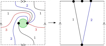
Figure 6 shows the effect of cutting along an arc in a triangulation of a torus with a single boundary component containing two marked points. We cut along the red arc (numbered 3) and obtain a cylinder with four marked points as shown, with triangulation given by the remaining arcs. In the last step, the cylinder has been rotated around to get a simpler picture. The effect on the corresponding quiver with potential is shown in Figure 7.
Proposition 6. Let (S, M) be a marked surface andR a partial triangulation of
(S, M). Let R′ be a collection of arcs containing R. Then the coloured quiver
associated toπR(R′\R)in(S, M)/Rcoincides with the coloured quiver associated
to R′ in (S, M) with the vertices corresponding to R and all arrows incident with
1 1 1 1 1 1 1 1 1 1 1 1 1 1 2 2 2 2 2 2 2 2 2 3 3 3 3 4 4 4 4 4 4 4 4 4 4 4 5 5 5 5 5 5 5 5 5 5 5
Figure 6. Cutting along an arc, numbered 3, in a torus to get a cylinder: triangulation case.
4 2 o o / / / / / / /
/ 4 2
/ / / / / / / / o o
• • 7→ •
3 //1
W W // // // // G G 5 o o 1 W W // // // // G G 5 o o
Figure 7. The change in the quiver with potential from the cut in Figure 6. The potential in each case is given by the sum of the 3-cycles containing black dots.
Proof. It is clear that the vertices of each coloured quiver correspond to the arcs in R′ \R. In the definition of the twist κR (see Section 3.2), no distinction is
made between arcs inR and boundary arcs. Then, looking at the definition of the
coloured quiver of a partial triangulation (see Section 3.4) we see that the arrows between arcs in R′\R are the same when considered in either coloured quiver.
The result follows. √
[image:14.612.192.407.369.428.2]1 1
1
1
2 2
2
[image:15.612.190.407.70.165.2]3 3
Figure 8. Cutting along an arc in a torus to get a cylinder: partial triangulation case.
(0,0)
(0,1) (0,1)
(0,1)
(1,2) (1,2)
(1,2) (2,2)
3 3
3
3 3
1 1
2 2
3
Figure 9. The effect of cutting along arc 3 on the coloured quiver of the partial triangulation in Figure 8. The vertices themselves are encircled, with the vertex labels written outside the circle.
5. Compatibility
5.1. Compatibility of the mutations. LetR={γ1, . . . , γm}be a partial
trian-gulation of (S, M). CompleteR to a triangulationT of (S, M), and letT be the
associated cluster tilting object inC=C(S,M). LetRbe the direct summand of T
corresponding to R. We thus obtain a map α7→ Xα between the arcs of (S, M)
and the isomorphism classes of exceptional objects in C(S,M) (see section 1.2.3).
We denote by πR the bijection A0R(S, M) → A0 (S, M)/R
; recall also that πR
denotes the functor ⊥(ΣR) → CR. Consider the partial triangulation π
R(T \R)
of (S, M)/R. Note thatT′ :=πR(T) is cluster tilting in C(S,M)/R≃ CRby [IY08,
Theorem 4.9]. This cluster tilting object induces a bijection β 7→Yβ between the
arcs in (S, M)/Rand the exceptional objects inCR.
Lemma 7. Let α be an arc in A0
R(S, M). Then the image of Xα under πR is
isomorphic to YπRα.
Proof. Using [JP, Proposition 3.5], the modules associated with πRXα and YπRα
are seen to be isomorphic. √
Let αbe an arc in (S, M) which is not in R and which does not cross R, i.e.
α∈A0
R(S, M). Fix an orientation αofαand let αs and αtbe the two (possibly
boundary) arcs following αin R (as defined in section 3.2). Recall that κR(α) is
defined to be [αtααs−1].
Ifγ is any arc in (S, M) then recall we have (from [BZ]; see Section 1.2.3):
(1) ΣXγ =Xκφ(γ),
where φdenotes the empty set of arcs in (S, M). Thusκφ(α) is obtained from the
[image:15.612.160.441.213.330.2]The following corollary describes the twist of an arc in terms of the action of the shift functor of an Iyama-Yoshino reduction.
Corollary 8. Under the bijectionA0
R(S, M)↔A0 (S, M)/R
, the induced action of the shift functor of C(S,M)/R on A0R(S, M) coincides with that of the twistκR.
In other words, we have a commutative diagram:
A0 (S, M)/R shift //A0 (S, M)/R
A0
R(S, M)
πR
O
O
κR
/
/A0
R(S, M).
πR
O
O
Proof. Letα∈A0
R(S, M). By (1), noting thatRbecomes part of the boundary of
(S, M)/R, we have ΣRYπR(α)≃Yπ
RκR(α). The result follows.
√
We now have the ingredients we need in order to show that the two mutations (of partial triangulations and rigid objects) are compatible.
Proposition 9. Let R = R1⊕ · · · ⊕Rm be the rigid object in C(S,M) associated
with the partial triangulation R as above. Fix 1 ≤ k ≤ m. Then we have the
indecomposable summandRk ofR and corresponding arcγk ofR. Letαbe an arc
in A0
R(S, M). Then we have:
κRXα≃XκR(α) andµkR≃XµkR.
Hence, in particular, dk(R) =dk(R).
Proof. Since α does not cross R, it follows from [BZ] (see Section 1.2.3) that
Xα∈⊥(ΣR). Similarly, XκR(α) ∈⊥(ΣR), sinceκR(α) does not crossR. By the
description of the shift ΣRofCRin [IY08, 4.1],πR(κR(Xα))≃ΣR(πRXα) inCR. By
Lemma 7, ΣR(πRXα)≃ΣRYπR(α). By Corollary 8, we have ΣRYπR(α)≃YπRκR(α).
By Lemma 7,YπRκR(α)≃πRXκR(α). HenceπR(κRXα)≃πR(XκR(α)).
Note that κRXα is an indecomposable object in ⊥(ΣR) which is not in addR
(see Section 2.1). Since κR(α) does not cross R and does not lie in R, the same
is true of XκR(α). It follows that κRXα ≃ XκR(α), proving the first part of the
Proposition. The second and third statements follow. √
5.2. Compatibility of the coloured quivers. As in the previous section, let
α∈A0
R(S, M); we fix an orientation of αand let αs and αt be the two (possibly
boundary) arcs followingαinR(as defined in section 3.2). Note that it is possible
that αs=αt. We choose a triangulationT of (S, M) containingRand α. Let T
be the corresponding cluster tilting object, containingRas a direct summand and
Xαas an indecomposable direct summand. Recall that Xγ = 0 if γis a boundary
arc.
Lemma 10. There is a minimal left addR-approximation of Xα inC(S,M) of the
form
Xα−→Xαs⊕Xαt.
Proof. By the 2-Calabi-Yau tilting theorem (see Section 1.2.2), the functor H =
C(T,Σ−) induces an equivalence betweenC/T and modJ(Q, W). HenceHinduces an equivalence between Σ−1addT and the category P of projective modules over
J(Q, W). Let Pα=H(Σ−1Xα) for each arcαin T and letPR=H(Σ−1addR).
Then it is enough to show that there is a minimal leftPR-approximation ofPα in
modJ(Q, W) of the form
We recall that J(Q, W) is gentle (see Section 1.1). In particular, the defining relations are all zero-relations. Letδ1, δ2, . . . , δjbe the arcs inT incident withα(0)
which are after αin the order induced by the orientation of the boundary atα(0) (and listed in that order); see Section 3.2. Similarly, let ε1, ε2, . . . , εk be the arcs
in T aroundα(1) which are afterαin the order induced by the orientation of the
boundary atα(1).
Because of the zero-relations inJ(Q, W), the only non-zero paths in Qstarting at αare paths:
α−→δ1−→δ2−→ · · · −→δj
and
α−→ε1−→ε2−→ · · · −→εk.
Thus the only non-zero morphisms from Pα to some indecomposable projective
module lie in the composition chains:
Pα−→Pδ1 −→Pδ2 −→ · · · −→Pδj
and
Pα−→Pε1 −→Pε2−→ · · · −→Pεk,
or are linear combinations of these (noting that the chains may overlap).
If αt is a boundary arc, but αs is not, thenαs occurs in the first chain above.
It is easy to see that the non-zero map Pα −→ Pαs coming from the chain of compositions is a left minimalPR-approximation and we are done. The argument
is similar if αs is a boundary arc butαt is not. If both αs and αt are boundary
arcs then the zero map is a left minimal PR-approximation.
We are left with the case where neitherαsnorαtis a boundary arc. Thusαs=δi
for some i while αt = εi′ for some i′. Let fs and ft be the non-zero morphisms
arising from the above chains of compositions and let f : Pα −→ Pαs ⊕Pαt be the map with components fs, ft. It follows from the above that f is a left PR
-approximation ofPα. It remains to check thatf is left minimal.
We note that if we had fs=khfor someh:Pα−→Pβ andk:Pβ −→Pαs for someβ ∈R thenkwould have to be an isomorphism since the path in Qfrom α
toαsis not equal to any other path inQfromαtoαs, andαsis the first arc inR
appearing along this path. A similar statement holds forft.
Iffwere not left minimal, a summand of form 0−→Pαs(respectively, 0−→Pαt) would split off and we would have a leftPR-approximation of the formgs:Pα−→
Pαs (respectively,gt:Pα−→Pαt). We consider only the first case (the second case requires a similar argument). In this case, ftfactors through gs, i.e. ft =vgsfor
some mapv:Pαs→Pαt. By the above,v is an isomorphism andgs=v
−1f
t.
Again, sincegsis a leftPR-approximation, we also have thatfsfactors through
gs, i.e. fs =wgs for some w:Pαs −→Pαt. By the above, w is an isomorphism. Hence we havefs=wv−1ftwherewv−1is an isomorphism. This is a contradiction
sincefsandftarise from two different paths starting atα. The result is proved. √
Theorem 11. Let Rbe the rigid object inC(S,M)associated with the partial
trian-gulation R. Then the coloured quivers QR andQR coincide.
Proof. By Proposition 9, it is enough to prove that the sets of 0-coloured arrows
coincide. This follows from Lemma 10. √
6. Some examples
6.1. The An case. In this section, we assume that the category C is the cluster
category of typeAn.
Suppose that R = R1⊕ · · · ⊕Rm is a basic rigid object in C. In Section 2.1
α β
Figure 10. The arc α has order 3 under twisting and lies in a hexagon, while the arcβ has order 5 and lies in a pentagon.
summand ofR then the rigid objectµkRalso has a coloured quiver,Qe, associated
with it, and we can ask if Qe can be computed from Q. This is known in the d -cluster-tilting object case of a d+ 1-Calabi-Yau category [BT09, Thm. 2.1] but is not known for a general rigid object. In Section 7 we will indicate some results in this direction with a categorical proof, but here we give a complete answer for the cluster category of type A using a combinatorial (geometric) proof. In this case, the corresponding surface is a disk withn+ 3 marked points (see [CCS06]), which we shall denote (S, M); as usual, we denote by R the set of noncrossing arcs in
(S, M) corresponding to the indecomposable direct summands ofR, writingγifor
the arc corresponding to Ri. We may assume that all arcs are straight lines. We
have seen above that we can computeQusingR instead ofR.
If R is indecomposable, the corresponding coloured quiver is trivial (a single vertex and no arrows) and there is nothing more to do. We assume we are not in this case.
The complement in (S, M) of R\ {γi} is a union of disks, including one, Di,
containingγi, with a polygonal boundary. Then, by its definition,κR\{γi} has the effect of rotating each of the endpoints of γi anticlockwise one edge around the
polygonal boundary ofDi.
If the boundary of Di is a polygon with an even number of sides andγi joins
two opposite vertices on this boundary then we say that γi issymmetric.
Lemma 12. The arc γi is symmetric if and only if, for any vertex j such that
i and j are ends of a common arrow in Q, there is a unique colour c such that
q(c)(i, j)6= 0.
Proof. Let Di be the disk defined above. If γi is symmetric, then the minimum
number of twists with respect to R\γi required to return γi to itself is equal to
half the number of sides of the boundary of Di and this has the effect of rotating
γi through half a revolution. It follows that ifiandj are ends of a common arrow
in Q, there is a unique colour c such that q(c)(i, j) 6= 0. If γi is not symmetric,
the minimum number of twists required is equal to the total number of sides of the boundary ofDi, and this has the effect of rotatingγi through a full revolution. We
see that ifiandj are ends of a common arrow inQ, there are exactly two distinct
coloursc such thatq(c)(i, j)6= 0. √
We remark that a vertexj as in Lemma 12 always exists, since we have assumed that Rhas more than one element. It follows that whetherγi is symmetric or not
is determined by the coloured quiverQ. See Figure 10 for an example. We have the following:
Lemma 13. Fix i ∈ {1,2, . . . , m}. Choose a vertexj such thatq(c)(i, j)6= 0 for
r
s t
[image:19.612.238.358.65.188.2]i j
Figure 11. Proof of Lemma 13.
Then we have:
di= max{c≥0 : q(c)(i, j)6= 0}+ min{c≥0 : q(c)(j, i)6= 0}+ 1.
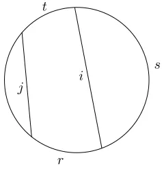
Proof. Suppose first thatγiis not symmetric. Then the situation is as in Figure 11,
where the labels on the boundary indicate the number of edges along sections of the boundary. Sincedi is the number of sides ofDi, we have that
di= (s+t) +r+ 1 = max{c≥0 : q(c)(i, j)6= 0}+ min{c≥0 : q(c)(j, i)6= 0}+ 1.
as required. If γi is symmetric, then di is half the number of sides of Di. The
situation can again be depicted as in Figure 11 (with the additional restriction that
t+r+ 1 =s) and we obtain:
di =t+r+ 1 = max{c≥0 : q(c)(i, j)= 06 }+ min{c≥0 : q(c)(j, i)6= 0}+ 1.
√
The possibility of symmetric arcs makes it difficult to compute the new coloured quiver after mutation of R at an arc, so we use a modified version of the original
quiver, defined as follows.
DefinitionThemodified coloured quiver Q+R ofR is the coloured quiver obtained
from QR as follows. The vertices are{1,2, . . . , m}. We set
d+i (R) = (
2di(R), ifγi is symmetric;
di(R), ifγi is not symmetric.
If γi is symmetric, we set q+(c)(i, j) =q(c)(i, j) and q(+c+di)(i, j) = q(c)(i, j) for all
c∈ {0,1, . . . , di−1}, while ifγiis not symmetric, we setq(+c)(i, j) =q(c)(i, j) for all
c∈ {0,1, . . . , di−1}.
Note that for any two distinct vertices i and j, the modified coloured quiver always has exactly two arrows fromito j. We usually write this as a single arrow labelled with the two colours (l, l′), withl≤l′. We also note that the arrows inQ+
R
can be obtained from R using the same rules (see Section 3.4) as for QR except
that we use the numbers d+
i (R) instead of the numbers di(R). Using the same
arguments as in the proof of Lemma 13, we have (again choosing a vertex j such that q+
(c)(i, j)6= 0 for somec):
(2) d+i = max{c≥0 : q(+c)(i, j)6= 0}+ min{c≥0 : q +
(c)(j, i)6= 0}+ 1.
Lemma 14. The modified coloured quiver ofRis determined by the coloured quiver
i i
i i
k k
k
k
p p
q−1
q
r+ 1
r
(r,r+p)
(0,q)
(0,p)
(q−1,q+r)
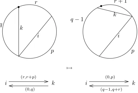
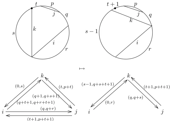
[image:20.612.184.414.70.226.2]7→
Figure 12. Case I. Here we have p≥2,q≥2,r≥1. Note that
d+i =p+r+ 1, ˜d+i =p+qandd+k = ˜d+k =q+r+ 1.
Proof. Given the coloured quiverQR ofR, Lemma 12 indicates how to determine
which arcs are symmetric, and thus how to computeQ+Rdirectly fromQRusing the
definition above. Note that an arcγiis symmetric if and only ifd+i =d+i (R) is even
and there is a vertexj and a colourcsuch thatq+(c)(i, j)6= 0 andq+
(c+1 2d
+
i)
(i, j)6= 0. It follows that the coloured quiver of R can be determined from the modified
coloured quiver of R. √
It is thus enough for us to give a method for determining the modified coloured quiver of the mutation of a rigid object in terms of the modified coloured quiver of the rigid object. We first compute the change in the quiver in a number of cases.
Figures 12–16 each show a configuration of arcs in (S, M), together with the result after mutation atγk. In each case, a label on part of the boundary indicates
the number of boundary edges between the two nearest arc ends on the boundary and the black dot indicates the end of arckto show how this has changed after the mutation. The following is a simple calculation:
Lemma 15. For each of the five cases in Figures 12–16, the effect of mutation at
k on the corresponding modified coloured quiver is as shown.
We next consider, in the general case, the effect of mutation at a vertex k on the modified coloured quiverQ+=Q+
R. Letk∗be the set of vertices at the targets
of arrows starting at k with colour zero. A vertexi lies in k∗ if and only if γ
i is
incident with a single endpoint of γk and the clockwise angle from γk and γi is
inside (S, M); see the diagram on the left hand side of Figure 12, where i is an example of an element ofk∗.
Suppose i6∈k∗ and that there is an arrow from i to kin Q+. Then neither of
the colours in the label of the arrow is equal tod+
i −1 (elseiwould lie ink∗). The
effect of mutating atkis to increase both of these colours by 1. If there is an arrow from k toi in Q+ then, for the same reason, the colours in the label of the arrow
are non-zero and mutation at kdecreases these by 1.
Ifi∈k∗, then the effect onQ+ of mutating atkis shown in Figure 12: the disk
in this picture should be interpreted as the boundary of the connected component of the complement in (S, M) ofR\ {γi, γk} containingγi andγk.
Mutation at k can only affect the vertex labels corresponding to arcs on the boundary of the connected component of the complement in (S, M) of the arcs in
i i
i i
j j
j j
k
k
k
k p
p
q−1
q r r+ 1
s s
t t
(t,p+t)
(t,p+t) (q,q+r+1)
(r,r+s) (0,q+t+1)
(q,q+s)
(t+1,p+t+1)
(q−1,q+r) (q+t,q+r+t+1)
(0,s)
[image:21.612.169.440.67.273.2]7→
Figure 13. Case II. Here we havep≥2,q≥1,r≥1,s≥2,t≥0. Note thatd+i =r+s+ 1, ˜d+i =q+t+s+ 1,d+j = ˜d+j =p+q+t+ 1
andd+k = ˜d+k =q+r+t+ 2.
i
i i
i
j j
j j
k
k k
k
p p
q q
r r
s s−1
t t+ 1
(t,p+t)
(q+1,q+s+1) (0,s)
(q+t+1,q+r+t+1)
(t+1,p+t+1)
(t+1,p+t+1)
(q,q+r)
(q,q+s) (s−1,q+s+t+1)
(0,r)
7→
Figure 14. Case III. Here we havep≥ 2,q ≥0, r ≥2, s ≥2,
t≥0. Note thatd+i =q+r+t+2, ˜d+i =r+s,d+j = ˜d+j =p+q+t+2 andd+k = ˜d+k =q+s+t+ 2.
We observe that mutation at k can only affect arrows in Q+ incident with k
(already considered above) or incident with at least one vertex ink∗.
Consider first the arrows between vertices i ∈ k∗ and j 6∈ k∗. Figures 13, 14
and 15 show the three possibilities for the location ofγj. In each case the disk should
be interpreted as the boundary of the connected component of the complement in (S, M) of the arcs inR\ {γi, γj, γk} containingγi, γj andγk.
[image:21.612.159.446.338.543.2]i
i
i
i
j j
j j
k
k k
k
p p
q q
r r−1
s s+ 1
t t
(t,p+t) (t,p+t) (q,q+s+1)
(0,r)
(s,q+s+t+1)
(r−1,r+s)
(q,q+r) (0,q+t+1)
[image:22.612.162.434.68.267.2]7→
Figure 15. Case IV. Here we have p≥2, q ≥0, r ≥2, s ≥1,
t≥0,q+t≥1. Note thatd+i =q+s+t+ 2, ˜d+i =q+r+t+ 1,
d+j = ˜d+j =p+q+t+ 1 andd+k = ˜d+k =r+s+ 1.
i1
i1
i1
i1
i2
i2
i2
i2
k k k
k
p p
q q
r r
s s
(q,q+s+1) (0,r)
(0,p) (s,q+s+1)
(s,p+s)
(0,q+1) (0,s+1)
(q,q+r)
7→
Figure 16. Case V. Here we havep≥2,q≥1,r≥2,s≥1. Note thatd+i1 =q+r+ 1, ˜d+i1 =r+s+ 1,d+i2 =p+s+ 1, ˜d+i2 =p+q+ 1 andd+k = ˜d+k =q+s+ 2.
Finally, we consider the arrows between vertices i1, i2∈k∗. This case is shown
in Figure 15, with the disk interpreted as the boundary of the connected component of the complement in (S, M) of the arcs inR\ {γi1, γi
2, γk}containingγi1, γi2 and γk. The effect of mutation on the corresponding full subquiver ofQ+ is as shown.
Analysing the effect of mutation leads us to the following method for mutating a (modified) coloured quiver in type A.
Proposition 16. Let R=R1⊕ · · · ⊕Rm be a rigid object in the cluster category
of type An, with associated modified coloured quiver Q+. Let Rk be a summand
of R and let Qe+ denote the modified coloured quiver ofµ
[image:22.612.157.438.329.526.2]associated to vertex i. ThenQe+ can be computed in the following way. The letters
i, j, k always refer to distinct vertices.
Type A modified coloured quiver mutation:
(i) Suppose we have the following arrows:
i
(a,a′)
/
/
k
(0,b′)
o
o j
(c,c′)
/
/
k
(d,d′)
o
o
whered6= 0. Add the following arrows:
i
(d,d+a′−a)
/
/j
(c,c′)
o
o
and cancel any pairs of arrows betweeniandj in the same direction whose colours differ by 1.
(ii) Suppose we have the following full subquiver of Q:
k
(0,b′)
/
/
i
(a,a′)
o
o
(d,d′)
/
/j
(c,c′)
o
o .
Then change the arrows betweeniandj to:
i
(d,d+b′)
/
/j
(c,c′)
o
o .
(iii) Apply the following rule to all vertices i with an arrow to or fromk:
i
(a,a′)
/
/
k
(b,b′)
o o 7→ i
(a+1,a′+1)
/
/
k
(b−1,b′−1)
o
o if b6= 0;
i
(0,a′−a)
/
/
k
(b′−1,a+b′)
o
o if b= 0.
If b = 0, add b′ −a to the label at vertex i, giving new value a′+b′−a.
Otherwise, the vertex labels are unchanged.
Proof. By the discussion above, Step (iii) indicates how arrows incident with k
change under mutation. The case b= 0 is shown in Case I (see Figure 12), where we take a =r, a′ =r+p, b = 0 and b′ =q and we note that it is easy to check
using (2) that the change in vertex labels is as claimed.
Since mutation at kcan only affect these arrows or those arrows incident with at least one vertex ink∗, it remains only to check that applying the above method
has the right effect in Cases II-V considered above. Case II (Figure 13) can be regarded as an instance of Step (i) with a=r, a′ =r+s, b = 0, b′ =q+t+ 1,
c=t,c′=p+t,d=qandd′=q+r+ 1, followed by Step (iii). Case III (Figure 14) can be regarded as an instance of Step (i) with a=q+t+ 1,a′ =q+r+t+ 1,
b = 0, b′ = s, c = t, c′ =p+t, d =q+ 1 and d′ = q+s+ 1, followed by Step
(iii). Case IV (Figure 15) can be regarded as an instance of Step (ii) with a=s,
a′ =q+s+t+ 1,b= 0,b′ =r,c=t,c′=p+t,d=qandd′ =q+s+ 1, followed
by Step (iii). In Case V (Figure 16) we see that only Step (iii) is applied, and we
1 2
3
3
3 3
(0,0) (0,1) (0,1) (1,2)
(1,2) (2,2)
1
2
[image:24.612.127.401.70.292.2]3
Figure 17. A partial triangulation of a torus with a single bound-ary component and two marked points and the corresponding coloured quiver.
6.2. An example with infinitely many colours. We consider again the example from Figure 8, i.e. a torus with a single boundary component with two marked points. We show again the partial triangulation of this surface in Figure 17. Several copies are drawn to make it easier to see mutations at each of the arcs. The corresponding coloured quiver is given below the surface: note that removing any of the three arcs leaves a hexagon; it follows that mutation at any of the arcs has order 3, and we get finitely many colours: 0, 1 and 2, appearing as labels on the arrows.
Now suppose we mutate at arc 1. We obtain the partial triangulation in Fig-ure 18; the corresponding quiver is given below the pictFig-ure of the surface. Here, an arrow is labelled withZto represent an infinite number of arrows, one coloured
n for each integern. This infinity of arrows comes from mutating at arc number 2. If we cut along the remaining arcs in the partial triangulation, we obtain a cylinder. Then, after each mutation a small neighbourhood of the triangulation is the same at each end of the arc (which explains the regularity), but as more and more mutations are made the arc wraps itself more and more around the cylinder. Thus we see that, even if the quiver is locally finite to start with, after a mutation it might not be.
Remark 17. We note that in the example in Figure 18, the coloured quiver contains a two-cycle of arrows both coloured zero, a situation that does not arise in the coloured quivers arising inm-cluster categories[BT09, Sect. 2].
7. Partial categorical interpretation
0 1
2
3
3
3
(0,1) (1,2) (0,2)
(0,2)
1
2
3 Z
[image:25.612.120.499.72.291.2]Z
Figure 18. The result of mutating the partial triangulation in Figure 17 at arc 1 and the corresponding coloured quiver.
Theorem 18. Let C be a Hom-finite, Krull–Schmidt, 2-Calabi–Yau triangulated
K-category. Let Qbe the coloured quiver associated with a rigid object R=R1⊕
· · · ⊕Rm∈ C and letQe be the coloured quiver associated withµkR, for some vertex
k of Q. Denote the periodicity associated with vertexi ofQ (resp. Qe) bydi (resp.
˜
di).
(i) We have:
• dk= ˜dk and
• for any j∈Q0 and anyc∈Z/dk,qe(c)(k, j) =q(c+1)(k, j).
(ii) Let i, j∈Q0 be such that q(0)(k, j) = 0 =q(0)(k, i). Then we have:
• d˜i=di,d˜j =dj;
• for any c∈Z/dj,eq(c)(j, k) =q(c−1)(j, k);
• for any c∈Z/di,qe(c)(i, j) =q(c)(i, j).
We note that, for the cases covered by the theorem, the new coloured quiver depends only on the old coloured quiver and not on the particular choice of rigid object or categoryC.
7.1. Proof of Theorem 18. We break the proof of Theorem 18 down into smaller steps, which we present as individual lemmas.
LetR=R1⊕ · · · ⊕Rm∈ Cbe rigid and letQbe the associated coloured quiver.
Lemma 19. We haved˜k =dk and, for anyc∈Z/dk and anyj∈Q0,
e
q(c)(k, j) =q(c+1)(k, j).
Proof. The exchange triangles for R(1)k can be deduced from those forRk, so that
we have (R(1)k )(c)=R(c+1)
k .
√
Lemma 20. Let j ∈ Q0 be such that q(0)(k, j) = 0. Then d˜j = dj and for any
c∈Z/dj we have:
e
Proof. By Corollary 2, we may assume thatR=Rj⊕Rk. Sinceq(0)(k, j) = 0, the
first exchange triangle forRk with respect toRj is:
Rk−→0−→Rk(1)
=
−→ΣRk.
Let
. . . , R(j−1)−→R s−1
k −→Rj −→ΣR
(−1)
j , Rj−→Rsk0−→R(1)j −→ΣRj, . . .
be the exchange triangles for Rj with respect to Rk. Sinceq(0)(k, j) = 0, we have
s−1= 0 andRjis isomorphic to ΣR(j−1). The exchange triangles forRjwith respect
to R(1)k = ΣRk are thus obtained from those with respect to Rk by applying the
shift functor:
.. . ΣR(j−3)−→ΣRs−3
k −→ΣR
(−2)
j −→
ΣR(j−2)−→ΣRs−2
k −→ Rj −→
Rj −→ 0 −→ΣRj −→
ΣRj −→ΣRsk0 −→ΣR
(1)
j −→
ΣR(1)j −→ΣRs1
k −→ΣR
(2)
j −→
.. .
√
Lemma 21. Let i, j ∈ Q0 be such that q(0)(k, j) = 0 = q(0)(k, i). Then, for any
c∈Z/di, we have:
e
q(c)(i, j) =q(c)(i, j).
Proof. By Corollary 2, we may assume thatR=Ri⊕Rj⊕Rk. Let
. . . , Ri(−1)→Rt−1
j →Ri→ΣRi(−1), Ri →Rsk0⊕R t0
j →R
(1)
i →ΣRi, . . .
be the exchange triangles in C for Ri with respect to Rj⊕Rk. We denote by
R(ic)∗the twists ofRi with respect toµkR/Ri. Our assumptions have the following
consequences:
(i) R(1)k = ΣRk and
(ii) the spacesC(Rk, Rj) andC(Rk, Ri) vanish.
LetCbe the Iyama–Yoshino reduction ofCwith respect to ΣRk =R(1)k . The image
in C of a morphismf ∈ C is denotedf.
By induction onc≥0, we are going to construct: (a) A minimal left addRj-approximationR(ic)∗−→R
tc
j inC;
(b) a triangleXc+1→R(ic+1)→R
(c+1)∗
i →ΣXc+1 inC, withXc+1in addRk;
(a’) a minimal right addRj-approximationRjt−c−1 −→R
(−c)∗
i in C and
(b’) a triangleX−c−1 →R (−c−1)
i →R
(−c−1)∗
i →ΣX−c−1 in C, withX−c−1 in
addRk.
The result then follows from (a) and (a’) by Corollary 2.
Let us first prove that (a) and (b) hold for c = 0. Note that, by (ii), both Ri
and Rj belong to (Σ−1R(1)k )⊥, so that (a) makes sense. Let us denote by
h
f′
f
i
the
map Ri →Rsk0⊕R t0
j . Since C(Rk, Rj) = 0, the mapRi f −→Rt0
j is a left addRj
-approximation in C, thus so is f in C. Let g ∈ EndC(Rtj0) be such that g f =f.
Then 1 0 0g
hf′
f
i
−hff′
i