This is a repository copy of
A consensus-based distributed voltage control for reactive
power sharing in microgrids
.
White Rose Research Online URL for this paper:
http://eprints.whiterose.ac.uk/92370/
Version: Accepted Version
Proceedings Paper:
Schiffer, J, Seel, T, Raisch, J et al. (1 more author) (2014) A consensus-based distributed
voltage control for reactive power sharing in microgrids. In: Proceedings of the 2014
European Control Conference (ECC). European Control Conference (ECC14), 24-27 Jun
2014, Strasbourg, France. IEEE , pp. 1299-1305. ISBN 978-3-9524269-1-3
https://doi.org/10.1109/ECC.2014.6862217
[email protected] https://eprints.whiterose.ac.uk/
Reuse
Unless indicated otherwise, fulltext items are protected by copyright with all rights reserved. The copyright exception in section 29 of the Copyright, Designs and Patents Act 1988 allows the making of a single copy solely for the purpose of non-commercial research or private study within the limits of fair dealing. The publisher or other rights-holder may allow further reproduction and re-use of this version - refer to the White Rose Research Online record for this item. Where records identify the publisher as the copyright holder, users can verify any specific terms of use on the publisher’s website.
Takedown
If you consider content in White Rose Research Online to be in breach of UK law, please notify us by
A consensus-based distributed voltage control for reactive power
sharing in microgrids
Johannes Schiffer, Thomas Seel, J¨org Raisch, Tevfik Sezi
Abstract— We propose a consensus-based distributed voltage control (DVC), which solves the problem of reactive power sharing in autonomous meshed inverter-based microgrids with inductive power lines. Opposed to other control strategies avail-able thus far, the DVC does guarantee reactive power sharing in steady-state while only requiring distributed communication among inverters, i.e. no central computing nor communication unit is needed. Moreover, we provide a necessary and sufficient condition for local exponential stability. In addition, the perfor-mance of the proposed control is compared to the usual voltage droop control [1] in a simulation example based on the CIGRE benchmark medium voltage distribution network.
I. INTRODUCTION
Microgrids represent a promising concept to facilitate the integration of distributed renewable sources into the electrical grid [2], [3], [4]. Two main motivating facts for the need of such concepts are:(i)the increasing installation of renewable energy sources world-wide – a process motivated by political, environmental and economic factors; (ii) a large portion of these renewable sources consists of small-scale distributed generation (DG) units connected at the low (LV) and medium voltage (MV) levels via AC inverters. Since the physical characteristics of inverters largely differ from those of con-ventional electrical generators, i.e. synchronous generators (SGs), different control approaches are required [5].
A microgrid addresses these issues by gathering a combi-nation of generation units, loads and energy storage elements at distribution level into a locally controllable system. This system can be operated either connected to or completely isolated from the main transmission grid. An autonomous or islanded microgrid is operated in the latter way.
Besides frequency and voltage stability, power sharing is an important performance criterion in the operation of microgrids [5]. Power sharing is understood as the ability of the local controls of the individual generation sources to achieve a desired steady-state distribution of the power outputs of all generation sourcesrelativeto each other, while satisfying the load demand in the network. The relevance of this control objective lies within the fact that it allows to prespecify the utilization of the generation units in operation. When generation sources are connected to the network via SGs, droop control is often used to achieve the objective of
J. Schiffer and T. Seel are with the Technische Universit¨at Berlin,
Germany{schiffer, seel}@control.tu-berlin.de
J. Raisch is with the Technische Universit¨at Berlin & Max-Planck-Institut f¨ur Dynamik komplexer technischer Systeme, Germany [email protected]
T. Sezi is with Siemens AG, Smart Grid Division, Nuremberg, Germany [email protected]
Partial support from the HYCON2 Network of excellence (FP7 ICT 257462) is acknowledged.
active power sharing [6]. Under this approach, the rotational speed of each SG in the network is monitored locally to derive how much power each SG needs to provide.
Inspired hereby, researchers have proposed to apply a similar control to AC inverters [1], [7]. It has been shown [8], [9], [10] that this heuristic decentralized control law indeed locally stabilizes the network frequency and that the control gains and setpoints can be chosen such that a desired active power distribution is achieved in steady-state without any explicit communication among the different sources. The nonnecessity of an explicit communication system is explained by the fact that the network frequency serves as a common implicit communication signal.
Furthermore, in microgrids, droop control is typically also applied with the objective to achieve a desiredreactive power
distribution. The most common approach is to set the voltage amplitude with a proportional control, the feedback signal of which is the reactive power generation relative to a reference setpoint [1], [11]. However, this control does in general not guarantee a desired reactive power sharing [10], [12], [13]. As a consequence, several other (heuristic) decentralized voltage control laws have been proposed [12], [13], [14], [15], [16], but no general conditions or formal guarantees for reactive power sharing are given.
Therefore, we propose in this work a consensus-based distributed voltage control (DVC), which solves the open problem of reactive power sharing in autonomous meshed inverter-based microgrids with inductive power lines. Unlike most other related communication-based control concepts, e.g. [17], [18], the present approach only requires distributed communication among inverters, i.e. it does not require a central communication or computing unit nor all-to-all communication among the inverters.
Furthermore, due to the lack in performance with respect to reactive power sharing of the voltage control [1], the control presented here is meant to replace the voltage control [1] rather than complementing it in a secondary control-like manner, as e.g. in [18], [19]. Moreover, unlike e.g. [19], we characterize uniqueness properties of equilibrium points of the closed-loop system and provide a necessary and sufficient condition for local exponential stability.
II. PRELIMINARIES AND NOTATION
We define the setsN :={1, . . . , n},R≥0:={x∈R|x≥ 0}, R>0 := {x∈ R|x >0}, R<0 :={x ∈R|x < 0} and T:= [0,2π). For a set U, i∼ U denotes “for all i ∈ U” and |U| its cardinality. Let x := col(xi) ∈ Rn denote a vector with entries xi, i ∼ N; 0n ∈ Rn the vector of all zeros; 1n ∈ Rn the vector with all ones; In the n ×n identity matrix; 0n×n the n×n matrix of all zeros and diag(ai), i ∼ N, an n ×n diagonal matrix with entries
ai. For z ∈ C, ℜ(z) denotes the real part of z and ℑ(z) its imaginary part. Let j denote the imaginary unit. The conjugate transpose of a vector v is denoted by v∗. For a matrixA∈Rn×n,letσ(A) :=
{λ∈C : det(λIn−A) = 0} denote its spectrum. The numerical range or field of values of A is defined as W(A) :={x∗Ax : x∈Cn, x∗x= 1}.
It holds that σ(A) ⊆ W(A) [20]. If A is symmetric then
W(A) ⊆R and min(σ(A))≤ W(A) ≤max(σ(A)) [20]. Let Asy = 12(A+AT), respectivelyAsk = 12(A−AT) be
the symmetric, respectively skew-symmetric part ofA.Then
ℜ(W(A)) =W(Asy)andℑ(W(A)) =W(Ask)[20].
The following two results are used in the paper.
Lemma 2.1: [20] LetAandB be matrices of appropriate dimensions and letB be positive semidefinite. Then,
σ(AB)⊆W(A)W(B) :={λ=αβ|α∈W(A), β∈W(B)}.
Lemma 2.2: [21]. Letx∈Rn, y∈Rn andA∈Rn×n be a matrix with constant entries. Let F:Rn
→Rn, F(x) := col(f1(x1), . . . , fn(xn)), where fi : R → R, i= 1, . . . , n, are nonlinear strictly monotonically increasing functions. Consider the nonlinear algebraic equation
F(x) +Ax=y. (1) Then, (1) possesses a unique solution in xfor eachy if A
is positive semidefinite.
A. Network model
We consider a generic meshed microgrid and assume that loads are modeled by constant impedances. This leads to a set of nonlinear differential-algebraic equations (DAE). Then, a network reduction (called Kron-reduction [6]) is carried out to eliminate all algebraic equations and to obtain a set of differential equations. We assume this process has been conducted and work with the Kron-reduced network.
In the reduced network, each node represents a DG unit interfaced via an AC inverter. The set of nodes of this network is denoted by N. We associate a time-dependent phase angle δi : R≥0 → T and a voltage amplitude Vi:R≥0→R>0 to each node i ∈ N in the microgrid. Two nodes i and k of the microgrid are connected via a complex admittanceYik=Yki∈C. For convenience, we defineYik:= 0wheneveriandkare not directly connected via an admittance. We denote the set of neighbors of a node
i∈ N byNi:={k
k∈ N, k6=i , Yik6= 0}.
We assume that the power lines of the microgrid are
lossless, i.e. all lines can be represented by purely inductive admittances. This may be justified as follows [8], [10]. In medium (MV) and low voltage (LV) networks the line impedance is usually not purely inductive, but has a non-negligible resistive part. On the other hand, the inverter
output impedance is typically inductive (due to the output in-ductor and/or the possible presence of an output transformer). Under these circumstances, the inductive parts dominate the resistive parts in the admittances for some particular microgrids, especially on the MV level. We only consider such microgrids and absorb the inverter output admittances (together with possible transformer admittances) into the line admittancesYik,while neglecting all resistive effects.
Then, an admittance connecting two nodes i and k can be represented by Yik := jBik with Bik ∈ R<0. The representation of loads as constant impedances in the original network leads to shunt-admittances at at least some of the nodes in the Kron-reduced network, i.e.Yˆii = ˆGii+jBˆii 6= 0 for somei∈ N,whereGˆii ∈R>0is the shunt conductance andBˆii∈R<0denotes the shunt susceptance.
In this work, we focus on the reactive power flows. The reactive power flowQik:T2×R2>0→Rfrom nodei∈ N to nodek∈ N is given by [6]
Qik(δi(t), δk(t), Vi(t), Vk(t)) =
|Bik|Vi2(t)− |Bik|Vi(t)Vk(t) cos(δi(t)−δk(t)). (2) Furthermore, we make use of the standard decoupling assumption, i.e. we assume thatδi(t)−δk(t)≈0and hence cos(δi(t)−δk(t))≈1,for allt≥0and fori∼ N, k∼ Ni, see [6], [13]1. Then, the reactive power flowQi:Rn>0→R at a nodei∈ N is obtained as2
Qi(V1, . . . , Vn) =|Bii|Vi2−
X
k∼Ni
|Bik|ViVk (3)
withBii:= ˆBii+Pk∼NiBik. Hence,
|Bii| ≥
X
k∼Ni
|Bik|. (4)
It follows from (3) that the reactive power Qi can be controlled by controlling the voltage amplitudesVi andVk,
i∈ N, k∈ N.This fact is used when designing a distributed voltage control for reactive power sharing in Section III-B.
The focus of this work is on generation units. Hence, we express all power flows in ”Generator Reference-Arrow System”.
B. Graph theory
Since the proposed voltage control is distributed, it re-quires communication among the generation units in the net-work. We employ a graph theoretic notation [22] to describe the high-level properties of the communication network.
An undirected graph of order n is a tuple G:= (V,E),
whereV :={1, . . . , n} is the set of nodes and E ⊆ V × V,
E := {e1, . . . , em} is the set of undirected edges. The
l-th edge connecting nodes i and k is denoted as el =
{i, k}={k, i}.A node represents an individual agent, i.e. a generation source in the present case. The set of neighbors of a node i is denoted by Ci and contains allk for which
el={i, k} ∈ E.If there is an edge between two nodesiand
k,theniandkcan exchange their local measurements with
1All our results also hold for arbitrary, but constant angle differences, i.e. δi(t)−δk(t) =δik, δik∈T,at the cost of a more complex notation.
2To simplify notation the time argument of all signals is omitted from
each other. We assume that the graph contains no self-loops, i.e. there is no edgeel={i, i}.
The |V| × |V| adjacency matrix A has entries
aik=aki= 1if an edge betweeniandkexists andaik= 0 otherwise. The degree of a nodeiis given bydi=Pnk=1aik. With D := diag(di) ∈ Rn×n, the Laplacian matrix of an undirected graph is given by L:=D − Aand is symmetric positive semidefinite [22].
A path in a graph is an ordered sequence of nodes such that any pair of consecutive nodes in the sequence is connected by an edge.G is called connected if for all pairs (i, k) ∈ V × V, i 6= k, there exists a path from i to k. Given an undirected graph, zero is a simple eigenvalue of its Laplacian matrixLif and only if the graph is connected. Moreover, a corresponding right eigenvector to this simple zero eigenvalue is then1n, i.e.L1n= 0n [22].
The nodes in the communication and in the electrical net-work are identical, i.e.N ≡ V.Note that the communication topology may, but does not necessarily have to, coincide with the topology of the electrical network, i.e. we may allow
Ci6=Ni for anyi∈ V.
III. INVERTER MODELING AND DISTRIBUTED VOLTAGE CONTROL FOR REACTIVE POWER SHARING
A. Inverter model
We model the inverters as controllable AC voltage sources the amplitude and frequency of which can be defined by the designer [23].3 Then, the inverter at the i-th node can be represented by [10], [24]
˙
δi=uδi,
τViV˙i=−Vi+u
V
i,
(5)
where uδ
i : R≥0 → R, uVi : R≥0 → R are controls and τVi∈R>0 is the time constant of a low-pass filter representing an input delay in the voltage. It is also assumed that the reactive power output is measured and processed through a low pass filter [7]
τPiQ˙ m i =−Q
m
i +Qi, (6)
whereQi is given in (3) andτPi ∈R>0 is the time constant of the filter. We furthermore associate to each inverter its power ratingSN
i ∈R>0, i∼ N.
Due to the decoupling assumption in II-A, we neglect the dynamics of δi in the following. Furthermore, in practice
τPi ≫τVi, hence we assume τVi = 0. The model (5), (6) can then be reduced to
Vi=uVi,
τPiQ˙ m
i =−Qmi +Qi,
(7)
on which our further analysis is focused.
B. Distributed voltage control for reactive power sharing
We employ the following definition of proportional reac-tive power sharing.
3An underlying assumption to this model is that whenever the inverter
connects an intermittent renewable generation source, e.g. a photovoltaic plant, to the network, it is equipped with some sort of storage (e.g., battery). Thus, it can increase and decrease its power output in a certain range.
Definition 3.1: Let χi ∈ R>0 denote weighting factors andQs
i the steady-state reactive power flow,i ∼ N. Then, two inverters at nodesiandkare said to share their reactive powers proportionally according toχi andχk if
Qs i
χi = Q
s k
χk
.
Remark 3.2: From (7) it follows that in steady-state ˙
Qm
i = 0 and hence Q m,s
i = Q
s
i, where the superscript s denotes signals in steady-state.
Remark 3.3: A practical choice for χi would, e.g. be
χi=SiN, where SiN ∈ R>0 is the nominal power rating of thei-th inverter.
Inspired by consensus-algorithms [25], we propose the fol-lowing distributed voltage control (DVC)uV
i for an inverter at nodei∈ N
uV
i =Vid−ki
Z t
0
ei(τ)dτ,
ei:=
X
k∼Ci
Qm i
χi −
Qm k
χk
= X k∼Ci
( ¯Qi−Q¯k), (8)
where Vd
i ∈ R>0 is the desired (nominal) voltage am-plitude and ki ∈ R>0 a feedback gain. Furthermore, for convenience we have defined the weighted reactive power flowsQ¯i:=Qmi /χi, i∼ N. Recall thatCi, cf. II-B, is the set of neighbor nodes of node i in the graph induced by the communication network, i.e. the set of nodes the i-th node can exchange information with. The control scheme is illustrated for the inverter at thei-th node in Fig. 1.
Remark 3.4: The proposed DVC (8) is adistributed con-trol that requires communication infrastructure. Unlike [17], [18], the DVC does not require a central control and/or communication unit nor all-to-all communication. The only requirement on the communication topology is that the graph induced by the communication network is connected.
Remark 3.5: The usual voltage droop control for micro-grids with inductive power lines is given by [1], [11]
uV
i =Vid−kQi(Q m
i −Qdi), (9) wherekQi∈R>0 is the feedback (droop) gain andQ
d i ∈R the setpoint for the reactive power output of thei-th inverter. Opposed to the DVC (8), the control law (9) is decentralized, i.e. the feedback signal is the locally injected reactive power
Qi. It does therefore not require communication. However, it does not guarantee reactive power sharing [10], [12], [13].
Remark 3.6: In addition to reactive power sharing, it may be desired that the voltage amplitudes Vi remain within certain boundaries. With the above control law (8), where the voltage amplitudes are actuator signals, this can, e.g. be ensured by saturating the control signaluV
i .For mathemati-cal simplicity, we do not consider this in the present analysis. DifferentiatingVi=uVi with respect to time and combin-ing (7) and (8), yields the followcombin-ing closed-loop dynamics for thei-th node,i∈ N,
˙
Vi=−ki
X
k∼Ci
Qm
i
χi −
Qm k
χk
, Vi(0) =Vid,
τPiQ˙ m i =−Q
m
i +Qi, Qmi (0) =:Q m i0,
-+
+
-PWM and inner control
loops Grid
Low pass filter
Power calculation Qm
i ¯ Qi
1 χi
Vi
Vd i
|Ci|
ki ∑
Weighted reactive power measurements
of inverter outputs at neighbor nodes
Ci={l, . . . ,k}provided by communication system
¯ Ql . .. ¯ Qk
[image:5.612.55.299.55.145.2]R
Fig. 1: Block diagram of the DVC (8) for an inverter at nodei∈ N.Viis the
voltage amplitude,Vd
i its desired value,Q m
i the measured reactive power
andQ¯ithe weighted reactive power, whereχiis the weighting coefficient
to ensure proportional reactive power sharing andkiis a feedback gain.
and the interaction between nodes is modeled by (3). Note thatVi(0)is determined by the control law (8). By recalling from II-B that L ∈ Rn×n
is the Laplacian matrix of the communication network and defining the matrices
T :=diag(τPi)∈R
n×n, D:=diag(1/χ
i)∈Rn×n,
K:=diag(ki)∈Rn×n,
as well as the column vectorsV∈Rn>0, Q∈Rn andQm∈Rn
V :=col(Vi), Q:=col(Qi), Qm:=col(Qmi ), (11) the complete closed-loop system dynamics can be written compactly in matrix form as
˙
V =−KLDQm, TQ˙m=
−Qm+Q,
(12) whereQi=Qi(V)is given by (3).
IV. STABILITY AND REACTIVE POWER SHARING
We start by proving that the proposed DVC (8) does indeed guarantee proportional reactive power sharing in steady-state.
Claim 4.1: The DVC (8) achieves proportional reactive power sharing in steady-state in the sense of Definition 3.1.
Proof: Set V˙ = 0 in (12). Note that, since L is the Laplacian matrix of an undirected connected graph, it has a simple zero eigenvalue with a corresponding right eigenvectorβ1n, β∈R\ {0}. All its other eigenvalues are positive real. Moreover,Kis a diagonal matrix with positive diagonal entries and from (12) in steady-state Qs =Qm,s. Hence, forβ∈R\ {0} andi∼ N, k∼ N
0n=−KLDQ s
⇔ DQs=β1
n ⇔
Qs i
χi = Q
s k
χk
. (13)
To analyze properties of equilibria of the system (12), (3), we make the following assumption.
Assumption 4.2: For every Qm,s=Qs(Vs)
∈Rn>0 satis-fying the steady-state condition (13), there exists aVs
∈Rn >0 satisfying (3),i∼ N.
Remark 4.3: Because of (13) all entries of
Qm,s=Qs(Vs)
must have the same sign. Since we consider networks with inductive power lines and loads, onlyQm,s=Qs(Vs)
∈Rn>0 is practically relevant. The next result characterizes uniqueness properties of equilibria of the system (12), (3).
Proposition 4.4: Consider the system (12), (3) satisfying Assumption 4.2. Then to each positive vector of reactive power flows Qs there exists a unique positive vector of voltage amplitudesVs.
Proof: Assume Qs
∈Rn
>0 given. Because of Qs
i =|Bii|Vs
2
i −
X
k∼Ni
|Bik|VisVks, i∼ N, (14)
no elementVs
i can be zero. Hence, (14) can be rewritten as
−Q
s i
Vs i
+|Bii|Vis−
X
k∼Ni
|Bik|Vks= 0, i∼ N,
or, more compactly, F(Vs) + RVs = 0
n, where
F(Vs) :=col(
−Qs
i/Vis) and R ∈ Rn×n with entries
rii:=|Bii|, rik:=−|Bik|, i6=k. Clearly, forVis>0, the expression(−Qs
i/Vis)is strictly monotonically increasing in
Vs
i and because of (4)Ris positive semidefinite. Uniqueness then follows from Lemma 2.2.
We proceed by establishing a condition for local stability of equilibria of the system (12), (3). To this end, we make the following important observation. Recall that1T
nL= 0Tn. Hence, multiplying the first equation in (12) from the left with1T
nK−1 yields 1TnK−1V˙ = 0
T nDQ
m
⇒
n
X
i=1 ˙
Vi
ki
= 0. (15)
Consequently, by integrating (15), the motion of an arbitrary voltage Vi, i∈ N, can be expressed in terms of all other voltages Vk, k ∼ N \ {i} for all t ≥ 0. This implies that studying the stability properties of equilibra of the system (12), (3) with dimension 2n, is equivalent to studying the stability properties of corresponding equilibria of a reduced system of dimension2n−1.For ease of notation and without loss of generality, we define the reduced voltage vector as
VR:=col(Vi)∈Rn>−01 (16) and choose to expressVn by integrating (15) as
Vn =Vn(V(0), VR) = n
X
i=1 Vi(0)
ki − n−1
X
i=1 kn
ki
Vi
= n
X
i=1 Vd
i
ki − n−1
X
i=1 kn
ki
Vi,
(17)
since Vi(0) = Vid, i ∼ N. We denote the reactive power flows in the reduced coordinates by
Qi(V1, . . . , Vn−1) =|Bii|Vi2−
X
k∼Ni
|Bik|ViVk, (18)
i∼ N, withVn given by (17). By defining the matrixLR
LR:=
In−1 0n−1
KL ∈R(n−1)×n, (19) the system (12), (3) can be written in the reduced coordinates col(VR, Qm)∈R>n−01×Rn as
˙
VR=−LRDQm,
TQ˙m=−Qm+Q, (20)
withQ:=col(Qi)∈Rn andQi, i∼ N, given in (18). It follows from (17) that
∂Vn(V1, . . . , Vn−1) ∂Vi
=−kkn
i
, i∼ N \ {n}.
Consequently,
∂Qk
∂Vi
= ∂Qk
∂Vi −
kn
ki
∂Qk
∂Vn
, i∼ N \ {n}. (21)
Let xs := col(Vs R, Q
m,s)
be the corresponding equilibrium point to col(Vs, Qm,s)
intro-ducing the matrix
N := ∂Q
∂V
Vs∈ Rn×n with entries (use (3))
nii:= 2|Bii|Vis−
X
k∼Ni
|Bik|Vks, nik:=−|Bik|Vis, i6=k, (22)
as well as the matrixR ∈Rn×(n−1)
R:=
I(n−1)
−bT
, b:=col
kn
k1
, . . . , kn kn−1
, (23)
and making use of (21), it follows that
∂Q ∂VR
Vs R
=NR. (24)
To derive an analytic stability condition, it is convenient to assume identical low pass filter time constants.
Assumption 4.5: The time constants of the low pass filters in (12) are chosen such thatτ =τP1=. . .=τPn.
Furthermore, we define the deviations of the system vari-ables with respect toxs
as ˜
VR:=VR−VRs∈R
n−1, Q˜m
:=Qm−Qm,s∈Rn. By making use of (24) together with Assumption 4.5, lin-earizing the system (20), (18) at xs
yields
"
˙˜
VR ˙˜
Qm
#
=
0(n−1)×(n−1) −LRD 1
τNR −
1 τIn
| {z }
:=A
˜
VR ˜
Qm
. (25)
The following two relations are helpful to establish our claim
RLR=R
In−1 0n−1
KL
=K
In−1 0n−1
−1T n−1 0
L=KL, (26)
and
RTK−11
n= 0n−1. (27)
Lemma 4.6: For Qs, Vs
∈Rn>0, all eigenvalues of N have positive real part.
Proof: Dividing (14) byVs
i >0 yields
Qs i
Vs i
=|Bii|Vis−
X
k∼Ni
|Bik|Vks>0. (28)
Furthermore, from (4) it follows that
|Bii|Vis≥
X
k∼Ni
|Bik|Vis. (29)
Hence, withnii andnik defined in (22), we have that
nii = 2|Bii|Vis−
X
k∼Ni
|Bik|Vks>|Bii|Vis≥
X
k∼N \{i}
|nik|.
Therefore,N is a diagonally dominant matrix with positive diagonal elements and the claim follows from Gershgorin’s disc theorem [20].
Lemma 4.7: For Qs, Vs
∈Rn
>0, the matrix product N DLD has a zero eigenvalue with geometric multiplicity one and a corresponding right eigenvector βD−11
n, β ∈ R\ {0}; all other eigenvalues have positive real part.
Proof: The matrixDis diagonal with positive diagonal entries and hence positive definite. Furthermore, L is the Laplacian matrix of an undirected connected graph and therefore positive semidefinite. In addition, L has a simple zero eigenvalue with a corresponding right eigenvectorβ1n,
β∈R\ {0}and Lemma 4.6 implies thatN is nonsingular. Hence,N DLDhas a zero eigenvalue with geometric multi-plicity one and a corresponding right eigenvectorβD−11
n,
β∈R\ {0}. In addition,DLD is positive semidefinite and by Lemma 2.1 it follows that
σ(N DLD)⊆W(N)W(DLD).
The aforementioned properties of D and L imply that
W(DLD)⊆R≥0.To prove that all eigenvalues apart from the zero eigenvalue have positive real part, we show that
ℜ(W(N))⊆R>0. This also implies that the only element of the imaginary axis in W(N)W(DLD) is the origin. To see this, we recall that the real part of the numerical range ofN is given by the range of its symmetric part, i.e.
ℜ(W(N)) =W
1
2 N+N T
.
The symmetric part ofN has entries
¯
nii:=nii, ¯nik:=− 1 2|Bik|(V
s i +V
s k), wherenii is defined in (22). From (28) it follows that
|Bii|Vis>
X
k∼Ni
|Bik|Vks.
Hence, together with (29), it follows that
|Bii|Vis> 1 2
X
k∼Ni
|Bik|(Vis+V s k) =
X
k∼N \{i}
|¯nik|
and ¯
nii= 2|Bii|Vis−
X
k∼Ni
|Bik|Vks>|Bii|Vis>
X
k∼N \{i}
|n¯ik|.
Consequently, the symmetric part of N is diagonally domi-nant with positive diagonal entries and by Gershgorin’s disc theorem its eigenvalues are all positive real.
We are now ready to state our main result.
Proposition 4.8: Consider the system (12), (3) satisfying Assumption 4.2. Fix D andτ >0. SelectτPi =τ, i ∼ N and K = D. Denote by xs=col(Vs
R, Qm,s)∈R2 n−1 >0 the corresponding equilibrium point of the reduced system (20), (18). Letµi=ai+jbi be thei-th nonzero eigenvalue of the matrix productN DLDwithai∈Randbi ∈R.Then,xsis an exponentially stable equilibrium point of the system (20), (18) if and only if
τ b2i < ai. (30)
for allµi.Moreover,xsis exponentially stable for anyτ >0 if and only ifN DLD has only real eigenvalues.
Proof: We have just shown that withτPi =τ, i∼ N, the linear system (25) locally represents the microgrid dy-namics (12), (18). The proof is thus given by deriving the spectrum of A defined in (25). Let λ be an eigenvalue of
A with a corresponding right eigenvector v = col(v1, v2), v1∈Cn−1, v2∈Cn.Then,
−LRDv2=λv1, NRv1−v2=τ λv2. (31)
We first prove by contradiction that zero is not an eigenvalue ofA. Therefore, assumeλ= 0. Then,
From the definition ofLR given in (19) it follows that (32) can only be satisfied if
KLDv2=col(0n−1, a), a∈C. The fact thatL=LT
together withL1n = 0n implies that 1T
nK−1KLDv= 0 for anyv∈Cn. Therefore, 1T
nK− 1K
LDv2= 1TnK− 1col(0
n−1, a) = 0. Hence,amust be zero. Consequently,v2=βD−11n, β∈R. Inserting λ = 0 and v2 = βD−11n in (31) and recalling
K=D yields
NRv1=βD−11n=βK−11n. (33) Premultiplying with v∗1RT gives, because of (27),
v∗1RTNRv1= 0.
The proof of Lemma 4.7 impliesℜ(W(N))⊆R>0.Hence,
Rv1= 0n. (34)
Consequently, because of (33),β = 0andv2= 0n.Finally, because of (23), (34) implies v1 = 0n−1. Hence, (31) can only hold forλ= 0if v1 = 0n−1 andv2 = 0n. Therefore, zero is not an eigenvalue ofA.
To establish conditions under which all eigenvalues ofA
have negative real part, notice that, for λ6= 0, (31) can be rewritten as
τ λ2v2+λv2+NRLRDv2= 0n. Recalling (26) andK=D yields
τ λ2v2+λv2+N DLDv2= 0n. (35) This implies that v2 must be an eigenvector of N DLD. Recall that Lemma 4.7 implies that N DLD has a zero eigenvalue with geometric multiplicity one and all its other eigenvalues have positive real part. For N DLDv2 = 0n, (35) has solutions λ= 0andλ=−1/τ.Recall that zero is not an eigenvalue ofA. Hence, we haveλ1=−1/τ as first eigenvalue (with unknown algebraic multiplicity) ofA.
Denote the remaining4eigenvalues ofN DLDbyµi∈C. Let a corresponding right eigenvector be given bywi∈Cn, i.e. N DLDwi = µiwi. Without loss of generality, choose
wi such that wi∗wi = 1. By multiplying (35) from the right withw∗
i, the remaining0 ≤m≤2n−2 eigenvalues ofA are the solutionsλi1,2 of
τ λ2i1,2+λi1,2+µi= 0. (36)
First, consider real nonzero eigenvalues, i.e. µi=ai with
ai>0. Then, clearly, both solutions of (36) have nega-tive real parts, e.g. by the Hurwitz condition. Next, con-sider complex eigenvalues of N DLD, i.e. µi=ai+jbi,
ai>0, bi∈R\ {0}.Then, from (36) we have
λi1,2 =
1 2τ
−1±p1−4τ(ai+jbi)
. (37)
We defineαi := 1−4aiτ, βi :=−4biτ and recall that the roots of a complex number√αi+jβi, βi6= 0,are given by
±(ψi+jνi), ψi∈R, νi∈R,[26] with
ψi=
0.5
αi+
q
α2 i +βi2
−0.5 .
4Neither the algebraic multiplicities of the eigenvalues ofN DLDnor the
geometric multiplicities of its nonzero eigenvalues are known in the present case. However, this information is not required, since it suffices to know
thatℜ(σ(N DLD))⊆R≥0.This fact has been proven in Lemma 4.7.
Thus, both solutionsλi1,2 in (37) have negative real parts if
and only if
0.5
αi+
q
α2 i +βi2
−0.5 <1⇔
q
α2
i +βi2<2−αi. Insertingαi andβi gives
q
(1−4aiτ)2+ 16b2iτ2<1 + 4aiτ,
where the right hand side is positive. The condition is therefore equivalent to
b2 iτ < ai,
which is condition (30). Hence, A is Hurwitz if and only if (30) holds for all µi.Finally, the equilibrium point xs is locally exponentially stable if and only ifAis Hurwitz [27].
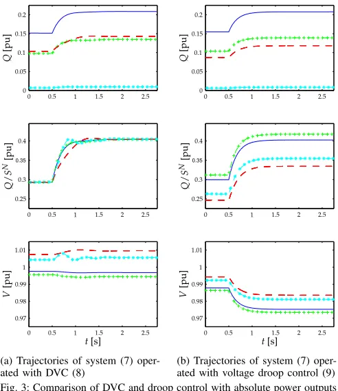
V. SIMULATION EXAMPLE
The performance of the proposed DVC (8) is now demon-strated and compared with the usual voltage droop control (9) via a simulation example based on the inner ring of the islanded Subnetwork 1 of the CIGRE benchmark MV distribution network [28]. In particular, we show the ability of the DVC (8) to quickly achieve a desired reactive power distribution after changes in the load.
The network consists of eight main buses and is shown in Fig. 2. We assume that the generation sources at buses 9b, 9c, 10b and 10c are operated with the DVC (8), re-spectively the droop control (9). The remaining sources are operated in PQ-mode. The distributed communication network is also depicted in Fig. 2. Note that the commu-nication is not all-to-all and that there is no central unit. The simulations are carried out in Plecs [29].
We associate to each inverter a power rating
SN = [0.517,0.353,0.333,0.023]pu, where pu denotes per unit values with respect to the base powerSbase= 3MVA.
For the DVC (8), we select a multiple of the nominal power rate of each source as weighting coefficient, i.e.χi= 5SiN,
i∼ N (cf. Remark 3.3) and, following Proposition 4.8, we setK=D.On the basis of selection criteria for frequency-active power droop [10], the parameters of the control (9) are set to Qd
i = 0.2SiN pu and kQi= 0.1/S N
i pu/pu. For both controls, we setVd
i = 1pu. To satisfy Assumption 4.5, the low pass filter time constants are set to τPi = 0.2 s,
i∼ N. The frequencies of the inverters are controlled with the usual frequency droop control, see e.g. [10], [11].
We consider the following scenario: at first, the system is operated under nominal loading conditions. Then, at
t= 0.5s, there is an increase in load at buses 3 and9.We compare the reactive power outputs and voltage trajectories of the inverters under the controls (8), respectively (9).
FC CHP FC CHP FC Bat PV PV PV PV PV PV PCC Main electrical network 110/20 kV 1 2 3 4 7 8 11 = = = = = = = = = = ∼ ∼ ∼ ∼ ∼ ∼ ∼ ∼ ∼ ∼ 9 9a 9b 9b 9c 9c 10 10a 10b 10b 10c 10c D is tr ib u te d co m m u n ic at io n n et w o rk E le ct ri ca l m ic ro g ri d
Fig. 2: 20 kV MV benchmark model adapted from [28] with eight main buses and generation sources of type: PV-Photovoltaic, FC-fuel cell, Bat-battery, CHP-CHP fuel cell. The symbol↓denotes a load and PCC denotes the point of common coupling to the main grid.
Moreover, compared to the droop control (9), the voltage levels remain close to the nominal value Vd = 1.
This becomes especially obvious from the voltage trajectories after the load step at t= 0.5 s, where all voltages are decreased under the droop control (9). Here, the DVC (8) merely causes small variations in the voltage amplitudes in order to satisfy the increased reactive power demand by the loads. This is an indication that no secondary voltage control may be necessary when operating the inverters with the DVC (8) – a clear advantage over the droop control (9).
Local stability under the control (8) is confirmed for both operating points via Proposition 4.8.
VI. CONCLUSION
We have proposed a consensus-based distributed voltage control (DVC), which solves the problem of reactive power sharing in inverter-based microgrids with inductive power lines. Unlike the widely used voltage droop control [1], [11], the DVC does guarantee a desired reactive power distribution in steady-state. Moreover, we have provided a necessary and sufficient condition for local exponential stability. The performance gain in terms of power sharing compared to the usual voltage droop control has been demonstrated in a simulation example. Future research will address the analysis of microgrids, in which the generation units are equipped with frequency droop control together with the DVC.
REFERENCES
[1] M. Chandorkar, D. Divan, and R. Adapa, “Control of parallel con-nected inverters in standalone AC supply systems,”IEEE Trans. on Industry Applications, vol. 29, no. 1, pp. 136 –143, jan/feb 1993. [2] R. Lasseter, “Microgrids,” inIEEE Power Engineering Society Winter
Meeting, 2002, vol. 1, 2002, pp. 305 – 308 vol.1.
[3] N. Hatziargyriou, H. Asano, R. Iravani, and C. Marnay, “Microgrids,” IEEE Pow. and Ener. Mag., vol. 5, no. 4, pp. 78 –94, july-aug. 2007. [4] H. Farhangi, “The path of the smart grid,”IEEE Power and Energy
Magazine, vol. 8, no. 1, pp. 18 –28, january-february 2010. [5] T. Green and M. Prodanovic, “Control of inverter-based micro-grids,”
Elec. Power Sys. Res., vol. Vol. 77, no. 9, pp. 1204–1213, july 2007. [6] P. Kundur,Power system stability and control. McGraw-Hill, 1994. [7] N. Pogaku, M. Prodanovic, and T. Green, “Modeling, analysis and testing of autonomous operation of an inverter-based microgrid,”IEEE Trans. on Power Electronics, vol. 22, no. 2, pp. 613 –625, march 2007. [8] J. W. Simpson-Porco, F. D¨orfler, and F. Bullo, “Synchronization and power sharing for droop-controlled inverters in islanded microgrids,” Automatica, vol. 49, no. 9, pp. 2603 – 2611, 2013.
[9] J. Schiffer, D. Goldin, J. Raisch, and T. Sezi, “Synchronization of droop-controlled microgrids with distributed rotational and electronic generation,” inProc. 52nd CDC, Florence, Italy, 2013.
[10] J. Schiffer, R. Ortega, A. Astolfi, J. Raisch, and T. Sezi, “Conditions for stability of droop–controlled inverter–based microgrids,” Automat-ica, 2014, accepted.
[11] J. Guerrero, P. Loh, M. Chandorkar, and T. Lee, “Advanced control architectures for intelligent microgrids – part I: Decentralized and hierarchical control,”IEEE Trans. on Industrial Electronics, vol. 60, no. 4, pp. 1254–1262, 2013.
0.35 Q / S N [p u ] Q [p u ] V [p u ] t[s] 0 0 0 0 1 1 1 1 2 2 2 1.5 1.5 1.5 2.5 2.5 2.5 0.05 0.98 0.97 0.1 0.2 0.3 0.4 0.5 0.5 0.5 0.15 0.25 1.01 0.99
(a) Trajectories of system (7) oper-ated with DVC (8)
0.35 Q / S N [p u ] Q [p u ] V [p u ] t[s] 0 0 0 0 1 1 1 1 2 2 2 1.5 1.5 1.5 2.5 2.5 2.5 0.05 0.1 0.2 0.3 0.4 0.5 0.5 0.5 0.15 0.25 1.01 0.99 0.98 0.97
(b) Trajectories of system (7) oper-ated with voltage droop control (9) Fig. 3: Comparison of DVC and droop control with absolute power outputs Qi in pu, power outputs relative to source ratingsQi/SiN and voltage
amplitudesViin pu corresponding to: FC CHP 9bi= 1’–’, FC CHP 9c i= 2’- -’, battery 10 bi= 3’- +’, FC 10ci= 4’-*’.
[12] Y. W. Li and C.-N. Kao, “An accurate power control strategy for power-electronics-interfaced distributed generation units operating in a low-voltage multibus microgrid,”IEEE Trans. on Power Electronics, vol. 24, no. 12, pp. 2977 –2988, dec. 2009.
[13] J. W. Simpson-Porco, F. D¨orfler, and F. Bullo, “Voltage stabilization in microgrids using quadratic droop control,” in Proc. 52nd CDC, Florence, Italy, 2013.
[14] C. K. Sao and P. W. Lehn, “Autonomous load sharing of voltage source converters,”IEEE Trans. on Power Delivery, vol. 20, no. 2, pp. 1009– 1016, 2005.
[15] Y. Mohamed and E. El-Saadany, “Adaptive decentralized droop con-troller to preserve power sharing stability of paralleled inverters in distributed generation microgrids,”IEEE Trans. on Power Electronics, vol. 23, no. 6, pp. 2806 –2816, nov. 2008.
[16] Q.-C. Zhong, “Robust droop controller for accurate proportional load sharing among inverters operated in parallel,”IEEE Trans. on Industrial Electronics, vol. 60, no. 4, pp. 1281–1290, 2013. [17] M. Marwali, J.-W. Jung, and A. Keyhani, “Control of distributed
generation systems - part ii: Load sharing control,”IEEE Trans. on Power Electronics, vol. 19, no. 6, pp. 1551 – 1561, nov. 2004. [18] A. Micallef, M. Apap, C. Spiteri-Staines, and J. M. Guerrero,
“Sec-ondary control for reactive power sharing in droop-controlled islanded microgrids,” inISIE. IEEE, 2012, pp. 1627–1633.
[19] Q. Shafiee, J. Guerrero, and J. Vasquez, “Distributed secondary control for islanded microgrids – a novel approach,”IEEE Trans. on Power Electronics, vol. 29, no. 2, pp. 1018–1031, 2014.
[20] R. A. Horn and C. R. Johnson,Matrix analysis. Cambridge university press, 2012.
[21] I. Sandberg and A. Willson Jr, “Some network-theoretic properties of nonlinear dc transistor networks,” Bell Syst. Tech. J, vol. 48, no. 5, pp. 1293–1311, 1969.
[22] C. Godsil and G. Royle,Algebraic Graph Theory. Springer, 2001. [23] J. Lopes, C. Moreira, and A. Madureira, “Defining control strategies
for microgrids islanded operation,” IEEE Trans. on Power Systems, vol. 21, no. 2, pp. 916 – 924, may 2006.
[24] J. Schiffer, A. Anta, T. D. Trung, J. Raisch, and T. Sezi, “On power sharing and stability in autonomous inverter-based microgrids,” in Proc. 51st CDC, Maui, HI, USA, 2012.
[25] R. Olfati-Saber, J. A. Fax, and R. M. Murray, “Consensus and cooperation in networked multi-agent systems,” Proceedings of the IEEE, vol. 95, no. 1, pp. 215–233, 2007.
[26] S. Rabinowitz, “How to find the square root of a complex number,” Mathematics and Informatics Quarterly, vol. 3, pp. 54–56, 1993. [27] H. K. Khalil,Nonlinear systems. Prentice Hall, 2002, vol. 3. [28] K. Rudion, A. Orths, Z. Styczynski, and K. Strunz, “Design of
benchmark of medium voltage distribution network for investigation of DG integration,” inIEEE PESGM, 2006.
[image:8.612.54.297.55.161.2]