Applying Data Analytics to Improve Multi-Asset Portfolio Performance

Theses Thesis/Dissertation Collections

6-2017

Applying Data Analytics to Improve Multi-Asset

Portfolio Performance

Amrith Akula

[email protected]

Follow this and additional works at:http://scholarworks.rit.edu/theses

This Thesis is brought to you for free and open access by the Thesis/Dissertation Collections at RIT Scholar Works. It has been accepted for inclusion in Theses by an authorized administrator of RIT Scholar Works. For more information, please [email protected].

Recommended Citation

Multi-Asset Portfolio Performance

by

Amrith Akula

A Thesis Submitted

in

Partial Fulfillment of the

Requirements for the Degree of

Master of Science

in

Computer Science

Supervised by

Dr. Rajendra Raj

Department of Computer Science

B. Thomas Golisano College of Computing and Information Sciences

Rochester Institute of Technology

Rochester, New York

The thesis “Applying Data Analytics to Improve Multi-Asset Portfolio Performance” by

Amrith Akula has been examined and approved by the following Examination Committee:

Dr. Rajendra Raj Professor

Thesis Committee Chair

Dr. Leonid Reznik Professor

Thesis Committee Reader

Dr. Carol Romanowski Professor

Dedication

To my parents Ravi and Viji, for their unwavering support through my education and

ultimately in the completion of my Master’s degree.

And to Dr. Raj, for having the highest level of patience to guide me through a Master’s

Abstract

Applying Data Analytics to Improve Multi-Asset Portfolio

Performance

Amrith Akula

Supervising Professor: Dr. Rajendra Raj

The number of casual investors allocating funds into financial exchanges has surged due

to the increased availability of trading accounts on multiple platforms. These investors

quite often invest only in one type of asset, stocks. Stocks are known to experience sudden

market shifts and extreme volatility based on factors that the investors may not be able to

control. Existing applications of data mining stocks perform well, but if the entire stock

market performs poorly, investors can face severe losses. This study utilized a data

min-ing tool that evaluates two other classes of investments: the commodities market and the

currency exchange market. Three avenues of data mining were implemented as solutions,

a neural network, logistic regression and a decision tree, to classify the buying and selling

of investments. The results presented that unless in a bullish market scenario, utilizing a

multi-asset portfolio with backed by a data mining tool can prove beneficial to an investor.

In a bearish market, this study outlined how the performance of the multi-asset portfolio is

drastically better than investing using a standalone stock classifier or investing in an index

tracked product. In a volatile market, results showed that a multi-asset portfolio is

compet-itive with a standalone stock classifier and in many scenarios even out performed. Overall,

Contents

Dedication. . . iii

Abstract . . . iv

1 Introduction. . . 1

1.1 Background . . . 3

1.1.1 Stocks and Data Mining . . . 3

1.1.2 Artificial Neural Networks . . . 4

1.1.3 Logistic Regression . . . 5

1.1.4 Decision Tree . . . 6

1.2 Problem Statement . . . 7

1.3 Related Work . . . 7

1.4 Hypothesis . . . 9

1.4.1 Initial Portfolio Distribution Consideration . . . 10

1.4.2 Gain Threshold . . . 10

1.5 Roadmap . . . 11

2 Design and Implementation . . . 12

2.1 Design . . . 12

2.1.1 Application Design . . . 12

2.2 Implementation . . . 16

2.3 Testing . . . 17

3 Analysis . . . 18

3.1 Analysis Methodology . . . 18

3.2 Environment . . . 19

3.3 One Asset Type Distribution . . . 19

3.3.1 Bull Market . . . 19

3.3.3 Volatile Market . . . 25

3.4 Equal Distribution in Three Assets . . . 29

3.4.1 Review . . . 31

4 Conclusions . . . 33

4.1 Current Status . . . 33

4.2 Future Work . . . 34

4.3 Lessons Learned . . . 35

List of Tables

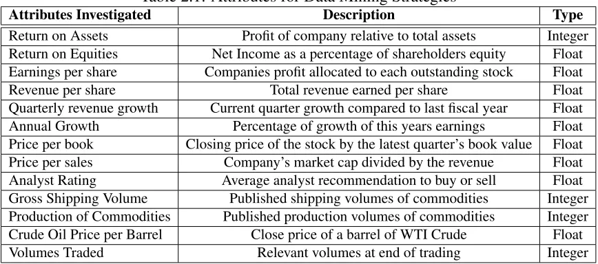
2.1 Attributes for Data Mining Strategies . . . 17

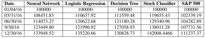
3.1 Portfolio Values in Bull Market per Quarter 2016 . . . 21

3.2 Confusion Matrix for Decision Tree in Bull Market . . . 22

3.3 Confusion Matrix for Neural Network in Bull Market . . . 22

3.4 Confusion Matrix for Logistic Regression in Bull Market . . . 22

3.5 Portfolio Values in Bear Market per Quarter 2008 . . . 24

3.6 Confusion Matrix for Neural Network in Bear Market . . . 25

3.7 Confusion Matrix for Logistic Regression in Bear Market . . . 25

3.8 Confusion Matrix for Decision Tree in Bear Market . . . 26

3.9 Portfolio Values in Bear Market per Quarter 2008 . . . 27

3.10 Confusion Matrix for Neural Network in Volatile Market . . . 28

3.11 Confusion Matrix for Logistic Regression in Volatile Market . . . 29

3.12 Confusion Matrix for Decision Tree in Volatile Market . . . 29

3.13 Portfolio Values in Volatile Market per Quarter 2015 with Split Initial Dis-tribution . . . 31

3.14 Performance Evaluation for Stock Level Classifier . . . 31

3.15 Performance Evaluation for Commodity Level Classifier . . . 32

List of Figures

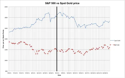
1.1 The change in price per ounce of gold and basis points of the S&P 500 be-tween July 8th2011 and November 2nd2011. Between July 8thand Septem-ber 2nd, gold prices increased while the S&P 500 Index fell. In the next two months gold prices fell 6.63% while the S&P 500 Index rose 5.45%. . . 2 1.2 This graph displays the closing price of the YUM company stock between

26th _{August 2015 and 26}th _{August 2016. On this graph, based on the 10%}

gain and 5% loss strategy, key data points have been identified, where red indicates sell and green indicates the buy classification. . . 11

2.1 This workflow represents the day to day evaluation of the portfolio and the application of the two stage data mining tool to pick investment choices. . . 14

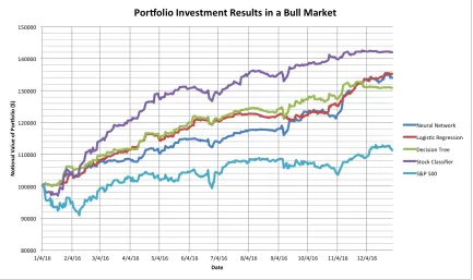
3.1 This graph displays the resulting portfolio value change over the fiscal year 2016. The results of investments based on the three classification tech-niques are presented with a stock market focused investment tool and the S & P 500 Index for comparison. . . 20 3.2 This figure presents the resulting portfolio value change over the fiscal year

2008. The results of investments based on the three classification tech-niques are presented with a stock market focused investment tool and the S & P 500 Index for comparison. . . 23 3.3 This figure presents the resulting portfolio value change over the fiscal year

2015. The change in value of the assets identified by the three classification techniques are presented with a stock market focused investment tool and the S & P 500 Index for comparison. . . 26 3.4 This figure presents the resulting portfolio value change over the fiscal year

Chapter 1

Introduction

In recent years, many secure financial applications have been developed for the end user,

lowering barriers between the potential investors and financial exchanges. Bank of

Amer-ica recently noted that mobile stock trading went up 200% year over year between 2012 and

2013, and mobile trading now accounts to be between 10% to 20% of its total trading

vol-ume [5]. MarketWatch explains that this trend is not isolated to banks but is also prevalent

in all major providers of equity trading [5]. As a result, many new or casual investors may

not be aware of sudden market shifts, trends in the market, or they may be distracted by

other facets of life. I plan to create a portfolio maintenance mechanism that allows for users

to diversify their investments from just stocks, into commodities and bonds through the use

of futures contracts. Using data-mining techniques, we can inform these end users about

when to reconsider their investments in one particular asset class and shift it to another.

Example 1: Consider that a similar recession like scenario is reached where consumers

are afraid to spend money and insist on saving. This causes weak demand for products,

which in turn curtails the sales of the companies making the products causing investors in

these companies to panic. In such a situation, we can see that many investors diversify their

investments into other stable products such as commodities - which include gold, silver,

crude oil and other staples. Investors also choose to invest in bonds such as the United

States Treasury Bond, which provides them interest over year in the form of coupons.

In our example if the S&P 500 index is observed between July 8th_{2011, and the index’s}

basis points on September 2nd2011 is compared, we can see a change of -12.6%. The S&P

period investigating spot gold prices per ounce reveals a change 21.5%. Ideally, if market

forces could have been predicted, and an investor could have shifted their investments into

commodities like gold, Figure 1 represents the change in price and points over this time

period. Now if we shift the time period to September 2nd_{2011 to November 2}nd_{2011, spot}

gold prices reduced from $1854 per ounce to $1731 per ounce, a change of -6.63%. At

the same time however the S&P 500 Index rose from 1173.91 basis points to 1237.90 basis

points, an increase of 5.45%. In this scenario, it would have been highly advantageous for

an investor to shift their investments from being heavy on the gold and other commodities

to stocks and other equities resulting in a tidy profit.

Figure 1.1: The change in price per ounce of gold and basis points of the S&P 500 between July 8th _{2011 and November 2}nd _{2011. Between July 8}th _{and September 2}nd_{, gold prices}

increased while the S&P 500 Index fell. In the next two months gold prices fell 6.63% while the S&P 500 Index rose 5.45%.

If we look at the data for stocks and futures, we can get information from a significant

time period, and down to fine grade time slices. Studies such as Haregreaves et al. have

of adding more choices to the same portfolio such as commodities and currencies. When

investing in futures, buying and selling the position are represented as contracts that can be

called or put. By purchasing the option on calling, the investor has the right to purchase

the underlying security at the stated price. If the prevailing market price of the security

is greater than the price of the contract, the investor is ”in the money” and can liquidate

his position for a profit. In the currency market, major markets include the trading of

international currencies with the U.S. Dollar. As this study utilizes the U.S. Dollar as the

base currency for investment, if the reciprocal foreign currency gains in value, an investor

owning the foreign currency would have a bigger position if they were to liquidate back

to U.S. Dollars. As each of these different asset types have unique economic and market

factors that affect the performance, it will be vital to identify those factors into quantifiable

attributes. By utilizing those attributes with reference to the market price, one can create

a data mining tool to identify the opportune time to buy and sell a position in the given

market. The remainder of this introduction focuses on describing the data mining tools

utilized to a success in past studies and creating a strategy to invest and proactively maintain

a portfolio.

1.1

Background

1.1.1

Stocks and Data Mining

By investigating stock prices over a large period of time coupled with large attribute sets,

researchers have utilized techniques such as neural networks and logistic regression to

iden-tify opportunities to purchase and sell stocks where underlying trends are observed and

market changes can be predicted[6]. Data mining allows end users to make sense of the

data, and as stock prices and economic factors are routinely recorded they test the abilities

of data mining techniques in a real world environment. The real strength in data mining

stock data is that due to its periodical nature and the ability to classify stocks either as a

1.1.2

Artificial Neural Networks

An artificial neural network operates on the divide and conquer paradigm[7]. They emulate

biological neural systems by representing the network as massively parallel process that

involve processing elements connected together. This representation starts by receiving

inputs analogous to electrochemical impulses as xi. Next these inputs are multiplied by

weights, which represent the strength of these input signals, wij. This helps compute the

activation of a neuron, wherein once the summation of these inputs and weights surpass a

certain threshold, an output is triggered. Overall we can represent the equation as Uj =

Σ(Xi ·Wij)[10].

Backpropagation and learning are features of neural networks currently in use in many

studies[2]. A new layer, the hidden layer, is placed between the input and output layers

where all input nodes connect to each of the hidden layer nodes and all the hidden layer

nodes connect to the output nodes, but not to any nodes in the same layer. By utilizing

one or more hidden layers, the weights in the network will be updated to prevent loss. A

multilayer neural network escapes the linear limitation of a single layer network and allows

internal classification rules to be created where features can be learnt in each layer[8]. We

can further this learning by training the network, this is done by determining the error,

a difference between the desired response and the actual response. By propagating this

error backward through the network, we can further adjust the weights of the neurons to

minimize the error of the network for the same outputs.

In the stock data mining studies, the attributes attached to the stock are deemed the

weights and the output is traditionally the outcome the researcher desires: buy, sell or

hold. By sequentially training the neural network with data we can train the network to

optimize the weights and establish patterns to which our classification occurs. Over time

the total error will become smaller and after we set a specified threshold we can begin

testing the neural network on data used in the training to test the validity of the training.

In terms of stocks and futures classification, the assets neural networks posses include the

backpropagation and learning - as market trends change so can the neural network, thus

adapting to newer trends. Lastly, by assigning and altering weights to the inputs and the

hidden layers, we can interpret what variables to investigate when looking at past data.

1.1.3

Logistic Regression

To classify the stocks and futures into buy, sell and hold a multinomal logistic regression

classifier can be used. This classifier uses a combination of binary logistic regressions

which are traditionally a binary classifier. In this scenario the classifier will compare buy

and not buy, sell and not sell and hold and not hold. Thus performing two comparisons for

each of our independent variables. The logistic regression model works on the reasoning

that the probability of a systemSpcorresponding to a certain inputxpresults in the system’s

outputyq. This is modeled as equation 1.

P(yq/Sp, xq) (1.1)

Logistic regression uses the sigmoid function to aid in the learning of classification of

data points by employing multiple regression coefficients. This model can be represented

as equation 2.

P(y= 1) = 1

1 +e−(β0+β1x1+β2x2...+βpxp) (1.2) Equation 1 represents the probability of our event, in this paper either a buy, a sell or a hold.

β represents the regression coefficients that are applied to linear models x that represent

patterns in the data[4]. Using this model, we can predict a discrete outcome, such as group

membership, from a set of variables that may be continuous, discrete, dichotomous, or a

combination of these. When we apply this scenario to stock and future data, we can take

into account a series of attributes upon which this classifier can be built[1].

When considering the application of logistic regression as a classifier, one of the major

advantages is that it is noise insensitive and avoids overfitting to the training data. While

not in use in this study, logistic regression can be utilized in a distributed setup, where the

of picking best performing investment options, logistic regression provides a probability of

classification which can be used in this scenario[1]. By using the probability as a rank,

logistic regression provides an alternative tool to pick investment options in a scenario

where multiple options exist.

1.1.4

Decision Tree

In the field of data mining and its application of identifying stocks, decision trees are used

in several studies to positive effect[2]. They can be used to represent both classifiers and

regression models, while offering a hierarchical model of decisions. They are particularly

useful when investigating the relationship between large number of attributes and the target

variable.

A C5.0 decision tree has been used successfully by Hargreaves et. al in their study

investigating stocks in the Australian stock market. A decision tree itself is composed

of its training data set of S = s1, s2, ..., si.This series represents a set of data which has

been already classified. Each data point is further broken down into a vector composed of

attributes represented as (x1,i, x2,i, ..., xp,i). The attributes xalso include the class which

the setsi falls into. The decision tree then starts to create decision points between classes

based on each attribute which most effectively splits the data into one or more of the classes

based on information gained from the entropy of a data set. Entropy is represented as the

equation 3.

Entropy=X

i

−pilog2pi (1.3)

Entropy is measured as the probability p of class i in the data set. Information gain is

calculated by looking at the entropy of the children and comparing that to the entropy of

the parent. This is represented as equation 4.

Inf ormationGain =Entropy(P arent)−AverageEntropy(Children) (1.4)

Once the attribute with the most information gain has been identified, it will be used as the

An advantage of decision trees is that the rules that are derived can be easily interpreted and

applied to queries for manual selection. The rule definition is easily interpreted and can be

applied on the data set. The disadvantage of having these rules defined and of decision trees

in general is that learning is not supported as well as neural networks and as a result the

weights of each of the attributes will not be changed unless the tree is retrained. This may

not be a problem in a stock and futures situation where markets operate between 9:30am

and 4pm, but over time the training the decision tree with more data points will take more

time.

1.2

Problem Statement

The aim of the proposed work in this thesis is the investigation and development of a

multi-asset based investment classifier backed by data mining. Each classification technique has

been described with how the information gained from the attributes will build towards

over-coming existing limitations of investing in stocks singularly. By adding varied investment

choices, the correlating attributes will be key to mitigate loses in the event that the entire

economy performs poorly. The goal of this project is to reflect an investor’s portfolio and

replicate investment decisions as they would occur in the market and utilize the strength of

the information stored in the classifiers to make rewarding investment choices.

1.3

Related Work

There is concerted effort in the field of computer science to use data mining techniques to

pick stocks, whereas futures are often overlooked. Muh-Cherng et. al applied a decision

tree based classifier to pick stocks in the Taiwan and NASDAQ stock exchanges. In their

study, the comparison uses a classifier to a selling or buying stocks when they surpass a

certain price threshold. In their study, they also utilize CPI(consumer price index) as one of

the attributes to represent the inflation rate, which has been known to have an effect on stock

return (ACARR), which calculates the return made on investment taking into consideration

trading taxes and fees in addition to the actual performance of the stock. This metric can

be useful for portfolios that range for more than one year[11].

Hargreaves et. al present a study that investigates both decision trees as well as a neural

network. Their paper presents several concepts that will be useful to build upon. Both

Muh-Cherng et. al and Hargreaves et. al limit the scope of the market in their papers

to one field. By choosing a sector in the stock market, we can limit the data preparation

required aggregating economic and historical data. For example, there are 1033 companies

listed in the financial sector in NASDAQ, NYSE and AMEX exchanges. Hargreaves et.

al however utilize this sector selection as the first point in the stock picking process[3].

They investigated each of the sectors and selected the sector that performed the best over 3

months prior to the period they were performing the tests. When selecting futures based on

commodities contracts, there is some variation based on the contract size and the exchange

which this commodity is traded on, however the best performing futures will be picked

using the classifiers rather than selecting an sector.

Another interesting correlation between both Muh-Cherng et. al and Hargreaves et. al

is that they utilized some form of trading strategy to determine when to buy and when to

sell their positions. Hargreaves et. al use a 10% gain as an exit strategy. This infers that

assuming that a stock grows more than 10% over the period that the portfolio is holding

this script, the portfolio then executes a sell on all the shares for that particular script.

Conversely, a 5% loss was utilized as an exit strategy to liquidate positions held which

resulted in losses. This ensures that even with unpredictable swings in the market, the

investor can exit their positions and use the data mining tools to re-invest their capital.

Hargreaves et. al also utilize some useful attributes in their classifiers, these attributes

will be key to ensuring the success of the stock classifiers. Some attributes include return

on equity, return on assets, earnings per share, revenue per share, and quarterly revenue

growth. When it comes to the futures, there are fewer attributes that indicate when it comes

production, unemployment rate and oil rig data that are available through public databases.

These attributes can be evaluated by using the random forest model. This model produces

a score that represents the link between the attribute and the output hence ensuring that

appropriate attributes are chosen for the classifiers[3].

1.4

Hypothesis

Current studies have investigated using stocks and implementing data mining solutions to

adequate success, however this is not enough in the situation where the entire economy does

poorly or if other avenues of investment such as currency or commodity futures present

themselves. Hence, to take into consideration these other avenues of investment, a solution

must be probed where in economic factors are coupled with data mining tools that take into

account new economic trends.

The hypothesis underlying this study is that a two stage data mining solution would

help allocate capital into varied investments by utilizing classification, neural networks and

logistic regression in a manner that utilizes their classification abilities in more avenues. As

the result of this expanded investment choice, one would expect greater growth of a

port-folio over a similar period of investment. The hypothesis can be validated by investigating

three periods in the market: a growing market, a declining market and a volatile market.

In each scenario, by classifying the best available options to invest and utilizing a second

classification to identify which market to invest in, this solution should provide the best

investment scenario.

To further evaluate the hypothesis, the performance of the multi-asset portfolio will be

compared to a portfolio that only utilized data mining for investing in stocks only. The

performance will also be compared to an index based investment strategy, investing in the

S&P 500 index and the underlying stocks. By training the classifiers with a dataset that

includes a large history, multiple scenarios can be trained into the data mining algorithms

1.4.1

Initial Portfolio Distribution Consideration

As this study proposes a novel solution to the security investment problem where the funds

can be split into the asset types, the initial split into each asset class may impact the

per-formance of the portfolio. As a result, it is worth investigating four basic scenarios of how

these funds are distributed. In the first scenario, the funds should be split evenly between

the stocks, currencies and commodities. This split will create a diversified portfolio that

should be prone to less risk, but at the same time it may compromise the gain achievable

by investing more in one type of asset. The other three scenarios would involve investing

predominantly in one of the three asset classes. These three scenarios would rely on the

data mining algorithm to determine the most opportune time to re-evaluate the market

con-ditions and appropriately reinvest into a different asset type. An additional benefit of this

strategy is that by exposing more risk by investing in one asset type, a greater profit is also

possible.

1.4.2

Gain Threshold

Another major factor in this study is the investment strategy that identifies when to close

the existing position. As mentioned, existing studies that have mined stocks have used a

strategy of 10% gain and 5% loss as entry and exit strategies respectively[3]. However,

as currencies and commodities have not been investigated in a similar manner, this study

will also investigate the appropriate trading strategy. By investigating a range of values at

which this strategy is used, we can determine the most effective trading strategy. In figure

2, data points where trends change between a buy and sell set by the 10% gain and 5% loss

threshold have been identified. It will be key to identify similar points across all available

Figure 1.2: This graph displays the closing price of the YUM company stock between 26th August 2015 and 26th _{August 2016. On this graph, based on the 10% gain and 5% loss}

strategy, key data points have been identified, where red indicates sell and green indicates the buy classification.

1.5

Roadmap

The remainder of this report is dedicated to the detailed implementation and analysis of the

results obtained from utilizing the multi-asset classifier. Design and implementation

infor-mation are described in section 2. Section 3 contains the results and testing methodologies.

Chapter 2

Design and Implementation

2.1

Design

To investigate the performance of a multi-asset based classifier, the project focused on

the recreation of an investment situation by creating datasets that is available to common

investors. This allows for day by day application of investment decisions based on the

two level classifier that has been created. At each of the two levels, the data output from

the classifier and appropriately equating the investment choices in dollar value is key to

the successful implementation and verification of the declared hypothesis. The application

maintaining the portfolio is designed to maintain the investment choices and accurately

aggregating the portfolio’s value based on the day value of the actual investment choice.

The same application is also used to evaluate the performance of the single asset type

portfolio’s performance for comparison.

2.1.1

Application Design

The application design involves primarily in a Java application that maintains the user’s

state on a daily basis. This state will be altered on a daily basis based on the choices

made by the data mining sub-algorithms. These data mining algorithms will be created and

maintained using an implementation of the R statistical programming language. R provides

a configurable environment into which the training data can be loaded as a .csv file. The

java program will handle the decisions created as a result of the data mining tools and

data mining algorithms. For each asset type, the subset of securities closing price per day

data will be acquired for a common 8 year period that includes all three market scenarios

bull, bear, volatile. Other attributes are also applied to each of days where available. Once

the data is compiled, data warehousing techniques will be used to identify missing data and

evaluate the best possible action to remedy the data. For each of the security available to

invest, a simple evaluation of the closing price is conducted for training the classifier on

when to buy and when to sell as the base classification. Similarly, a classification must be

made on the picking which of the asset type to invest in based on an index value. Finally,

when the algorithm is ready to test, each day’s closing price is added to the data mining

tool to evaluate the actions that should be performed at each given day. As the actions are

performed, the investment choices are updated with the new profit or loss and restated.

Another aspect of the solution is the application of attributes to aid the data mining

process and discover statistically significant trends in the data which may be used to the

create decisions. One key principle of this study is that by broadening the scope of the

assets available to invest in, the risk is equally mitigated. Hence to ensure that similar

data mining techniques can be applied to the new assets, attributes that relate to the price

and environment of currency and commodity investment choices are presented in Table 1.

In addition to attributes proven to provide success in mining stocks, economic attributes

are included in Table 1. Using methods such as the random forest model suggested by

Hargreaves et. al[3], and accuracy tests on trained classifiers the following attributes were

utilized in the study.

The day to day management of the portfolio’s assets is illustrated in Figure 3. In this

study, a top level decision is made to identify which of the three asset classes best suits the

current market and economic conditions. After identifying the market market to invest in, a

lower level data miner evaluates the available securities and identifies the product with best

gain potential based on learnt data. The lower level classifiers have been illustrated with the

sample exit strategies based of the original acquisition price, where a profit of 10% results

loss. The last exit strategy is when stagnation occurs, if an investment remains inside the

+10% and -5% threshold for over 30 days, the position will be liquidated on the 30th day.

Figure 2.1: This workflow represents the day to day evaluation of the portfolio and the application of the two stage data mining tool to pick investment choices.

To streamline of the implementation and validation of the hypothesis, the following

assumptions are required.

• The data investigated will be utilized as a numeric type and similarly data such as

analyst ratings will be similarly converted to maintain consistency.

• All data will be presented as closely as possible to a daily basis, matching the price

of security, present as an end of day value.

• An average profit and loss exit strategy will be applied across each asset type to

• The data presented will be evaluated using open refine to identify anomalies and

clean data.

• Holidays across the markets will be normalized by excluding that particular day from

the data.

• A constant exchange rate and end of day values will be maintained to calculate the

current portfolios value.

• The time period of the investigation will range for 1 year, loading these data points

into the algorithm for learning where applicable.

• A visualization of the portfolio’s performance will be provided, a comparison

be-tween the portfolio and popular indices will be available.

• The same data provided to the multi-asset classifier will be provided to the stock

classifier for an easier comparison.

• The stocks in the Dow Jones Industrial Average will be used as the core stock

invest-ment option, reflecting multiple large, popular and diverse companies not limited to

a single industry.

• Investments held after 30 days but still inside 10% gain and 5% loss threshold will be liquidated.

• Each investment block will be $10,000 totaling a sum of $100,000 at the start of each scenario.

2.2

Implementation

The implementation of the multi-asset classifier was guided by the design scheme and

em-ployed the trading strategy as the basis for the creation of Java application. This application

was created in the Java SE 6.0 environment, relying on CSV data generated by the

clas-sifiers trained in R version 3.2.4. Within R, the neuralnet package was used to train then

neural network based classifier, the nnet package was used to train the logistic regression

based and lastly the ctree package was used to train the decision tree classifier. Additionally

Python 2.7.4 was utilized with the Yahoo Finance API to allow for the retrieval of financial

data used to train the classification tools. Lastly, OpenRefine 2.6 was utilized to normalize

the data utilized in this project.

During the initial creation of the training data, it was observed that a significant set

can be obtained from Yahoo Finance. As a result, the Yahoo Finance API was utilized in

Python to generate custom CSV files containing the appropriate data sets. After analyzing

the patterns in historical data, the training set was created with a range from January 1,

1999 to December 31 2007. As discussed previously this training set encompasses the bull,

bear and volatile market appropriate for holistically validating the hypothesis. To test the

trained classifiers, 2008 is utilized as the bear market data set, 2016 was utilized as the bull

market data set and 2015 was utilized as the volatile market.

Additional observations indicated that the stock data set contained the most exchange

holidays. Considering that this data set is the key indicator, OpenRefine was utilized to

create a normalized dataset per asset for the 8 year training period. During the creation

of the R based classifiers it became apparent that utilizing the Java based libraries would

become cumbersome, and instead the CSV output from the classifiers was used as an input

in the Java Application instead. Similarly, the output of the Java application was utilized

in the individual asset classifiers to test the model. Additionally, the neural network and

logistic regression classifiers provided output indicating the probability of classification

into buy or sell. The decision tree classifier however, would rather classify the test data into

Table 2.1: Attributes for Data Mining Strategies

Attributes Investigated Description Type

Return on Assets Profit of company relative to total assets Integer

Return on Equities Net Income as a percentage of shareholders equity Float Earnings per share Companies profit allocated to each outstanding stock Float

Revenue per share Total revenue earned per share Float

Quarterly revenue growth Current quarter growth compared to last fiscal year Float

Annual Growth Percentage of growth of this years earnings Float

Price per book Closing price of the stock by the latest quarter’s book value Float

Price per sales Company’s market cap divided by the revenue Float

Analyst Rating Average analyst recommendation to buy or sell Float

Gross Shipping Volume Published shipping volumes of commodities Integer Production of Commodities Published production volumes of commodities Integer Crude Oil Price per Barrel Close price of a barrel of WTI Crude Float

Volumes Traded Relevant volumes at end of trading Integer

testing the same set 10 times was used as a decider.

2.3

Testing

Four major components were developed for the validation of this projects hypothesis. First

the datasets would be created using the python utilizing the end of day recorded values

populating the attributes described in Table 2.1. This dataset allows for the appropriate

information gain used in the creation and testing of classifiers. To train the asset type

classification, the training dataset based on the S & P 500 Index and custom currency and

commodities index. These two indexes were weighted by the volume, creating a buffered

Chapter 3

Analysis

3.1

Analysis Methodology

The approach to testing, analysis and evaluation of the results of this project is focused

on investigating the performance of each of the classifiers both by exploring the monetary

results of the portfolio and by statistically evaluating the results of the classifiers to known

values. Testing has been split first into two major branches, dividing the testing between

the initial distribution investment into One Asset Type and Equally Split Between All Asset

Types. In the One Asset Type section, the testing is further split into the three scenarios

of bull, bear and volatile market. In the testing scenario where the initial distribution is

split between all three asset classes validates its results in a volatile market scenario.

Ad-ditionally these four scenarios are compared to a benchmark performance of a singular

stock classifier, utilizing stocks as its only investment option. Another benchmark is the

S&P 500, a flat investment at the start of the year is also utilized as a metric. It is key to

identify the different investment choices observed within each individual market scenario

and observe the trajectory of the portfolio’s value. Success within each individual test

sce-nario in relation to the stated hypothesis would reflect a higher portfolio balance at the end

of the year, additionally confusion matrices can be employed to test the efficacy of each

individual classification technique, with the more precise classifier performing the best.

The remainder of this section focuses on results and discussion of each the individual test

3.2

Environment

Project implementation and all testing has been performed on an Apple MacBook Pro,

utilizing an Intel Core i7 2.3GHz processor and 8GB of system memory. While future

performance of the portfolio should remain independent of the machine, the training time

for each classification model would be dependent on the host machine capabilities.

3.3

One Asset Type Distribution

The first test scenario describes a new investor scenario as the first day in each test

sce-nario will have a singular asset type classification. To test this scesce-nario, an investment

of $100,000 was divided into ten investment blocks and subsequently tested into the

ap-propriate asset level classifier. Each initial investment block will remain consistent across

the three market scenarios and the reciprocal gain or loss will be reinvested based on the

classification. The three market scenarios are designed to test multiple economic forces

influencing the asset prices and ensure that no unintentional bias or bell-weather pattern is

introduced into the training set.

3.3.1

Bull Market

This test scenario representing fiscal year 2016 is indicative of the economy doing well and

similarly reflecting in the stock market’s performance as well. Ideally the gains of the stock

market showcase the performance of the economy and produce the most gains, however in

the testing observed the initial investment type is in the currencies asset class. Figure 3.1

tracks the investment performance for 2016, comparing the results to a standalone stock

classifier and the S&P 500 Index.

From the results it is observable that the standalone stock classifier performed had the

best end performance by ending with the portfolio with the highest asset value. When

comparing the returns, the standalone classifier produced returns of nearly 42%. The

Figure 3.1: This graph displays the resulting portfolio value change over the fiscal year 2016. The results of investments based on the three classification techniques are presented with a stock market focused investment tool and the S & P 500 Index for comparison.

of 35.2% and lastly the decision tree produced a return of 30.8%. A quarterly breakdown of

each tool investigated is highlighted in Table 3.1. First and foremost, all data mining

tech-niques performed better than the S&P500 Index, which returned a gain of 11.1%, indicating

that the training data set and the economic factors were able to add useful information gain

to assist an investor.

To analyze further, one of the interesting results is the underperformance of the Decision

Tree, considering that it uses the same classification technique as the standalone stock

classifier, it produced a return of nearly 11.2% less that the stand alone stock classifier.

Using Figure 3.1 we can see that while the Decision Tree had a stronger initial month

than stand alone stock classifier, the performance slowly starts to widen. Another point to

notice in Figure 3.1 is that although the Neural Network and the Logistic Regression based

portfolios had a strong December, the Decision Tree portfolio starts to flatline. This pattern

Table 3.1: Portfolio Values in Bull Market per Quarter 2016

Date Neural Network Logistic Regression Decision Tree Stock Classifier S&P 500

01/04/16 100000 100000 100000 100000 100000 03/31/16 108451.83 110637.92 111559.48 119655.43 102339.19 06/30/16 114073.27 120622.68 121180.28 129340.96 104282.89 9/30/16 123449.80 121996.92 127058.93 138011.28 107731.56 12/30/16 133948.52 135220.66 130828.73 142008.4466 111237.37

Digging deeper, utilizing the output from the Java application to see the raw investment

choices, it is observable that the decision tree missed out on investing in the USD / Yen

currency exchange. This one asset appreciated nearly 16.2% between October and its peak

in December. Investigating the overall classification performance of the Decision Tree, we

can see that the True Positives indicate the actual predicted classification which corresponds

to an actual classification. In Table 3.2, we can see that the Decision Tree has 15 True

Positives, dividing the True Positives by the sum of True Positives and False Positives we

arrive at the Precision for this classification. In this scenario the Precision for Currency

Investments by the Decision Tree stands at 55.6%. This strongly provides a reason why the

USD / Yen currency investment choice was not utilized by the Decision Tree.

The specificity of the Decision Tree for Currency is calculated by dividing the True

Negatives by the Sum of True Negatives and False Positives. In this scenario, there are 218

True Negatives and 12 False Positives. This results in a specificity of 94.8%, indicating

that the decision tree will rarely register a false positive that is not the target for testing.

Considering that in the bull market example where stocks were shown to represent majority

of the economic benefits, being highly specific for investing in the currency market which

had the fewest individual gains does have some meaningful result.

The Decision Tree had a stronger performance in the Commodities investment category.

From Table 3.2, the True Positives for Commodities was at 61.8%, and the True Positive

rate for stocks was at 89.3%, which is definitely helpful in a bull market. Looking at

data in Table 3.3 and 3.4, the Neural Network and the Logistic Regression tools produce a

Table 3.2: Confusion Matrix for Decision Tree in Bull Market

the lack of overall attempts to test the classification of investment in Currency Exchange,

a lower True Positive can be observed. Additionally, a specificity of 97% and 95.7% is

calculated based on the results obtained from the Neural Network and Logistic Regression

tools respectively.

Table 3.3: Confusion Matrix for Neural Network in Bull Market

Table 3.4: Confusion Matrix for Logistic Regression in Bull Market

3.3.2

Bear Market

A bear market represents the economy doing poorly, and this is reflected by the stock

a significant degradation of the market value over the fiscal year. The year 2008 exhibits

some unique characteristics, there is an initial dip of more than 10% within the first three

months, however by June of 2008 these losses are pared. The stock market in the second

half of the year significantly responds to the financial uncertainties and loses nearly 48.1%

by November 20th. Figure 3.2 presents these market conditions by plotting the S & P 500

Index and compares the performance of the data mining algorithms in 2008.

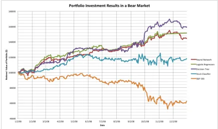
Figure 3.2: This figure presents the resulting portfolio value change over the fiscal year 2008. The results of investments based on the three classification techniques are presented with a stock market focused investment tool and the S & P 500 Index for comparison.

The results infer that due to the major financial crisis the stock market performed

ex-tremely poorly, an investor with capital invested in a fund tracking the S & P 500 Index

would have lost 37.6% of the value over the course of 2008. With that being said, the stand

alone stock classifier produced a return of 11.8% over the same period. This indicates that

despite the market tumbling, certain stocks were still able to appreciate in value. The neural

network tool produced a return of 44.5%, the logistic regression tool produced a return of

each tool investigated is highlighted in Table 3.5.

Looking at the results, the multi-asset based classification tools performed significantly

better than the stand alone stock classifier and they completely out performed the S & P

500 Index. Using Figure 3.2, it is observable that all three multi-asset algorithms start to

appreciate in value significantly after October 2nd. Looking at the underlying investment

choice, all three algorithms shifted investments from stocks to currencies during the month

of June. Currencies such as the Korean Won and Mexican Peso increased appreciated in

values of roughly 44% and 34% respectively using June 1st_{2008 as a base value date. This}

point is most observable in the performance of the decision tree classifier, although this

portfolio was lagging behind the other two tools as of June 6st_{, aggressive investments into}

the Currency Exchange market ultimately yielded with the best performing portfolio.

Table 3.5: Portfolio Values in Bear Market per Quarter 2008

Date Neural Network Logistic Regression Decision Tree Stock Classifier S&P 500

01/02/08 100000 100000 100000 100000 100000 03/31/08 116470.73 121182.94 113164.99 108396.91 91399.70 06/30/08 130290.30 135308.26 128490.53 115274.50 88449.10 9/30/08 135165.53 137130.62 145204.58 118966.50 80596.48 12/30/08 144574.98 151522.07 159246.38 118083.95 62415.35

In the first quarter of 2008, from the performance of S & P 500 Index it can be observed

that the stock market is performing poorly. During this period, all three tools investigated

invest in the commodities market with varying strategy. In Figure 3.2, it is observable

that Logistic Regression and Decision Tree portfolios had a notional value above the

stan-dalone stock classifier throughout this time frame. The Neural Network however did have

some points in the first quarter where it fell below the stock classifier. Investigating the

performance of these classifiers in Tables 3.6-3.8, the Neural Network appears to be over

fitted to the commodities asset type and has less precision when compared to the Logistic

Regression and Decision Tree based tools. Despite the Neural Network being overfitted,

ultimately all three algorithms have a higher portfolio value at the end of the first quarter.

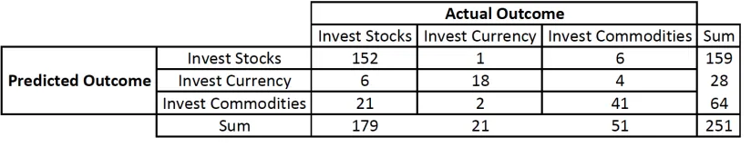
Table 3.6: Confusion Matrix for Neural Network in Bear Market

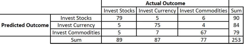
Table 3.7: Confusion Matrix for Logistic Regression in Bear Market

Neural Network, 84.8% for the logistic regression and 84% for the decision tree. Looking

at the performance in the first quarter as discussed, these results provide some basis to

in-dicate why the Logistic Regression and Decision Tree performed better. Furthermore, the

False Positives in commodities for the Neural Network was the highest at 17 compared to

12 False Positives obtained by the other two tools investigated. The specificity is calculated

to be 89.8% for the Neural Network, 94.3% for the logistic regression and 92.1% for the

decision tree, further highlighting the performance of the Logistic Regression tool. Lastly,

the performance edge in the months of November and December where the Logistic

Re-gression portfolio outperforms Decision Tree and Neural Network, could also be attributed

to the improved precision and specificity.

3.3.3

Volatile Market

A volatile market unlike the bear and bull market does not trend significantly up or down.

This type of market has a tendency to rise or fall rapidly in a short period of time. As

a result, investing and liquidating investments at the opportune time is key to maintain a

Table 3.8: Confusion Matrix for Decision Tree in Bear Market

Index, there is significant movement in both directions of up to 3.5%. Between the months

of August and November, the market dips 9.3% but is able to recover all these losses by the

start of November. Figure 3.2 presents these market conditions by plotting the S & P 500

Index and compares the performance of the data mining algorithms in 2015.

Figure 3.3: This figure presents the resulting portfolio value change over the fiscal year 2015. The change in value of the assets identified by the three classification techniques are presented with a stock market focused investment tool and the S & P 500 Index for comparison.

Considering that the Index is weighted, these fluctuations indicate strong, quick

several dips in the value of the portfolio such as March 25th or May 6th. These occurrences

upon deeper investigation were caused by the sudden nature of the share price dropping

intra-day. Next, either the classification tool or the investment strategy of limiting losses

to 5% triggers liquidation of the asset. Looking at the notional values of the portfolios, the

standalone classifier produced returns of roughly 26.8%. The neural network tool produced

a return of 23.1%, the logistic regression tool produced a return of 21% and lastly the

de-cision tree produced a return of 27.8%. A quarterly breakdown of each tool investigated is

highlighted in Table 3.9.

The results indicate that overall the Decision Tree performed the best, relying on a

sig-nificant appreciation of its assets between the months of May and August. These results

were produced with a significant distribution in stocks, most notably in Goldman Sachs.

This performance was followed closely by the stand alone stock classifier. Right after this

steady appreciation between May and August, the stock market tumbles. Again, the

Deci-sion Tree and stand alone stock classifier represent this crash by the portfolio losing value.

Much like the Bear year test scenario, the Neural Network had shifted the investments into

currencies at this point and avoid the crash. The Decision Tree follows ensuite, and invests

aggressively into currencies avoiding the impact from the slump in the stock market.

Table 3.9: Portfolio Values in Bear Market per Quarter 2008

Date Neural Network Logistic Regression Decision Tree Stock Classifier S&P 500

1/2/15 100000 100000 100000 100000 100000 3/31/15 111050.28 105332.40 110304.52 111319.61 100470.79 6/30/15 115727.25 115912.47 121373.84 117431.31 100238.56 9/30/15 119955.25 121192.84 127886.26 120088.28 93286.85 12/31/15 123121.63 121029.24 127758.91 126754.83 99307.16

Another key investment decision by all three algorithms was to invest in commodities

at the start of the fiscal year. The performance of the Neural Network and Decision Tree

at the end of the first quarter are similar at 11.1% and 10.3% respectively. The Logistic

Regression model on the other hand only presents a return of 5.3% at this time period.

copper and crude. These two assets produced a gradual return over the first three months,

unlike the investments in gold and silver also utilized by the other tools. This is reflected in

the confusion matrices in Tables 3.10-3.12. From these tables the Precision of commodities

can be calculated 70% for the Neural Network, 61.3% for the Logistic Regression and

70.6% for the Decision Tree. The specificity for the same three tools remains comparable

at 95.8% for the Neural Network, 94.4% for the Logistic Regression and 95.3% for the

Decision Tree tool.

Another point of divergence observed between the classification tools investigated is

the choice of investments after the market crash between August and November. From

Figure 3.3, it is observable that at the start of October, the stock market initiates its

recov-ery. This recovery is reflected in the stand alone stock classifier, appreciating from a value

of 120088.28 to a peak of 130735.57 as of November 20th_{. The Neural Network’s}

perfor-mance also replicates this trend, choosing to invest in stocks. The decision tree on the other

hand was unable to invest into stocks as the portfolio was invested in currencies at that

point and due to the investments being stuck in the 10% appreciation and 5% depreciation

limits, the gains were unrealized. A key point to note at this juncture is that the precision

for stocks by the decision tree was at 85.1% where as the Neural Network was marginally

lower at 84%. Hence it can be inferred that in this scenario, due to the prior investment

commitments the precision is not always a guarantee of performing the best.

Table 3.11: Confusion Matrix for Logistic Regression in Volatile Market

Table 3.12: Confusion Matrix for Decision Tree in Volatile Market

3.4

Equal Distribution in Three Assets

In this scenario, the top level classification is bypassed for the initial distribution to

vali-date if the initial distribution would impact the resulting gain on the portfolio. Utilizing

figure 3.4 to identify the results, it can be observed that despite the change in initial

distri-bution and its associated gains, ultimately the investment decisions were fairly consistent

after February and December. The Decision Tree again produced the best results, a gain

of 31.3% in this scenario compared to a gain of 27.8% previously in the dynamic

alloca-tion scenario based on the volatile market. The Neural Network produced the second best

gains, a return on 25.3%, besting the return of 23.1%. Lastly, the Logistic Regression

port-folio also improved, producing a return of 22.5%, greater than the 21% return observed

previously. These results are summarized in Table 3.13.

Table 3.13 highlights the gains made per quarter in 2015. At the end of the first

quar-ter, the Neural Network portfolio increased by $2,135.5, the Logistic Regression portfolio

increased in value by $1493.5 and the decision tree increased in value by $3533.1. Having

Figure 3.4: This figure presents the resulting portfolio value change over the fiscal year 2015 where the initial distribution of assets was evenly split between the asset classes. The change in value of the assets identified by the three classification techniques are presented with a stock market focused investment tool and the S & P 500 Index for comparison.

the currency exchange assets of USD/AUD, USD/GBP, USD/EUR had some gains in early

2015. The Decision Tree invested significantly in the USD/EUR category to boost its gains

and the Neural Network invested equally in all three currency exchange options.

Considering that the top level classifier was suspended for the initial distribution, this

scenario provides a good opportunity to evaluate the performance of the asset level

classi-fiers, classifying between buy, hold, or selling of any particular investment. Tables 3.14 to

3.16 represent the calculated Precision and Specificity of each asset class split by the

clas-sification tool employed. Specific results include the Decision Tree being the most precise

when buying any of the three asset types, this is most prominent in the currencies asset

type with a precision of 80.4%. The Logistic Regression tool performs the worst across

all three asset types, dropping its precision to 66.1% when buying commodities. Lastly,

Table 3.13: Portfolio Values in Volatile Market per Quarter 2015 with Split Initial Distri-bution

Date Neural Network Logistic Regression Decision Tree Stock Classifier S&P 500

1/2/15 100000 100000 100000 100000 100000 3/31/15 112567.678 106866.7847 113354.9071 111319.6133 100470.7969 6/30/15 115560.6036 117857.4849 124730.3389 117431.3157 100238.5655 9/30/15 122035.8742 121192.8419 129248.5931 120088.284 93286.85622 12/31/15 125257.1824 122522.7466 131291.986 126754.8379 99307.1611

averaged across the three asset classes.

Table 3.14: Performance Evaluation for Stock Level Classifier

3.4.1

Review

The hypothesis stated that implementing a multi-asset portfolio with a two stage

classifi-cation setup would yield in greater returns than a regular stock based classificlassifi-cation tool.

Reviewing the results, in the bull market, the stand alone stock classifier outperformed the

implementations investigated in this study. In a bull market, results indicate that majority

of the time investing in stocks is the best option. The bear and volatile markets allow for

further analysis of the implementation. In the bear market, all three tools comprehensively

outperformed the stock based classifier, achieved by altering investments from stocks to

currencies at specific points in the fiscal year. Lastly, the volatile market produced another

validation, with the decision tree performing the best. In this scenario the stock classifier

Table 3.15: Performance Evaluation for Commodity Level Classifier

Table 3.16: Performance Evaluation for Currency Level Classifier

The use of precision and specificity derived from confusion matrices helped identify

useful trends such as the logistic regression performing poorly in the volatile market

sce-nario. This particular classification technique had the lowest precision and appropriately

reflected on the net gain in that portfolio. Having stated this fact, it was also observed

that despite the Decision Tree having the best precision in the same scenario, due to prior

investments it was unable to liquidate and re-invest itself into a better performing asset.

Ultimately investigating these observances, exploring a wider set of products and flattening

the two level classifier into a single level classifier will further strengthen the hypothesis.

Chapter 4

Conclusions

4.1

Current Status

This report demonstrates that a multi-asset based portfolio backed by decisions made using

data mining techniques provides improved performance in many market scenarios when

compared to a stand alone stock classifier. The application framework outlined in the

hy-pothesis and subsequently tested upon functions as outlined in the report. There are some

incomplete operational aspects, improving these aspects could lead towards creating a

bet-ter application and experience for the end user. A list of these aspects include the following

items:

• Tighter integration between the R based tools and the Java application - Currently the .CSV training and test files are manually loaded into the R application and

subse-quently loaded in to the Java Application for portfolio maintenance. Localizing the

classification tools into the Java application will allow for a stand alone application.

• Investigate/Subscribe to data sources - A significant subset of the data used to train and validate the analytical tools investigated in this study is paid and free data is often

more periodical. Exploring paid sources of reliable data will streamline training and

testing dataset creation.

• Improve output of asset decisions to visual cues - Currently the final Java Application

portfolio. For and end user using this application to invest, the output should be

altered to state instructions on what actions to take.

These operational updates highlight some improvements that will aid the ultimate

us-ability of the application created in this study. The next section outlines some function

aspects to investigate further to strengthen the hypothesis validation.

4.2

Future Work

The testing and hypothesis validation performed in this study have demonstrated that a

multi-asset portfolio in many market scenarios builds on a stand alone stock classifier and

can help mitigate economic and market risks for new investors, however there are some

further avenues to research to improve and fine tune the resulting solution.

To limit the scope of this study the products available to invest were the: 30 Stocks in

the Dow Jones Industrial Average, top 10 most traded currency pairs, and the top 10 most

traded commodities. Widening the range of these products will help reduce any inherent

bias introduced by limiting the choice. Considering that the 30 Stocks in the Dow Jones

Industrial Average are themselves chosen on a unique set of economic criteria, a wider set

would help increase the diversity in both the training set and risk mitigation.

Another aspect that can be further investigated is the ability to short sell or use the

alternate currency exchange pair, allowing the investor to bet against the market. Short

selling involves selling a borrowed set of stocks with the motivation that the price will

drop. Once the price has dropped, it can be bought and returned to the loaner, allowing the

investor to utilize the differential. Reverse currency exchange follows the same principle,

utilizing borrowed foreign funds to bet against the US Dollar.

This study also utilized the 10% appreciation and 5% depreciation limits as a trading

strategy coupled with the 30 day forced liquidation. To validate the hypothesis more

rigor-ously, all three factors must be manipulated. In some test scenarios reflected in this study,

the investment choices, if the portfolio is already distributed and unable to re-invest, greater

returns could be missed.

The top level training set utilized to distinguish between the three asset classes in this

study utilized a training set based on the S & P 500 Index and custom currency and

com-modities index. These two indexes were weighted by the volume, creating a buffered index.

Hence in some scenarios it is observable that although one sub asset like crude oil may be

performing well, if other commodities are not performing well, this investment choice may

be excluded. Hence future studies should investigate flattening the two level classification

tool, and identifying best investment choices as a comparison to the two stage method

uti-lized in this study. Additionally this study utiuti-lized three market scenarios, often providing

distinct choices between investment categories. More market scenarios must be validated

against to investigate the effectiveness of the solution.

4.3

Lessons Learned

The testing and analysis in this study has presented that unless in a bull market scenario,

utilizing a multi-asset portfolio with a data mining tool can prove beneficial to a novice

investor. In a bear market, this study outlined how the performance of the multi-asset

port-folio is drastically better than investing using a standalone stock classifier or investing in an

index tracked product. In a volatile market, this study showed that a multi-asset portfolio

is competitive with a standalone stock classifier and in many scenarios even out perform

it. Looking at the underlying data mining techniques used and test results, the Logistic

Regression preformed best when long term trends were available. The Decision Tree and

Neural Network performed better in volatile market conditions, owing to better fitting to

that training data set. Lastly, a key point that although the tool utilized may be the most

precise in that scenario, ultimately the trading strategy and existing investment decisions

can also impact the gains made. Overall, based on the results and issues identified, this

study provides a good basis to build further research upon. Ultimately, the end goal would

Bibliography

[1] Kan Deng. OMEGA: On-line memory-based general purpose system classifier. PhD thesis, Georgia Institute of Technology, 1998.

[2] Ehsan Hajizadeh, Hamed Davari Ardakani, and Jamal Shahrabi. Application of data mining techniques in stock markets: A survey. Journal of Economics and Interna-tional Finance, 2(7):109, 2010.

[3] Carol Anne Hargreaves, Prateek Dixit, and Ankit Solanki. Stock portfolio selection using data mining approach. IOSR Journal of Engineering (IOSRJEN), 3(11):42–48, 2013.

[4] Imran Kurt, Mevlut Ture, and A Turhan Kurum. Comparing performances of logis-tic regression, classification and regression tree, and neural networks for predicting coronary artery disease. Expert Systems with Applications, 34(1):366–374, 2008.

[5] S. S. Patel. Should you trade stocks on your iphone? - marketwatch, 2014. [Online; accessed 6-January-2015].

[6] Apostolos-Paul Refenes. Neural networks in the capital markets. John Wiley & Sons, Inc., 1994.

[7] Ra´ul Rojas.Neural networks, a systematic introduction. Springer Science & Business Media, 2013.

[8] David E Rumelhart, Geoffrey E Hinton, and Ronald J Williams. Learning represen-tations by back-propagating errors. Cognitive modeling, 5(3):1, 1988.

[9] Linda Shapiro. Information Gain. University of Washington, 1999.

[10] Efraim Turban, Ramesh Sharda, Jay E Aronson, and David King. Business intelli-gence: A managerial approach. Prentice Hall, 2008.