Hierarchical Gaussian Process Priors
.
White Rose Research Online URL for this paper:
http://eprints.whiterose.ac.uk/135555/
Version: Accepted Version
Article:
Kuzin, D., Isupova, O. and Mihaylova, L. orcid.org/0000-0001-5856-2223 (2018)
Spatio-Temporal Structured Sparse Regression With Hierarchical Gaussian Process
Priors. IEEE Transactions on Signal Processing, 66 (17). pp. 4598-4611. ISSN 1053-587X
https://doi.org/10.1109/TSP.2018.2858207
[email protected] https://eprints.whiterose.ac.uk/
Reuse
Items deposited in White Rose Research Online are protected by copyright, with all rights reserved unless indicated otherwise. They may be downloaded and/or printed for private study, or other acts as permitted by national copyright laws. The publisher or other rights holders may allow further reproduction and re-use of the full text version. This is indicated by the licence information on the White Rose Research Online record for the item.
Takedown
If you consider content in White Rose Research Online to be in breach of UK law, please notify us by
Spatio-Temporal Structured Sparse Regression with
Hierarchical Gaussian Process Priors
Danil Kuzin, Olga Isupova, and Lyudmila Mihaylova,
Senior Member, IEEE
Abstract—This paper introduces a new sparse spatio-temporal structured Gaussian process regression framework for online and offline Bayesian inference. This is the first framework that gives a time-evolving representation of the interdependencies between the components of the sparse signal of interest. A hierarchical Gaussian process describes such structure and the interdependencies are represented via the covariance matrices of the prior distributions. The inference is based on the expecta-tion propagaexpecta-tion method and the theoretical derivaexpecta-tion of the posterior distribution is provided in the paper. The inference framework is thoroughly evaluated over synthetic, real video and electroencephalography (EEG) data where the spatio-temporal evolving patterns need to be reconstructed with high accuracy. It is shown that it achieves 15% improvement of the F-measure compared with the alternating direction method of multipliers, spatio-temporal sparse Bayesian learning method and one-level Gaussian process model. Additionally, the required memory for the proposed algorithm is less than in the one-level Gaussian process model. This structured sparse regression framework is of broad applicability to source localisation and object detection problems with sparse signals.
I. INTRODUCTION
S
PARSE regression problems arise often in various ap-plications, e.g., compressive sensing [1], EEG source localisation [2] and direction of arrival estimation [3]. In all these applications, a dictionary of basis functions can be constructed that allows sparse representations of the signals of interest, i.e. many of the coefficients of the basis functions are close to zero. This allows to perform sensing tasks with lower amount of observations than the signal dimensionality. However, the signal recovery problem becomes more computationally expensive when sparsity assumptions are incorporated.The sparse signal representation can be expressed as a regression problem of finding a signal x given the vector
y of observations and the design matrix Athat satisfies the equation
y=Ax+ε, (1)
where ε is the Gaussian noise vector, ε∼ N(ε;0, σ2I), σ2
is the variance and I is the identity matrix. Therefore, the observations also have a Gaussian distribution
y∼ N(y;Ax, σ2I). (2)
When the number of observations is less than the number of coefficients the problem is ill-posed in the sense that it has
D.Kuzin, L.Mihaylova are with the Department of Automatic Control and Systems Engineering, the University of Sheffield, Sheffield, UK e-mail: [email protected], [email protected]. O.Isupova is with the Department of Engineering Science, the University of Oxford, Oxford, UK e-mail: [email protected]
an infinite number of possible solutions and additional regu-larisation is required. This is usually achieved by imposinglp
penalty functions with0≤p <2[4], [5], [6].
In the compressive sensing literature, it has been shown that if a matrix A satisfies the restricted isometry property (RIP) [7] then a solution of a convexl1-minimisation problem
is equivalent to a solution of a sparsel0-minimisation problem.
However, the problem of identification whether a given matrix satisfies the RIP is NP-hard [8]. In contrast, Bayesian models do not impose any restrictions on the matrixA and regularise the problem (1) with sparsity-inducing priors [9].
Bayesian models for sparse regression can be classified into models with aweak sparsity prior and astrong sparsity
prior [10]. The weak sparsity prior leads to a unimodal posterior distribution of the signal with a sharp peak at zero, thus each coefficient has a high posterior probability of being close to zero. The strong sparsity prior is a mixture of latent binary variables that explicitly capture whether coefficients are zero or non-zero. In this paper we consider one type of strong sparsity priors — spike and slab models.
In spike and slab models, sparsity is achieved by selecting each component ofxfrom a mixture of a spike distribution, that is the delta function, and a slab distribution, that is some flat distribution, usually a Gaussian with a large variance [11]. Following the Bayesian approach, latent variables that are indicators of spikes are added to the model [12] and a relevant distribution is placed over them [13]. Therefore, each signal component has an independent latent variable, which controls whether this component would be a spike or a slab.
In many applications, the independence assumption is not valid [14] as non-zero elements tend to appear in groups, and an unknown structure often exists in the field of the latent variables. For example, wavelet coefficients of images are usually organised in trees [15], chromosomes have a spatial structure along a genome [16], video from single-pixel cameras has a temporal structure [17]. In these cases it is useful to introduce additional hierarchical or group penalties that promote such structures in recovered signals.
A. Contributions
This paper proposes the spike and slab model with a hierarchical Gaussian process prior on the latent variables. Such hierarchical prior allows to model spatial structural dependencies for signal components that can evolve in time.
The model has a flexible structure which is governed only by the covariance functions of the Gaussian processes. This allows to model different types of structures and does not require any
specific knowledge about the structure such as determination of particular groups of coefficients with similar behaviour. If, however, there is information about the structure, it can be easily incorporated into the covariance functions. The model is flexible as spatial and temporal dependencies are decoupled by different levels of the hierarchical Gaussian process prior. Therefore, the spatial and temporal structures are modelled independently allowing to encode different assumptions for each type of structure. It allows to reduce complexity and process streaming data.
Overall, the main contributions of this work consist in: 1) the proposed novel spike and slab model with the
hierarchical Gaussian process prior for signal recovery with spatio-temporal structural dependencies;
2) the developed Bayesian inference algorithm based on expectation propagation;
3) the novel online inference algorithm for streaming data based on Bayesian filtering;
4) a thorough validation and evaluation of the proposed method over synthetic and real data including the electrical activity data for the EEG source localisation problem and video data for the compressive background subtraction problem.
The paper is organised as follows. Section II reviews the related work. Section III provides an overview of existing spike and slab models. The proposed model and the inference algorithm are presented in Section IV. Section V demonstrates the online version of the algorithm. Section VI presents the complexity evaluation and numerical experiments. Section VII concludes the paper. Appendices provide theoretical derivations of the inference algorithm.
II. RELATED WORK
Different spatial structure assumptions for sparse models have been extensively studied in the literature. The group lasso [18], [19] extends the classical lasso method for group sparsity such that coefficients form groups and all coefficients in a group are either non-zero or zero together, but groups are required to be defined in advance. In contrast to group lasso, structural dependencies in our model are defined by the parameters of covariance functions of the Gaussian processes (GPs) and the actual groups are inferred from the data.
Group constraints for weak sparse models include smooth relevance vector machines [20], spatio-temporal coupling of the parameters for the scale mixture of Gaussians repre-sentation [21], [22], row and element sparsity [23], block sparsity [24].
For spike and slab priors a spatio-temporal structure is modelled with a one-level Gaussian processes prior [25], where the prior is imposed on all locations of non-zero components together. The covariance matrix is represented as the Kronecker product of the temporal and spatial matrices.
In contrast to the one-level GP our model introduces an additional level of a GP prior for temporal dependencies. Therefore, the temporal and spatial structures are decoupled. The proposed model is thus more flexible. Broadly speaking, the top-level GP can encode the slow change of groups of
spikes positions in time while the low-level GP allows to model the local changes of each group. The one-level GP prior model also requires significantly more memory to store the covariance function for modelling both spatial and temporal structural dependencies as it is built as a Kronecker product of spatial and temporal covariance matrices. The resulting size of the covariance matrix scales quadratically with spatio-temporal dimensionality, which makes it infeasible even for average size problems, whereas for our model the total size of two covariance matrices scales linearly.
More importantly, in the proposed model structural depen-dencies are considered at every timestamp whereas in [25] the GP prior is imposed on the whole batch of data. This consideration of every timestamp allows us to develop an incremental inference algorithm — all latent variables are inferred for the new time moment in the similar manner as for the offline inference. Meanwhile, it is unclear how to apply the one-level GP model to the incremental data without re-processing the previous data.
GPs are widely used to model complex structures and dynamics in data not only in sparse problems. In [26] GP is used as a prior for nonlinear state transition and observation functions for state-space Bayesian filtering. Hierarchical GP models are proposed to model structures in [27].
III. SPARSE MODELS FOR STRUCTURED DATA
This section presents a roadmap of models that are used in the formulation of the proposed spatio-temporal structured sparse model. It starts from the basic spike and slab model and continues with its extension for structured data.
The generative model for the spatio-temporal regression problem can be formulated in the following way:
• The data is collected for the sequence of theT discrete timestamps. Indexes are denoted byt∈[1, . . . , T].
• At each timestampt the unknown signal of sizeN is de-noted byxt= [x1t, . . . , xN t]⊤. Signals at all timestamps
are concatenated into a matrixX= [x1, . . . ,xT].
• The observations of size K are denoted by yt = [y1t, . . . , yKt]⊤. They are obtained with the design matrix
A∈RK×N. Observations at all timestamps are concate-nated into matrixY= [y1, . . . ,yT].
• An independent Gaussian noise with the varianceσ2 is
added to the observations.
The probabilistic model can be then expressed as
p(yt|xt) =N(yt;Axt, σ2I) ∀t. (3)
It is assumed that the dimensionality K of observations yt
is less than the dimensionality N of signals xt, therefore
the problem of recovery of signalxt from observationsyt is
underdetermined and it can have an infinite number of solutions. Sparsity-inducing priors allow to specify additional constraints that lead to a unique optimal solution.
A. Factor graphs
models. They are also important for the approximate inference method described in Section IV.
The joint probability density function p(·) of latent vari-ablesζi can be factorised as a product of factorsψC that are
functions of a corresponding set of latent variablesζC
p(ζ1, ..., ζm) =
1
Z
Y
C
ψC(ζC), (4)
where Z is a normalisation constant. This factorisation can be represented as a bipartite graph with variable vertices corresponding to ζi, factor vertices corresponding toψC and
edges connecting corresponding vertices.
The distribution of latent variables xt in (3) can be
repre-sented as a factor
gt(xt) =N(yt;Axt, σ2I). (5)
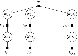
The factor graphs are used in this paper to visualise different spike and slab models. In Fig. 1 – 3 circles represent variable vertices and small squares represent factor vertices.
B. Spike and slab model
Sparsity can be induced with the spike and slab model [29], where additional latent variables Ω = {ωit}t=1:T , i=1:N
indicate if signal componentsxitare zeros. This is represented
as a mixture of a spike and a slab
p(xit|ωit) =ωitδ0(xit) + (1−ωit)N(xit; 0, σ2x), (6)
where spikeδ0(·) is the delta function centered at zero, and
slab is the Gaussian distribution with the variance σ2
x. The
conditional distributions p(xit|ωit) are further denoted by
factorsfit(ωit, xit).
In this model {ωit}i=1:N are considered conditionally
independent given xt. The prior is imposed on the indicators
p(ωit) =Ber(ωit;z), (7)
where Ber(·;z)denotes a Bernoulli distribution with the success probability parameter z. The prior distributions p(ωit) are
further denoted by hind
it (ωit). The problem (5) – (7) can be
solved independently for each t.
The model can be represented as a factor graph (Fig. 1) with a product of factors (5) – (7) for allt andi.
The posteriorp(X,Ω)of latent variablesXandΩis
p=
T
Y
t=1
"
gt(xt) N
Y
i=1
fit(ωit, xit)hindit(ωit)
#
. (8)
C. Spike and slab model with a spatial structure
A spatial structure can be implemented by adding interdepen-dencies for the locations of spikes in xit [25], [30], [31]. This
is achieved by modelling the probabilities of spikes with the ad-ditional latent variables Γ= [γ1, . . . ,γT] ={γit}t=1:T , i=1:N
that are samples from a Gaussian process. A Gaussian process is a way to specify prior on functions, it can be defined as an infinite expansion of multivariate Gaussian distribution. In GP all finite subsets of variables have a joint Gaussian distribution. The properties of the structure are defined through
x1t x2t . . . xN t
ω1t ω2t ωN t
gt
f1t f2t fN t
[image:4.612.358.524.58.178.2]h1t h2t hN t
Fig. 1. Spike and slab model for one time moment (different time moments are independent). All signal components are conditionally independent given data, therefore structural assumptions cannot be modelled.
the covariance function of GP, which in this paper is assumed to be squared exponential:
p(γt) =N(γt;µt,Σ0),Σ0(i, j) =αΣexp
−(i−j) 2
2ℓ2 Σ
,
(9) where µt is the mean vector and Σ0 is the covariance matrix
with the hyperparametersαΣ andℓ2Σ.
The conditional independence assumption forωitfrom (7)
is replaced by
p(ωit|γit) =Ber(ωit; Φ(γit)), (10)
p(γt) =N(γt;µt,Σ0), (11)
where Φ(·) is the standard Gaussian cumulative distribution function (cdf). Scaling is required to normalise probabilities to the[0,1]interval and it is convenient to useΦ(·)for this purpose in the derivations with GPs [32]. The conditional distributions p(ωit|γit) are denoted by factors hit(ωit, γit).
The prior distributionsp(γt)are denoted by rind
t (γt).
In this model{γt}t=1:T are independent and therefore the
problem can be solved separately for each timestamp. Using the introduced factors (5), (6) and (10) – (11), factor graph can be built as in Figure 2. The posteriorp(X,Ω,Γ) of the latent variables is given by
p=
T
Y
t=1
"
gt(xt) N
Y
i=1
[fit(ωit, xit)hit(ωit, γit)]rt(γt)
#
. (12)
IV. THE PROPOSED SPATIO-TEMPORAL STRUCTURED SPIKE AND SLAB MODEL
In this paper a spatio-temporal latent structure of the positions of non-zero signal components is considered for the underdetermined recovery problem (3). The following assumptions are introduced:
1) xt is sparse, i.e. it contains a lot of zeros for each
timestampt;
2) non-zero elements in xtare clustered in groups for each
timestampt;
3) these groups can move and evolve in time.
x1t x2t . . . xN t
ω1t ω2t ωN t
γ1t γ2t γN t
gt
f1t f2t fN t
h1t h2t hN t
[image:5.612.95.262.57.216.2]rt
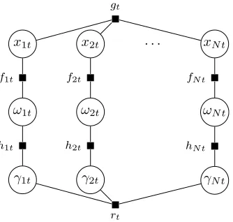
Fig. 2. Spike and slab model with a spatial structure for one time moment. The locations of spikes have a GP distribution, therefore encouraging a structure in space, but they are independent in time.
can be implemented in the model using the spike and slab prior (6).
Similarly to Section III-C, the second model assumption can be implemented by adding spatial dependencies for the positions of spikes inxit. This is achieved by modelling the
probabilities of spikes Ω with the scaled GP onΓ (10), (11). GPs specify a prior over an unknown structure. This is particularly useful as it allows to avoid a specification of any structural patterns — the only parameter for structural modelling is the GP covariance function.
The third condition is addressed with the dynamic hierarchi-cal GP prior. The mean M= [µ1,. . . ,µT]for the spatial GP
evolves over time according to the top-level temporal GP
µt∼ N(µt;µt−1,W),W(i, j) =αWexp
−(i−j) 2
2ℓ2
W
,
(13) whereW is the squared exponential covariance matrix of the temporal GP with the hyperparameters αW andℓ2W.
This allows to implicitly specify the prior over the evolution function of the structure. The rate of the evolution is controlled with the top-level GP covariance function.
According to these assumptions, the model can be expressed as a factor graph (Figure 3) where the factor rt(γt,µt)
denotes N(γt;µt,Σ0) and the factor ut(µt,µt−1) denotes N(µt;µt−1,W).
The full posterior distribution p(X,Ω,Γ,M)is then
p=
T
Y
t=1
"
gt(xt) N
Y
i=1
[fit(xit, ωit)hit(ωit, γit)]rt(γt,µt)
#
×
T
Y
t=2
ut(µt,µt−1). (14)
The exact posterior for the proposed hierarchical spike and slab model is intractable, therefore approximate inference methods should be used. In this paper expectation propaga-tion (EP) [33] is employed. EP is shown to be the most effective Bayesian inference method for sparse modelling [34].
In this section the description of the EP method and the key components of the inference for the proposed model are
presented. The details of the inference algorithm can be found in the appendices.
A. Expectation propagation
EP is a deterministic inference method that approximates the posterior distribution using the factor decomposition (4), where each factor is approximated with distributionsψ˜C(·) from the
exponential family:
˜
p(ζ1, ..., ζm) =
1 ˜
Z
Y
C
˜
ψC(ζC), (15)
where p˜ is an approximating distribution and Z˜ is a nor-malisation constant. Approximating factorised distribution is determined by minimisation of the Kullback-Leibler (KL) divergence with the true distribution. The KL-divergence is a common measure of similarity between distributions.
Direct approximation is intractable due to intractability of the true posterior. Minimisation of the KL divergence between individual factorsψC and ψ˜C may not provide good
approximation for the resulted product. In EP, approximation of each factor is performed in the context of other factors to improve a result for the final product. Iteratively one of the factors is chosen for refinement. The chosen factor
˜
ψC is refined to minimise the KL-divergence between the
productq ∝ψ˜CQC′=6 Cψ˜C′ and ψCQ
C′6=Cψ˜C′, where the
approximating factor is replaced with a factor from the true posterior.
Factor refinement consists of five steps which are summarised below (with details given in Appendices B-E).
1) Compute a cavity distribution q\C ∝ q
˜
ψC
: the joint
distribution without the factorψ˜C
2) Compute a tilted distributionψCq\C: the product of the
cavity distribution and the true factor
3) Refine the approximationq:q∗=argmin KL ψ
Cq\C||q
by minimising the KL-divergence between the tilted distribution ψCq\C and the approximating distributionq.
This is equivalent to matching the moments of the distributions [33].
4) Compute an updated factorψ˜new
C ∝
q∗
q\C using the refined
approximation and cavity distribution.
5) Update the current joint posterior qnew ∝ ˜
ψnew
C
Q
C′6=Cψ˜C′ with the newly updated factor
˜
ψnew
C .
B. Approximating factors
Here the key components of the EP inference algorithm for the proposed model are provided. The true posteriorp(14) is approximated with the distribution q
q=Y
t
qgtqftqhtqrtqut, (16)
where each factor qa, a ∈ {gt, ft, ht, rt, ut}, is from the
x1t x2t · · · xN t
ω1t ω2t ωN t
γ1t γ2t γN t
· · · ·
µt−1 · · ·
µ1 µt µt+1 · · · µT
· · · ·
gt
f1t f2t fN t
h1t h2t hN t
rt
[image:6.612.150.466.57.218.2]u2 ut−1 ut ut+1 ut+2 uT
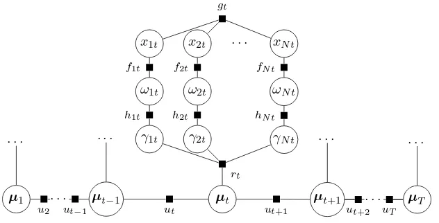
Fig. 3. Proposed spike and slab model with a spatio-temporal structure. The locations of spikes have a GP distribution in space with parameters that are controlled by a top-level GP and they evolve in time, therefore promoting temporal dependence.
Below the factors qa of the approximating posterior qare
introduced. Gaussian and Bernoulli distributions are used in the factors, which parameters are updated during the iterations of the EP algorithm.
The factors gt=N(yt;Axt, σ2I)from (5) can be viewed
as the distributions of xt with fixed observed variables yt:
qgt = N(xt;mgt,Vgt), where mgt = (A
⊤A)−1A⊤y
t,
Vgt=σ2(A⊤A)−1.
The factors ft = QNi=1fit and ht = QNi=1hit from (6)
and (10) are approximated with the products of Gaussian and Bernoulli distributions
qft =N(xt;mft,Vft)
N
Y
i=1
Ber(ωit; Φ(zfit)), (17)
qht =N(γt;νht,Sh)
N
Y
i=1
Ber(ωit; Φ(zhit)), (18)
where the components ofxtandγtare independent. Therefore,
the covariance matricesVft andShare diagonal
1
. Distribution parameters mft, Vft, zfit, νht, Sh, and zhit are updated
during EP iterations according to Appendices B and C. The approximation for the factors rt=N(γt;µt,Σ0)and ut=N(µt;µt−1,W)from (9) and (13) is intended to separate
the latent variables and it is represented as products of Gaussian distributions
qrt =N(γt;νrt,Sr)N(µt;ert,Dr), (19) qut =N(µt−1;eut←,Du←)N(µt;eut→,Du→). (20)
Distribution parametersert,Dr,νrt,Sr,eut←,Du←,eut→,
and Du→ are updated during EP iterations according to
Appendices D and E.
The posterior approximation qgiven by (16) thus contains the products of Gaussian and Bernoulli distributions that are equal to unnormalised Gaussian and Bernoulli distributions, respectively (Appendix A). This can be conveniently expressed
1Note thatS
hdoes not depend on time. In this paper, single covariance
matrices are used for all time moments for both GP variablesγandµin the
approximating factors. However, the method can be applied with individual covariance matrices for each time moment as well.
in terms of the natural parameters andqcan be represented in terms of distributions of the latent variables.
For xt in q this product property leads to the Gaussian distributionN(xt;mt,Vt)with natural parameters
Vt−1=V−g1
t +V
−1
ft ,V
−1
t mt=Vg−t1mgt+V
−1
ft mft. (21)
Similarly, γt in q is distributed as N(γt;νt,S), where
natural parameters are
S−1=S−h1+S−r1,S−1νt=S−h1νht+S
−1
r νrt. (22)
The top GP latent variablesµthave the Gaussian distribu-tionsN(µt;et,D)with natural parameters
D−1=D−r1+Du−→11t>1+D−u←11t<T, (23a)
D−1et=D−r1ert+D
−1
u→eut→1t>1+
D−u←1eut+1←1t<T, (23b)
where1is the indicator function.
The distributions forωtareQNi=1Ber(ωit; Φ(zit))with the
parameters
zit= Φ−1
(1−Φ(zfit))(1−Φ(zhit))
Φ(zfit)Φ(zhit)
+ 1 −1!
. (24)
The full approximating posteriorq is then
q=
T
Y
t=1
N(xt;mt,Vt)
T
Y
t=1
N
Y
i=1
Ber(ωit; Φ(zit))
×
T
Y
t=1
N(γt;νt,S) T
Y
t=1
N(µt;et,D). (25)
In the EP inference algorithm, each of the introduced approximating factorsqft,qht,qrt,qut is iteratively updated
according to the factor refinement procedure as in Section IV-A. Note that the factorsqgt are not updated, as the corresponding
factorsgtfrom the true posterior distribution are already from
C. Implementation details
There are no theoretical guarantees of EP convergence. However, it can be achieved usingdamping[35]: during step 4 of the factor refinement procedure in Section IV-A the factor is updated asqdampa = (qnewa )η(qolda )1−η, whereqaold is the value
of the factor from the previous iteration, qnew
a is the updated
value of the factor, η ∈ (0,1] is the damping coefficient. It is exponentially decreased as η =ηoldξ
after each iteration, where ξ ∈(0,1] is the parameter that governs the speed of exponential decrease and ηold
is the value of the damping coefficient from the previous iteration.
It is also known that during the EP updates negative variances can appear [34]. In this case negative variances are replaced with a large value representing+∞.
V. ONLINEINFERENCE WITHBAYESIANFILTERING In this section the problem (3) is considered for streaming data, i.e. when new data becomes available at every timestamp. The conventional batch inference can be infeasible for large or streaming data. The developed online Bayesian filtering algorithm for the model presented in Section IV allows to iteratively update the approximation ofxbased on new samples of data.
Bayesian filtering consist of two steps that are iterated for each new sample of data:
• prediction, where an estimate of a hidden system state at the next time step is predicted based on the observations available at the current time moment;
• update, where this estimate is updated once an observation at the next time moment is obtained.
In the proposed model the hidden state is represented by the latent variablesxt,ωt,γtandµtthat should be inferred based
on observations yt.
A. Prediction
At the prediction step for the timestamp t+ 1the current estimate of the posterior distribution of the latent variables
p(xt,ωt,γt,µt|y1:t) is available. It is based on all
observa-tions y1:t = [y1,. . . ,yt] up to the timestamp t. The initial
estimate of this posterior can be obtained by the offline inference algorithm applied to the initialTinit timestamps.
Marginalisation of the latent variables for the current timestamptallows to obtain predictions for the latent variables for the next timestamp t+ 1
p(xt+1,ωt+1,γt+1,µt+1|y1:t) =
= Z
p(xt+1,ωt+1,γt+1,µt+1|xt,ωt,γt,µt)
×p(xt,ωt,γt,µt|y1:t)dxtdωtdγtdµt (26)
The first term in the integral (26) is factorised according to the generative model (5),(6),(10), and (13)
p(xt+1,ωt+1,γt+1,µt+1|xt,ωt,γt,µt)
=p(xt+1|ωt+1)p(ωt+1|γt+1)p(γt+1|µt+1)p(µt+1|µt)
(27)
Therefore, the terms related to variables xt+1, ωt+1 and γt+1 are independent from the integral variables in (26) and
the integral can be rewritten as Z
p(xt+1,ωt+1,γt+1,µt+1|xt,ωt,γt,µt)
×p(xt,ωt,γt,µt|y1:t)dxtdωtdγtdµt
=p(xt+1|ωt+1)p(ωt+1|γt+1)p(γt+1|µt+1)
×
Z
p(µt+1|µt)p(µt|y1:t)dµt (28)
The initial estimate of the posteriorp(µTinit|y1:Tinit)obtained from the offline EP algorithm is a Gaussian distribution:
p(µTinit|y1:Tinit) =N(µTinit;e1:Tinit,D1:Tinit), (29)
where e1:Tinit and D1:Tinit are the mean and the covariance matrix of the estimate of the posterior forµTinit obtained based on observations y1:Tinit.
According to the generative model (13) the first term of the integral in (28) is also Gaussian, therefore the integral is also a Gaussian distribution onµt+1 for t=Tinit:
Z
p(µt+1|µt)p(µt|y1:t)dµt
=N(µt+1;e1:t,Dpredict1:t )
def
= ˆp(µt+1), (30)
where Dpredict1:t =W+D1:tis the covariance of the predicted
distribution.
Substitution of (28) and (30) back into (26) provides the predicted distribution:
p(xt+1,ωt+1,γt+1,µt+1|y1:t)
=p(xt+1|ωt+1)p(ωt+1|γt+1)p(γt+1|µt+1)ˆp(µt+1) (31)
B. Update
At the update step the predicted distribution (31) of the latent variables for the next timestamp is corrected with the new datayt+1
p(xt+1,ωt+1,γt+1,µt+1|y1:t+1)
=1
Zp(yt+1|xt+1,ωt+1,γt+1,µt+1) ×p(xt+1,ωt+1,γt+1,µt+1|y1:t)
=1
Zp(yt+1|xt+1)p(xt+1|ωt+1)p(ωt+1|γt+1) ×p(γt+1|µt+1)ˆp(µt+1), (32)
whereZ is the normalisation constant.
Since components of the vectors xt+1 and ωt+1 are
conditionally independent, the terms p(xt+1|ωt+1) and p(ωt+1|γt+1)are further factorised:
p(xt+1,ωt+1,γt+1,µt+1|y1:t+1)
=1
Zp(yt+1|xt+1)
"N Y
i=1
p(xit+1|ωit+1)p(ωit+1|γit+1)
#
×p(γt+1|µt+1)ˆp(µt+1), (33)
related toµt. The approximation of this posterior is proposed in Section IV. The algorithm is only required to be adjusted for the new factorpˆ(µt+1).
The factorpˆ(µt+1)is a Gaussian distribution, i.e. it is from
the exponential family already and it only depends on a single latent variable, therefore this factor should not be updated in the EP iterations. The information from this factor will be passed through the general approximating distribution q to the other factors.
In the EP algorithm used for inference of the updated distribution (33) the distribution for µt is approximated with the Gaussian distribution for anyt. Therefore, the identity (30) is true for anyt and the whole procedure can be applied for all timestamps.
C. Minibatch filtering
The developed Bayesian filtering procedure can be easily extended to the case of inferring minibatches for timestamps [t+ 1 :t+M], where M is the size of a minibatch:
p(xt+1:t+M,ωt+1:t+M,γt+1:t+M,µt+1:t+M|y1:t+M) (34)
rather than for the next timestamp t+ 1only as in (33). Indeed, due to conditional independence marginalisation (26) also comes down to integral (30) similar to (28). And the update step can also be performed by the EP algorithm with the only difference that it should be applied forM timestamps rather than one.
VI. EXPERIMENTS
This section presents validation and evaluation results for the proposed algorithms. The performance of these two-level GP algorithms is compared with:
• the spatio-temporal spike and slab model with a one-level GP prior and its modification with common precision approximation [25];
• a popular alternating direction method of
multipli-ers (ADMM) method [36], which is a convex optimisation method used here for the lasso problem [4];
• a spatio-temporal sparse Bayesian learning (STSBL)
algorithm [37].
For quantitative comparison, the following measures are used:
• NMSE(normalised mean square error) = kX−Xbk
2
F
kXk2
F
,
whereXis the true signal,Xb is the estimate, computed as the mean of the approximated posterior distribution,
k · kF is the Frobenius norm of a matrix;
• F-measure [13] = 2 precision·recall
precision+recall between non-zero elements of the true signalXand non-zero elements of the estimate Xb.
The NMSE shows the normalised error of signal reconstruction, with 0 corresponding to an ideal match. The F-measure shows how well slab locations are restored. An F-measure equal to 1 means that the true and estimated signals coincide, whilst 0 corresponds to lack of similarity between them. Arguably, for
10 20 30 40 50 20
40 60 80 100
time
signal
component
−200
−100 0 100 200
(a) Data
10 20 30 40 50 20
40 60 80 100
time
signal
component
−200
−100 0 100 200
[image:8.612.328.548.66.146.2](b) Data
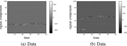
Fig. 4. Examples of the true signalXfor the synthetic data. In each example two groups of slabs generated att= 1evolve in time untilt= 50.
the sparse regression problem, the NMSE is less meaningful than the F-measure [38].
Both two-level and one-level GP algorithms are iterated until convergence, which is measured by difference in the estimate of the signalXb at the current and previous iterations.
A. Synthetic data
In this experiment, the algorithm performance is studied on synthetic data with known true values of signal X and slab locationsΩ. The synthetic data represents the signals that have slowly evolving in time groups of non-zero elements. To create a spatio-temporal structure of slabs at the first timestamp
t= 1two groups of slab locations are generated with Poisson-distributed sizes for the signalxtof dimensionalityN = 100.
Then, from t = 2 to t = T = 50, these groups randomly evolve: each border of each group can go up, down, or stay at the same location with such probabilities that in average the sparsity level remains95%. In such way, locations of the slab groups are generated. The values of non-zero elements of the signal are then drawn from the distribution N(0,104). This
procedure is repeated 10 times to generate10 data samples. The examples of generatedX are shown in Fig. 4.
The elements of the design matrix A are generated as independent and identically distributed (iid) samples from the standard Gaussian. For each of the data samples, observations
Y=AXof different lengthKare generated. The valueK/N
is referred as an undersampling ratio. It changes from10% to 55%.
The algorithms are evaluated in terms of average F-measure, NMSE and time2(Fig. 5) on this data. On the interval between 10% and 20% of the undersampling ratio both inference methods for the two-level GP model and full EP inference for the one-level GP model show competitive results in terms of the accuracy metrics while outperforming the other methods. On the interval between20% and30% of the undersampling ratio the inference methods for one- and two-level GP models are already able to perfectly reconstruct the sparse signal while both ADMM and STSBL show less accurate results. STSBL achieves the perfect reconstruction starting from the undersampling ratio30% and ADMM achieves these results starting from the undersampling ratio50%.
In the proposed EP algorithm for the two-level GP model (Section IV), the complexity of each iteration is O(N3T),
as matrices of size N×N are inverted for each timestamp
to compute cavity distributions for the factors u and r. In the proposed online inference algorithm (Section V), first the offline version is trained on size Tinit. Then, when new data of sizeM is available, the previous results are used as prior and the complexity of update isO(N3M), while in the offline
version it isO(N3(T
init+M)).
On average, the proposed two-level GP algorithm requires similar to the full one-level GP algorithm number of iterations for convergence: approximately 30 iterations on the interval between10%and20%of the undersampling ratio,15iterations on the interval between 20% and 30%, and less than 10 iterations for the higher undersampling ratios. The approximate inference algorithm for the one-level GP model takes slightly more iterations to converge.
In the one-level GP algorithm [25] the complexity of one iteration isO(N3T3). This is related to inversion of full
spatio-temporal covariance matrix. It is addressed with low rank and common precision approximations [25], which reduce both the computational complexity and the quality of the results. TheK-rank approximation, whereK is a parameter of the algorithm, reduces the computational complexity to
O(N2KT) and the common precision approximation reduces
it to O(N2T+T2N).
In terms of the computational time the full EP inference for the one-level GP model is the slowest method. The approximated inference for the one-level GP model significantly improve its performance in terms of the computational time while also cause loss in accuracy. The ADMM method shows similar results to the approximated one-level GP model in terms of the computational time, but has even bigger loss in terms of both accuracy measures. The STSBL takes slightly more time for the lower values of the undersampling ratio, which helps it to achieve better results than the ADMM method in terms of the accuracy measures. The proposed offline and online inference methods for the two-level GP method demonstrate a satisfactory trade-off between computational time and accuracy. They obtain competitive results in terms of accuracy measures as the full EP inference for the one-level GP model while require significantly less computational time. In terms of computational time the proposed method demonstrates competitive results with the STSBL method.
The proposed online inference method for the two-level GP model allows to save computational time while preserving the accuracy of the recovered signal. Note that the developed inference methods for the two-level GP model outperform competitors in the lowest undersampling ratio interval, i.e. they require less measurements to get the same quality as other algorithms.
B. Real data: moving object detection in video
The considered methods for sparse regression are compared on the problem of object detection in video sequences. The Convoy dataset [39] is used where a background frame is subtracted from each video frame. As moving objects take only part of a frame the considered signal of the subtracted video frames is sparse. Moreover, objects are represented as clusters of pixels, which evolve in time. Therefore, the
10 20 30 40 50
0.9 0.92 0.94 0.96 0.98 1
Undersampling ratio, %
F-measure
(a) F-measure
10 20 30 40 50
10−14
10−9
10−4
101
Undersampling ratio, %
log
NMSE
(b) NMSE
10 20 30 40 50
10−1
100
101
102
Undersampling ratio, %
log
T
ime,
sec
(c) Time
Two-level GP Two-level GP online One-level GP full One-level GP approx
[image:9.612.345.530.59.530.2]ADMM STSBL
Fig. 5. Performance of the algorithms on the synthetic data. Note that the NMSE plots have logarithmic scale of y-axis. As the convergence criteria is ||Xb
new−Xbold||
∞
||Xbold||
∞
< 10−3, values below 10−3 are less significant. The proposed algorithms referred as two-level GP and two-level GP online outperform others in the10−20%interval, where the number of observations is the lowest.
background subtraction application fully satisfies the proposed spatio-temporal structured model assumptions.
The frames with subtracted background are resized to32×32 pixels and reshaped as vectors xt ∈ RN, N = 1024. The
number of frames in the dataset isT= 260. The sparse obser-vations are obtained asY=AX, whereA∈RK×N is the matrix with iid Gaussian elements.10different random design matricesAare used to generate10data samples. The number of observationsK is chosen such that the undersampling ratio
10 20 30 40 50 0.2
0.4 0.6 0.8 1
Undersampling ratio, %
F-measure
(a) F-measure
10 20 30 40 50
10−2
10−1
100
Undersampling ratio, %
log
NMSE
(b) NMSE
Two-level GP Two-level GP online One-level GP approx ADMM
[image:10.612.83.266.52.374.2]STSBL
Fig. 6. Performance of the algorithms on the Convoy data. The proposed algorithms referred as two-level GP and two-level GP online outperform the others in the20−30%interval. On the interval10−15%all methods cannot reconstruct the true signal. The NMSE plot shows that the proposed algorithms underperform the competitors for the values higher than30%, but the visual difference in performance becomes insignificant that is demonstrated in Fig. 7.
to compressive sensing observations [40].
For this problem the full EP inference for the one-level GP model is infeasible due to its memory requirements, therefore only the common precision approximated inference for the one-level GP model is considered.
The average F-measure and NMSE obtained by all the algorithms on the Convoy data are presented in Fig. 6. The proposed algorithm shows the best results for the undersampling ratio 20 − 30%. For larger values of the undersampling ratio all the algorithms provide close almost ideal results of reconstruction.
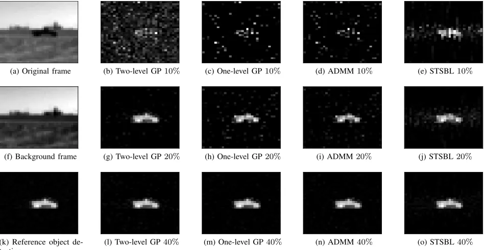
Fig. 7 presents the reconstructed sample frame from the Convoy data. For all the algorithms, the reconstruction results are provided for the undersampling ratio 10%, where the proposed algorithms slightly underperform the competitors in terms of the quality metrics, for the undersampling ratio 20%, where the proposed algorithm outperforms the competitors both in terms of NMSE and the F-measure, and for the undersampling ratio 40%, where the proposed algorithms show a little higher NMSE. It is clearly seen that for the undersampling ratio10%the difference in the quality metrics is insignificant since none of the methods is able to reconstruct the signal. The STSBL represents an exceptional example but still the frame reconstructed by this method contains considerable
amount of noise. For the undersampling ratio20%the proposed method provides the clear reconstructed frame in contrast to the reconstructed frames by all the competitors that are more noisy. Meanwhile, for the undersampling ratio 40% the difference between reconstruction results by all four algorithms is not remarkable.
Note that similar to the synthetic data experiment the proposed algorithms obtain the best results for the lowest un-dersampling ratio values where the reconstruction is reasonable, i.e. they require a less number of observations.
C. Real data: EEG source localisation
The third experiment is devoted to the EEG source localisa-tion problem.
The goal of the non-invasive EEG source localisation problem is to find 3D locations of dipoles such that their electromagnetic field coincides with the field measured by electrodes on the human head cortex. This is important, for example, for localisation of active areas in human-brain interfaces and treatment of neurological disorders [41], [42]. This problem is ill-posed in sense that there exist an infinite number of possible active areas inside the brain that could produce the same field on the head cortex. To regularise the problem, we use the idea that slab locations are distributed in space and temporally evolve, similar to [43]. Similar idea applies to the MEG source localisation [44].
Using the earlier introduced notation, the EEG source localisation problem is stated as
yt=Axt+εt, ∀t∈[1,. . . , T], (35)
where yt ∈ RK is the vector containing observations of
potential differences taken from K = 69 electrodes placed on a human head cortex,A∈RK×N is the lead field matrix corresponding toN/3 = 272 voxels, xt∈RN is the signal, that is the current density of dipole activation.
Herextrepresents the dipole moments corresponding to the grid locations:
xt=hx1x, x1y, x1z, x2x, x2y, x2z, . . . , xN 3z
i⊤
. (36)
For each grid voxel i inside the brain with location coordi-nates loc(i) = (xi, yi, zi) the corresponding dipole moments
(xix, xiy, xiz)along the 3D axis are considered.
We employ the following covariance function that promotes close values for collinear dipole moments corresponding to close grid positions
K(i, j) =αKexp
−d(i, j) 2
2ℓ2
K
, K∈ {Σ0,W}, (37)
where the distance is computed as
d(i, j) = (
0,if axis for dipole momentsi,j are different
||loc(i)−loc(j)||2
2,otherwise.
(38) Hyperparameters are selected so that the sampled potential differences have the similar behaviour as the provided data.
(a) Original frame (b) Two-level GP10% (c) One-level GP10% (d) ADMM10% (e) STSBL10%
(f) Background frame (g) Two-level GP20% (h) One-level GP20% (i) ADMM20% (j) STSBL20%
(k) Reference object de-tection
[image:11.612.68.542.65.310.2](l) Two-level GP40% (m) One-level GP40% (n) ADMM40% (o) STSBL40%
Fig. 7. Sample frame with reconstruction results from sparse observations for the Convoy data. (a), (f): the original and static background non-compressed frames; (k): object detection results based on non-compressed frame difference (static background frame is subtracted from the original frame); (b), (g), (l): reconstruction of compressed object detection results based on the proposed online two-level GP method; (c), (h), (m): reconstruction of the compressed object detection results based on the one-level GP method; (d), (i), (n): reconstruction of the compressed object detection results based on the ADMM method; (e), (j), (o): reconstruction of the compressed object detection results based on the STSBL method. (b), (c), (d), and (e) show the results for the undersampling rate10%, where all the algorithms fail to reconstruct the true signal. (g), (h), (i), and (j) show the reconstruction for the undersampling rate20%, where the difference in performance between the algorithms is visible. While for the undersampling rate40%((l), (m), (n), and (o)) reconstruction results are indistinguishable in quality.
(a) Located dipole moments 1 ms after the event
[image:11.612.56.293.422.544.2](b) Located dipole moments 170 ms after the event
Fig. 8. Located dipoles by the proposed offline two-level GP method for the EEG source localisation problem. There is no brain response immediately after the event and (a) demonstrates reconstructed brain active area that remains active during the whole period and it is not related to the event. While (b) shows the reconstructed active area when the brain response to the event is detected.
EEGLAB for the source localisation problem with annotated events.
Figure 8 presents located dipoles by the proposed method for the fourth event at two given time moments. The first time moment is taken right after the event happened and there is no response to it in the brain activity yet. The second time moment is chosen when the response is detected. Figure 9 shows the comparison of measured and restored potential differences by the proposed algorithm.
The true signalXis unknown for the EEG source localisation
Measured EEG
50 100 150 200 250
10
20
30
40
50
60
-0.4 -0.3 -0.2 -0.1 0 0.1 0.2 0.3 0.4
(a) Measured EEG
Restored EEG
50 100 150 200 250
10
20
30
40
50
60
-0.4 -0.3 -0.2 -0.1 0 0.1 0.2 0.3 0.4
[image:11.612.312.563.424.537.2](b) Reconstructed EEG (AXˆ) Fig. 9. Reconstruction by the proposed offline two-level GP method of the EEG signal. As the true active dipole areas are not known, reconstruction quality is based on the observationsY. Reconstructed EEG has lower magnitude, potentially because noise has been taken into account.
problem, therefore, NMSE between the observations yt and
reconstructedAxbt is used for the quantitative comparison in
165 170 175 0.2
0.25 0.3 0.35
time
NMSE
Two-level GP Two-level GP online One-level GP approx
[image:12.612.95.256.266.359.2]ADMM
Fig. 10. Results for NMSE betweenytandAxbtduring the brain response
time. The proposed algorithms referred as two-level GP and two-level GP online have the lowest NMSE among the others.
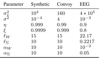
TABLE I
TWO-LEVELGPHYPERPARAMETERS
Parameter Synthetic Convoy EEG
σ2
x 104 160 4∗105
σ2 10−4 4 10−3
η 0.999 0.99 0.9
ξ 0.9999 0.999 0.8
ℓW 15 15 22.17
ℓΣ 10 10 0.2217
αW 10 10 10−2
αΣ 10 10 0.05
D. Parameters selection
For the proposed algorithm and for the one-level GP the parametersη andξare grid optimised to make the comparison fair. The prior shape hyperparameters ℓΣ,ℓW, αΣ, αW and
variancesσ2
x andσ2are specified so that sampled data has the
same form as training data. ADMM and STSBL use the default values of parameters. The selected hyperparameter values for the proposed algorithm for all datasets are presented in Table I.
VII. CONCLUSIONS
This paper proposes a new hierarchical Gaussian process model of spatio-temporal structure representation with complex temporal evolution in sparse Bayesian inference methods. This is achieved using the flexible hierarchical GP prior for the spike and slab model, where spatial and temporal structural dependencies are encoded by different levels of the prior. Offline and online methods are developed for posterior inference for this model.
We show that the introduced model can be applied to different areas such as compressive sensing and EEG source localisation. The results show the superiority of the proposed method in comparison with the non-hierarchical GP method, the alternating direction method of multipliers and the spatio-temporal sparse Bayesian learning method. The developed algorithms demonstrate better performance both in terms of signal value reconstruction and localisation of non-zero signal components: within the low amount of measurements range it achieves around 15% improvement in terms of slab localisation quality.
Acknowledgments: The authors would like to thank the support from the EC Seventh Framework Programme [FP7 2013-2017] TRAcking in compleX sensor systems (TRAX) Grant agreement no.: 607400.
REFERENCES
[1] M. F. Duarte and Y. C. Eldar, “Structured compressed sensing: From theory to applications,”IEEE Transactions on Signal Processing, vol. 59, no. 9, pp. 4053–4085, 2011.
[2] I. F. Gorodnitsky and B. D. Rao, “Sparse signal reconstruction from limited data using FOCUSS: A re-weighted minimum norm algorithm,”
IEEE Transactions on Signal Processing, vol. 45, no. 3, pp. 600–616, 1997.
[3] J. Yin and T. Chen, “Direction-of-arrival estimation using a sparse representation of array covariance vectors,”IEEE Transactions on Signal Processing, vol. 59, no. 9, pp. 4489–4493, 2011.
[4] R. Tibshirani, “Regression shrinkage and selection via the lasso,”Journal of the Royal Statistical Society. Series B (Methodological), vol. 58, no. 1, pp. 267–288, 1996.
[5] D. Malioutov, M. Çetin, and A. S. Willsky, “A sparse signal reconstruction perspective for source localization with sensor arrays,”IEEE Transactions on Signal Processing, vol. 53, no. 8, pp. 3010–3022, 2005.
[6] A. Carmi, P. Gurfil, and D. Kanevsky, “Methods for sparse signal recovery using Kalman filtering with embedded pseudo-measurement norms and quasi-norms,”IEEE Transactions on Signal Processing, vol. 58, no. 4, pp. 2405–2409, 2010.
[7] E. J. Candes and T. Tao, “Decoding by linear programming,”IEEE Transactions on Information Theory, vol. 51, no. 12, pp. 4203–4215, 2005.
[8] A. M. Tillmann and M. E. Pfetsch, “The computational complexity of the restricted isometry property, the nullspace property, and related concepts in compressed sensing,” IEEE Transactions on Information Theory, vol. 60, no. 2, pp. 1248–1259, 2014.
[9] M. E. Tipping, “Sparse Bayesian learning and the relevance vector machine,”The Journal of Machine Learning Research, vol. 1, pp. 211– 244, 2001.
[10] S. Mohamed, K. Heller, and Z. Ghahramani, “Bayesian and L1 approaches to sparse unsupervised learning,” inProceedings of the 29th International Conference on Machine Learning, 2012, pp. 751–758.
[11] T. J. Mitchell and J. J. Beauchamp, “Bayesian variable selection in linear regression,”Journal of the American Statistical Association, vol. 83, no. 404, pp. 1023–1032, 1988.
[12] N. G. Polson and J. G. Scott, “Shrink globally, act locally: Sparse Bayesian regularization and prediction,”Bayesian Statistics, vol. 9, pp. 501–538, 2010.
[13] K. P. Murphy,Machine learning: a probabilistic perspective. MIT press, 2012.
[14] F. Bach, R. Jenatton, J. Mairal, G. Obozinskiet al., “Structured sparsity through convex optimization,” Statistical Science, vol. 27, no. 4, pp. 450–468, 2012.
[15] S. Mallat,A wavelet tour of signal processing, third edition: the sparse way, 3rd ed. Academic Press, 2008.
[16] T. Hastie, R. Tibshirani, and M. Wainwright,Statistical learning with sparsity: the lasso and generalizations. CRC Press, 2015.
[17] J. Yang, X. Yuan, X. Liao, P. Llull, D. Brady, G. Sapiro, and L. Carin, “Video compressive sensing using Gaussian mixture models,”IEEE Transactions on Image Processing, vol. 23, no. 11, pp. 4863–4878, 2014.
[18] M. Yuan and Y. Lin, “Model selection and estimation in regression with grouped variables,”Journal of the Royal Statistical Society: Series B (Statistical Methodology), vol. 68, no. 1, pp. 49–67, 2006.
[19] P. Sprechmann, I. Ramirez, G. Sapiro, and Y. C. Eldar, “C-HiLasso: A col-laborative hierarchical sparse modeling framework,”IEEE Transactions on Signal Processing, vol. 59, no. 9, pp. 4183–4198, 2011.
[20] A. Schmolck, “Smooth relevance vector machines,” Ph.D. dissertation, University of Exeter, 2008.
[21] M. A. Van Gerven, B. Cseke, F. P. De Lange, and T. Heskes, “Efficient Bayesian multivariate fMRI analysis using a sparsifying spatio-temporal prior,”NeuroImage, vol. 50, no. 1, pp. 150–161, 2010.
[22] A. Wu, M. Park, O. O. Koyejo, and J. W. Pillow, “Sparse Bayesian structure learning with dependent relevance determination priors,” in
[23] W. Chen, D. Wipf, Y. Wang, Y. Liu, and I. J. Wassell, “Simultaneous Bayesian sparse approximation with structured sparse models,”IEEE Transactions on Signal Processing, vol. 64, no. 23, pp. 6145–6159, 2016. [24] Z. Zhang and B. D. Rao, “Sparse signal recovery with temporally correlated source vectors using sparse Bayesian learning,”IEEE Journal of Selected Topics in Signal Processing, vol. 5, no. 5, pp. 912–926, 2011. [25] M. R. Andersen, A. Vehtari, O. Winther, and L. K. Hansen, “Bayesian inference for spatio-temporal spike and slab priors,”arXiv preprint arXiv:1509.04752, 2015.
[26] M. Deisenroth and S. Mohamed, “Expectation propagation in Gaus-sian process dynamical systems,” inAdvances in Neural Information Processing Systems, 2012, pp. 2609–2617.
[27] N. D. Lawrence and A. J. Moore, “Hierarchical Gaussian process latent variable models,” inProceedings of the 24th International Conference on Machine learning, 2007, pp. 481–488.
[28] M. J. Wainwright and M. I. Jordan, “Graphical models, exponential families, and variational inference,”Foundations and Trends in Machine Learning, vol. 1, no. 1–2, pp. 1–305, 2008.
[29] E. I. George and R. E. McCulloch, “Variable selection via Gibbs sampling,” Journal of the American Statistical Association, vol. 88, no. 423, pp. 881–889, 1993.
[30] B. E. Engelhardt and R. P. Adams, “Bayesian structured sparsity from Gaussian fields,”ArXiv e-prints, 2014.
[31] Q. Wu, Y. D. Zhang, M. G. Amin, and B. Himed, “High-resolution passive SAR imaging exploiting structured Bayesian compressive sensing,”IEEE Journal of Selected Topics in Signal Processing, vol. 9, no. 8, pp. 1484– 1497, 2015.
[32] C. E. Rasmussen and C. K. I. Williams,Gaussian processes for machine learning. The MIT Press, 2006.
[33] T. P. Minka, “Expectation propagation for approximate Bayesian infer-ence,” inProceedings of the 17th Conference on Uncertainty in Artificial Intelligence, 2001, pp. 362–369.
[34] J. M. Hernandez-Lobato, D. Hernandez-Lobato, and A. Suarez, “Expec-tation propagation in linear regression models with spike-and-slab priors,”
Machine Learning, vol. 99, no. 3, pp. 437–487, 2015.
[35] T. Minka and J. Lafferty, “Expectation-propagation for the generative aspect model,” inProceedings of the 18th Conference on Uncertainty in Artificial Intelligence, 2002, pp. 352–359.
[36] S. Boyd, N. Parikh, E. Chu, B. Peleato, and J. Eckstein, “Distributed optimization and statistical learning via the alternating direction method of multipliers,”Foundations and Trends in Machine Learning, vol. 3, no. 1, pp. 1–122, 2011.
[37] Z. Zhang, T.-P. Jung, S. Makeig, Z. Pi, and B. D. Rao, “Spatiotemporal sparse Bayesian learning with applications to compressed sensing of multichannel physiological signals,”IEEE Transactions on Neural Systems and Rehabilitation Engineering, vol. 22, no. 6, pp. 1186–1197, 2014.
[38] B. Xin, Y. Wang, W. Gao, D. Wipf, and B. Wang, “Maximal sparsity with deep networks?” inAdvances in Neural Information Processing Systems, 2016, pp. 4340–4348.
[39] G. Warnell, S. Bhattacharya, R. Chellappa, and T. Basar, “Adaptive-rate compressive sensing using side information,”IEEE Transactions on Image Processing, vol. 24, no. 11, pp. 3846–3857, 2015.
[40] V. Cevher, A. Sankaranarayanan, M. F. Duarte, D. Reddy, and R. G. Baraniuk, “Compressive sensing for background subtraction,” in Pro-ceedings of 10th European Conference on Computer Vision, 2008, pp. 155–168.
[41] M. A. Jatoi, N. Kamel, A. S. Malik, I. Faye, and T. Begum, “A survey of methods used for source localization using EEG signals,”Biomedical Signal Processing and Control, vol. 11, pp. 42–52, 2014.
[42] S. Baillet, J. C. Mosher, and R. M. Leahy, “Electromagnetic brain mapping,”IEEE Signal Processing Magazine, vol. 18, no. 6, pp. 14–30, 2001.
[43] S. Baillet and L. Garnero, “A Bayesian approach to introducing anatomo-functional priors in the EEG/MEG inverse problem,”IEEE Transactions on Biomedical Engineering, vol. 44, no. 5, pp. 374–385, 1997. [44] A. Solin, P. Jylänki, J. Kauramäki, T. Heskes, M. A. van Gerven,
and S. Särkkä, “Regularizing solutions to the MEG inverse prob-lem using space-time separable covariance functions,”arXiv preprint arXiv:1604.04931, 2016.
[45] A. Delorme and S. Makeig, “EEGLAB: an open source toolbox for analysis of single-trial EEG dynamics including independent component analysis,”Journal of Neuroscience Methods, vol. 134, no. 1, pp. 9–21, 2004.
APPENDIXA
PRODUCT AND QUOTIENT RULES
EP updates are based on products and quotients of distribu-tions. This section presents the product and quotient rules for Gaussian and Bernoulli distributions.
A. Product of Gaussians
A product of two Gaussian distributions is a unnormalised Gaussian distribution
N(x;m1,Σ1)N(x;m2,Σ2)∝ N(x;m,Σ),
where
Σ−1=Σ−11+Σ−21,Σ−1m=Σ−11m1+Σ−21m2
B. Quotient of Gaussians
A quotient of two Gaussian distributions is a unnormalised Gaussian distribution3
N(x;m1,Σ1) N(x;m2,Σ2)
∝ N(x;m,Σ),
where
Σ−1=Σ−11−Σ−21,Σ−1m=Σ−11m1−Σ−21m2
C. Product of Bernoulli
A product of two Bernoulli distributions is a unnormalised Bernoulli distribution
Ber(x; Φ(z1))Ber(x; Φ(z2))∝Ber(x; Φ(t(z1, z2))),
where
t(z1, z2) = Φ−1
(1−Φ(z1))(1−Φ(z2))
Φ(z1)Φ(z2)
+ 1 −1!
D. Quotient of Bernoulli
A quotient of two Bernoulli distributions is a unnormalised Bernoulli distribution
Ber(x; Φ(z1))
Ber(x; Φ(z2))
∝Ber(x; Φ(d(z1, z2))),
where
d(z1, z2) = Φ−1 (1
−Φ(z1))Φ(z2)
(1−Φ(z2))Φ(z1)
+ 1 −1!
3Although quotient can lose positive semidefiniteness, we will still refer to
APPENDIXB EP UPDATE FOR FACTORfit
A. Cavity distribution
The unnormalised cavity distribution q\qfit(x
it, ωit) = q(xit,ωit)
qfit(xit,ωit) can be computed as
q\qfit = N(xit;mt(i),Vt(i, i))Ber(ωit; Φ(zit))
N(xit;mft(i),Vft(i, i))Ber(ωit; Φ(zfit)) ∝ N(xit;m
\f it, v
\f
it)Ber(ωit; Φ(z
\f it )),
where
(vit\f)−1=V−1
t (i, i)−V
−1
ft (i, i),
(vit\f)−1mit\f =Vt−1(i, i)mt(i)−V−ft1(i, i)mft(i, i),
zit\f =zhit
B. Moments matching
The moments of the tilted distribution q\qfitf itare
Zit= Φ(zit\f)N(0;m
\f it, v
\f it)
+ (1−Φ(zit\f))N(0;m\itf, v\itf+σ2
x),
Exit=
1−Φ(zit\f)
Zit
N(0;m\itf, vit\f) m
\f itσx2
v\itf+σ2
x
,
Ex2
it=
1−Φ(zit\f)
Zit
N(0;m\itf, vit\f)
× (m
\f it)2σx4
(v\itf+σ2
x)2
+ v
\f it σx2
vit\f+σ2
x
!
,
Eωit=
Φ(zit\f)
Zit
N(0;m\itf, v\itf)
The new approximation q∗(x
it, ωit)is
q∗=N(xit;mq
∗
it, v q∗
it)Ber(ωit; Φ(zq
∗
it)),
where
mqit∗ =Exit, vq
∗
it =Ex
2
it−(Exit)2, zq
∗
it = Φ
−1(
Eωit).
C. Factor update
The new factor approximationqnew
fit(xit, ωit) =
q∗(xit,ωit)
q\qfit(xit,ωit)
can be computed as
qfnewit =
Nxit;mq
∗
it, v q∗ it
Ber
ωit; Φ
zqit∗
Nxit;m\itf, v
\f it
Berωit; Φ
zit\f
∝ N xit;mnewft (i),V
new
ft (i, i)
Ber ωit; Φ zfnewit
,
where
Vnewft −1(i, i) =vitq∗−1−vit\f−1,
Vnewf it
−1
(i, i)mnewf
t (i) =
vitq∗−1mqit∗−v\itf−1m\fitf,
znew
fit =d
zitq∗, zit\f.
APPENDIXC EP UPDATE FOR FACTORhit
A. Cavity distribution
The unnormalised cavity distribution q\qhit(γ
it, ωit) = q(γit,ωit)
qhit(γit,ωit) can be computed as
q\qhit = N(γit;νt(i),S(i, i))Ber(ωit; Φ(zit)) N(γit;νht(i),Sh(i, i))Ber(ωit; Φ(zhit)) ∝ N(γit;ν
\h
it, s
\h
it)Ber(ωit; Φ(z
\h
it )),
where
(s\ith)−1=St−1(i, i)−S−h1(i, i)
(s\ith)−1νit\h=S−t1(i, i)µt(i)−Sh−1(i, i)νht(i, i)
zit\h=zfit
B. Moments matching
The moments of the tilted distributionq\qhith it are
Zit= Φ(z
\h
it)Φ(a) + (1−Φ(z
\h
it))(1−Φ(a)),
Eγit=
1
Zit
(Φ(z\ith)K+ (1−Φ(zit\h))(νit\h−K)),
Eγ2it= 1
Zit
(2Φ(zit\h)−1)
(νit\h)2Φ(a) +s\ithΦ(a)
+2ν
\h
it s
\h
itN(a; 0,1)
q 1 +s\ith
−(s
\h
it)2aN(a; 0,1)
1 +s\ith
+ (1−Φ(zit\h)(sit\h+ (νit\h)2)
,
Eωit=
Φ(zit\h)Φ(a)
Zit
,
where
a= ν
\h
it
q 1 +s\ith
, K=s\ithNq(a; 0,1) 1 +s\ith
+νit\hΦ(a)
The new approximation q∗(γ
it, ωit)is
q∗=N(γit;νq
∗
it, s q∗
it)Ber(ωit; Φ(zq
∗
it)),
where
νitq∗ =Eγit, sq
∗
it =Eγ
2
it−(Eγit)2, zq
∗
it = Φ
−1(
Eωit).
C. Factor update
The new factor approximation qnew
hit(γit, ωit) = q∗(γ
it, ωit)
q\qhit(γ it, ωit)
can be computed as
qnew
hit =
Nγit;νq
∗
it, s q∗ it
Ber
ωit; Φ
zitq∗
Nγit;ν\ith, s
\h
it
Berωit; Φ
zit\h
∝ N γit;νnewht (i),S
new
h (i, i)
Ber ωit; Φ zhnewit
,
where
(Snewh )−1(i, i)νnew
ht (i) =
sqit∗−1νitq∗−s\ith−1νit\h,
znew
hit =d
zitq∗, z\ith.
APPENDIXD EP UPDATE FOR FACTORrt
A. Cavity distribution
The unnormalised cavity distribution q\qrt(γ
t,µt) = q(γt,µt)
qrt(γt,µt) can be computed as
q\qrt = N(γt;νt,S)N(µt;et,D)
N(γt;νrt,Sr)N(µt;ert,Dr) ∝ N(γt;ν\tr,S\r)N(µt;e\tr,D\r),
where
(S\r)−1= (S)−1−(Sr)−1
(S\r)−1ν\tr= (S)−1νt−(Sr)−1νrt
(D\r)−1= (D)−1−(Dr)−1
(D\r)−1e\tr= (D)−1et−(Dr)−1ert
B. Find the update for the factor qnew
rt
For the factorqrt parameters of the Gaussian distributions
found during the moment matching step are cancelled out during the factor update step and the resulting formulae are
qnew
rt (γt,µt)∝ N γt;ν
new
rt ,S
new
r
N µt;enewrt ,Dnewr ,
where
Snewr =D\r+Σ0, νnewrt =e
\r t
Dnewr =S\r+Σ0, enewrt =ν
\r t .
APPENDIXE EP UPDATE FOR FACTORut
A. Cavity distribution
The unnormalised cavity distribution q\qut(µ
t−1,µt) =
q(µt−1,µt)
qut(µt−1,µt)
can be computed as
q\qut = N(µt−1;et−1,D)N(µt;et,D) N(µt−1;eut←,Du←)N(µt;eut→,Du→)
∝ N(µt−1;e
\u
t−1,D
\u
t−1)N(µt;e
\u
t ,D
\u
t ),
where
(D\t−u1)−1= (D)−1−(Du←)−1
(D\t−u1)−1e\t−u1= (D)−1et−1−(Du←)−1eut←
(D\tu)−1= (D)−1−(Du→)−1
(D\tu)−1e\tu= (D)−1et−(Du→)−1eut→
B. Find the update for the factor qnew
ut
For the factorqut parameters of the Gaussian distributions
found during the moment matching step are cancelled out during the factor update step and the resulting formulae are
qnew
ut (µt−1,µt)∝ N µt;e
new
ut→,D
new
u→
N µt−1;enewut←,D
new
u←
,
where
Dnewu→=D\t−u1+W, enewut→=e\t−u1 Dnewu←=D\tu+W, enewu
t←=e
\u