Evaluation of the diffusion equation for modeling reverberant electromagnetic fields

electromagnetic fields

.

White Rose Research Online URL for this paper:

http://eprints.whiterose.ac.uk/106570/

Version: Accepted Version

Article:

Flintoft, Ian David orcid.org/0000-0003-3153-8447, Marvin, Andrew Charles

orcid.org/0000-0003-2590-5335, Funn, Foo Inn et al. (4 more authors) (2017) Evaluation

of the diffusion equation for modeling reverberant electromagnetic fields. IEEE

Transactions on Electromagnetic Compatibility. pp. 760-769. ISSN 0018-9375

https://doi.org/10.1109/TEMC.2016.2623356

[email protected] https://eprints.whiterose.ac.uk/ Reuse

Items deposited in White Rose Research Online are protected by copyright, with all rights reserved unless indicated otherwise. They may be downloaded and/or printed for private study, or other acts as permitted by national copyright laws. The publisher or other rights holders may allow further reproduction and re-use of the full text version. This is indicated by the licence information on the White Rose Research Online record for the item.

Takedown

If you consider content in White Rose Research Online to be in breach of UK law, please notify us by

Author post-print

Evaluation of the Diffusion Equation for Modeling Reverberant Electromagnetic

Fields

Ian D. Flintoft

_{, Andy C. Marvin}

_{, Foo Inn Funn}

_{, Linda Dawson}

_{, Xiaotian Zhang}

_{, Martin P. Robinson}

and John. F. Dawson

1_{Department of Electronics, University of York, Heslington, York YO10 5DD, UK} 2_{Republic of Singapore Airforce, Singapore}

Published in IEEE Transaction on Electromagnetic Compatibility

Accepted for publication 23/10/2016

DOI:

10.1109/TEMC.2016.2623356



Abstract—_{Determination of the distribution of electromagnetic} energy inside electrically large enclosed spaces is important in many electromagnetic compatibility applications, such as certification of aircraft and equipment shielding enclosures. The field inside such enclosed environments contains a dominant diffuse component due to multiple randomizing reflections from the enclosing surfaces. The power balance technique has been widely applied to the analysis of such problems; however, it is unable to account for the inhomogeneities in the field that arise when the absorption in the walls and contents of the enclosure is significant. In this paper we show how a diffusion equation approach can be applied to modeling diffuse electromagnetic fields and evaluate its potential for use in electromagnetic compatibility applications. Two canonical examples were investigated: A loaded cavity and two cavities coupled by a large aperture. The predictions of the diffusion model were compared to measurement data and found to be in good agreement. The diffusion model has a very low computational cost compared to other applicable techniques, such as full-wave simulation and ray-tracing, offering the potential for a radical increase in the efficiency of the solution high frequency electromagnetic shielding problems with complex topologies.

Index Terms— _{asymptotic techniques, power balance,} absorption cross-section, reverberation chamber, shielding

I. INTRODUCTION

he statistical energy or power balance (PWB) approach to analyzing the average electromagnetic (EM) field inside electrically large cavities has been used for many years by the electromagnetic compatibility (EMC) community. It is the foundation of reverberation chamber (RC) theory [1], [2] and is also widely used for first order estimates in high frequency shielding problems [3] and estimating environmental electromagnetic exposure [4]. The PWB model assumes that the degrees of freedom in the EM field are completely diffused by reflections from the cavity walls (and contents if present) leading to well defined statistical distribution

Submitted for review 22th _{July 2016. Accepted for publication 23}rd _October 2016.

I. D. Flintoft, A. C. Marvin, X. Zhang, L. Dawson, M. P. Robinson and J. F. Dawson are with the Department of Electronics, University of York, Heslington, York, YO10 5DD (e-mail: [email protected],

[email protected], [email protected], [email protected],

[email protected]).

Foo Inn Funn is with the Republic of Singapore Airforce, having completed a MEng degree in the Department of Electronics, University of York, UK (email: [email protected]).

functions for the fields and homogeneous and isotropic average values related to the losses (both dissipative and via apertures) in the cavity.

A fundamental limitation of the PWB model is that it cannot account for the inhomogeneity in the diffuse field arising from any loss in the cavity. If the distribution of loss is itself non-uniform this will drive even greater inhomogeneity in the diffuse field. When the losses are small this may not be a significant limitation since the multiple scatterings from the walls mean that the diffuse EM field is still highly uniform and isotropic. However, for moderate loss, where there are still sufficient scatterings for an approximately diffuse field to be established, the PWB model becomes inaccurate.

This limitation is important in a number of EMC applications. In RCs the spatial and angular anisotropy of the plane-wave spectrum is often ascribed to the presence of non-stochastic direct paths as defined by the ‘K-factor’ [5], [6]. For measurements made in RCs with significant loading, for example, when measuring absorption cross-section (ACS) [7] or using loading to replicate multipath environments [8], the absorption also induces inhomogeneity and therefore contributes to the systematic error. This error is often treated on a statistical basis, for example, by measuring the average field at a number of locations in the working volume and characterizing the non-uniformity (proximity effect) from the deviation of these samples [9].

The acoustics community has developed a diffusion equation based model that can account for the variation of the diffuse energy density in enclosed spaces due to the presence and distribution of losses on the walls and contents of the enclosure. Recent reviews of this acoustic diffusion model (ADM) are given in [10], [11].

The purpose of this paper is to make an initial evaluation of the diffusion equation model for EMC applications. In Section II we review the basic diffusion model developed in the acoustics literature and place it in the electromagnetic context. A dimensional reduction technique that can be used to derive two-dimensional approximations for simple geometries is described in Section III and its finite element method solution is outlined. In Section IV we present the solution of two canonical examples relevant to EMC applications; validation measurements for the examples are then described in Section V. We conclude in Section VI.

Evaluation of the Diffusion Equation for

Modeling Reverberant Electromagnetic Fields

Ian D. Flintoft,

Senior Member, IEEE

, Andy C. Marvin,

Fellow, IEEE

, Foo Inn Funn, Linda Dawson,

Xiaotian Zhang, Martin P. Robinson,

Member, IEEE

and John. F. Dawson,

Member, IEEE

Author post-print 2

II. THE DIFFUSION MODEL

A. Statement of the diffusion model

The diffusion model can be derived from a radiative

transport theory of “particles” (analogous to EM rays) in a cavity [12]. It assumes the existence of a diffuse EM field with average energy density [2], where denotes an average over a statistical ensemble of systems, for example, mode tuning configurations in an RC. The basic assumptions of the model, put into the context of electromagnetics are:

1. Geometric optics: The rays propagate according to geometric optics (GO), requiring that the wavelength is small compared to the size of the cavity and scattering objects within it;

2. Diffuse scattering: Seen over the statistical averaging ensemble (e.g. mode tuning configurations in an RC) the scattering randomizes the ray directions;

3. Directional broadening: On average reflection dominates over absorption, so after multiple reflections the diffuse field is driven towards being isotropic; 4. Temporal broadening: The time-scale for changes in

the diffuse energy density is long compared to the mean-free-time between scattering events.

The electromagnetic wavelength, , only enters the model via the frequency dependence of the absorption processes within the cavity. The diffusion process itself is governed by a frequency independent diffusivity (diffusion coefficient) primarily determined by the geometry of the cavity. The vector nature of the electromagnetic field also only appears implicitly within the absorption and scattering efficiencies of the cavity and its contents. This electromagnetic diffusion model (EDM) is a generalization of the PWB approach; in Section II.D we demonstrate that both frequency-domain and time-domain PWB methods are special cases of the EDM.

Within the assumptions outlined above the diffuse electromagnetic energy density within the volume of an enclosed space, V, satisfies a diffusion equation [13]

(1) where is the diffusivity, is a volumetric energy loss rate due to absorption in the cavity contents and we have assumed there is a time-dependent isotropic point source of total radiated power located at . On the boundary surface of the volume, , the energy density is assumed to satisfy a Robin flux type boundary condition (BC)

c (2)

where c is the speed of light, is an outward unit normal vector and is an absorption factor related to the average reflection coefficient of the walls.

The diffusivity is related to the overall mean-free-path (MFP), , between scatterings of the rays from the walls and contents of the cavity by [14]

c (3)

where the MFP for scattering from the walls is given by [13]

. (4)

If we assume the contents are a set of identical objects

with average scattering cross-section then the MFP for scattering from them is [15]

(5)

At high frequencies the average scattering cross-section can be estimated as , where is the surface area of the scattering objects. The dependence of the MFP on the chamber volume and surface area of the objects can be understood intuitively from the image theory of the cavity [16]; if is small a ray will scatter off the walls many times before intercepting the scatterer and the MFP will be much larger than the chamber size. The overall MFP is determined by the harmonic mean [15]

(6) The simplest estimate of the absorption factor for the walls corresponds to Sabine’s formula in acoustics [17],

(7)

where is the average absorption efficiency. For the EDM this can be determined using the standard estimate of wall losses in a reverberation chamber,

cos (8) where are the Fresnel reflection coefficients for transverse electric and magnetic fields at angle of incidence from the normal to the wall [18]. This absorption model assumes the diffused rays undergo specular reflections from the walls and is the route by which the electromagnetic frequency and polarization enter into the EDM.

For high wall absorption efficiencies, , alternative models have been found to be more accurate in room acoustics [19], [20], [21]; some of these have recently been investigated for room electromagnetics applications and found to have similar validity for electromagnetic reverberation [22]. The radiative transport derivation of the diffusion model leads to the expression

(9)

for the absorption factor [19]. This model assumes the reflection at the walls is completely diffuse, i.e. the power reflectance is independent of the angle of incidence. For low absorption it predicts a loss factor that is close to that of the Sabine formula above; however, for high absorption the loss factor approaches twice that of Sabine’s formula.

The energy loss rate from absorption in the contents is [23]

c (10)

where is the average absorption efficiency of the objects. The flux of the diffuse energy density in the cavity is given

by Fick’s Law [24]

(11) A non-zero flux of energy density must be present in any cavity with loss in order to transport the energy from the source to the absorption points. This flux is therefore related to the anisotropy of the diffuse field induced by the presence of absorption in the cavity.

B. Sources

single point source is assumed. The time independent Green’s function for the diffusion equation in an unbounded space is given by [24]

exp (12)

This includes a spurious “direct” term,

, close to the source, . It arises from the fact that near the source a diffuse field has not been established and the diffusion equation is therefore unable to correctly describe the physical inverse square law variation of the direct energy density. Visentin et al [24] argue that this spurious term should be subtracted from the solution to give the true reverberant energy density

, (13)

with the physical direct energy from the source being

determined using c This is

supported experimentally in acoustics for cavities without a strong aspect ratio. The spurious effect can also be mitigated by smearing the source out over a volume of space or using surface sources [23]. In this paper we have not applied the correction in (13) so the energy density and derived quantities within about 50 mm of the source antenna should be disregarded when considering the results.

C. Coupled cavities

Two cavities coupled through an electrically large aperture can be treated as a single computational domain in the EDM, with no special treatment of the aperture. This method assumes that the field in the aperture is well diffused, which is only a good approximation for apertures well above their resonant frequency. Providing the coupling area is not too

large each cavity’s diffusivity and loss rate will be

approximately determined by its own respective geometry and absorption characteristics and unaffected by the coupling. If the coupling area is large then the diffusivity may need to be modified and could become inhomogeneous.

In order to accurately model apertures that are either electrically small or in the resonant regime a different approach is required. If we consider two coupled cavities with energy densities and such that part of their shared wall, is semi-transparent to the diffuse field, then on this part of the wall the BCs (2) are replaced by the coupled energy exchange BCs [25]

(14a)

(14b)

where is the average transmission efficiency of the wall and is its average absorption efficiency as seen from each side [26]. Here we have assumed that the transmission is reciprocal. For a lossless aperture and if is the aperture area then its average transmission cross-section in the high frequency limit is . The efficiency can then be used to account for the frequency dependence of the cross-section. In the high frequency limit and the transmission cross-section takes its GO limit value [1]. Note

that as defined here, the average transmission cross-section includes an extra factor of a half in order to account for the fact that the wall only sees half the scalar power density, c , coming from a half-space.

D. Energy balance

We now consider how the EDM relates to the PWB method. Integrating the diffusion equation over the volume of the cavity, applying Green’s theorem and then inserting the Robin BC on the cavity walls we obtain the general energy balance relationship [20]

c (16)

where the total energy in the cavity is

(17) First consider the case for a static and homogeneous energy density, . Further assuming the wall absorption is homogeneous and inserting the Sabine estimate (7) of the absorption factor and using (10) we obtain

c (18)

Identifying the scalar power density c and average absorption cross-sections of the walls, , and contents, , this is just the classic Hill et al PWB balance relationship [1]

(19) If we consider a homogeneous but time varying energy density (a situation that can only be an approximation to reality) then

(20) where c . This has solution

e e e d (21)

This time domain energy decay has been investigated in [28]. The diffusion approach is thus seen to be a natural generalization of the PWB technique that treats the distributed nature of the losses more accurately when the absorption is significant.

III. KANTOROVICH DIMENSIONAL REDUCTION

While the diffusion problem can be solved efficiently in three dimensions, for this initial evaluation we have adopted an even more efficient approach based on the dimensional reduction method of Kantorovich [29]. In this approach, for a cavity with a constant cross-sectional area normal to one direction, taken as the z-direction in this paper, that direction is eliminated from the problem by assuming an approximate solution that is separable:

(22) A typical ansatz for the variation in the z-direction is a quadratic, as would be obtained for a separable solution of the Laplace operator in a cuboid cavity. Note that we will take to be dimensionless in the following, so that carries the units J m-3 _{of energy density.}

Author post-print 4

by . This assumption is not necessary, but it considerably simplifies some of the relationships that follow. The Robin BCs on the lower and upper walls determine the unknown coefficients in the quadratic profile which can then be written

(23) where

c (24)

Note, if the lower and upper walls have non-zero absorption then cannot be constant since there must be an energy density gradient at those walls to support the absorbed power flux. Specializing to the steady-state case, it can then be shown using a variational residual minimization approach that the solution in the remaining directions satisfies a two-dimensional diffusion equation [30]

(25) with Robin BCs

c (26)

on the side walls. Here is the cross-sectional area of the cavity, is the curve defining the perimeter of this area and the other parameters are given by integrals over the vertical profile:

d (27)

d (28)

d (29)

d (30)

corresponds to an effective areal energy loss factor in the 2D model due to losses on the lower and upper surfaces.

Approximate solutions to some interesting practical problems can be determined very quickly from this reduced dimensionality formulation. In this paper the finite element method (FEM) was used to solve the reduced boundary value problem, implemented using FreeFEM++ [31]. The contents were modeled by including their surfaces in the mesh and applying a Robin BC, (2), with the appropriate loss factor. Coupled volumes were simulated using the energy exchange BCs in (14) implemented with an iterative algorithm. Note that in the EDM the mesh size is determined by the MFP and not by the electromagnetic wavelength; this allows a much coarser mesh to be used in the EDM than in full-wave simulation. All the FEM results in this paper were obtained in about one second on a desktop computer using triangular meshes with a typical mesh size of 30-40 mm.

IV. CANONICAL EXAMPLES

The two canonical examples investigated are based on the same geometry of a cuboid cavity occupying the volume

, and shown in Fig. 1. The walls are assumed to have a homogeneous absorption efficiency of and the cavity is excited by an isotropic source of total radiated power located at . An absorbing cylinder of radius and height can be positioned in the cavity, orientated with its axis in the z-direction, centered at The cylinder is assumed to have a homogeneous

absorption efficiency of .

The cavity can also be partitioned into two sub-cavities leaving a slot of width with the full height of the cavity located in the region , of the shared wall. The slot was chosen to span the whole cavity so that the dimensional reduction technique is applicable and it was located along the edge of the partition for experimental convenience in the validation measurements described in Section V.

The values of the parameters are given in Table I. The wall and cylinder absorption efficiencies were chosen to match those of the physical cavity and cylinder used for the validation measurements described in Section V.

A. Absorbing cylinder in a rectangular cavity

For Example A the partition in Fig. 1 is not present, leaving a single cavity loaded by an absorbing cylinder. Using the PWB approach, which assumes a homogeneous energy density, , we have from (18)

c (31)

where and . This

provides a reference level for comparison to the EDM results. The cavity was modeled using the approach detailed in Section III and the parameters in Table I, except where stated otherwise. For the FEM solution exactly reproduces the uniform energy density prediction of (31).

Fig. 2 shows the distribution of the energy density in the plane z for , normalized to the prediction of the PWB model,

(32)

which quantifies both the uniformity of the diffuse energy density and its deviation from the PWB estimate. This

Fig. 1. Cross-section of the cuboid cavity used for the canonical examples and validation measurements. For Example A the partition is not present, giving a single loaded cavity. For example B the partition is introduced to give two sub-cavities coupled by a slot. The small black dots represent the measurement locations in the plane used for the measurements.

TABLEI

PARAMETERS FOR THE CANONICAL EXAMPLES

Parameter Value Parameter Value

 0.45 m 0.01 m

0.45 m 0.225 m

d _{0.04 m 0.225 m}

0.05 m 1 W

0.0027 (Ex. A) 0.7 m 0.95 (Ex. B) 0.675 m

simulation uses the Sabine model (7) for the absorption factor. The absorption induces a non-uniformity of up to 3 dB in the energy density (ignoring the immediate vicinity of the source, since we have not subtracted the direct energy density term here) and the prediction of the PWB model is only valid over a limited spatial region; the maximum difference is about 1.5 dB in the right-hand half of the cavity.

At this point a brief discussion of the boundary fields in a cavity is pertinent. In a metallic cavity the fields within about half a wavelength of the walls must deviate from those of the ideal diffuse field in order to satisfy the electromagnetic boundary conditions at the surface of a good conductor [32]. Neither PWB nor the EDM directly account for this. However, for a low loss cavity the average energy density near the wall is the same as it is within the main volume of the cavity; it is just distributed differently between the electromagnetic field components, residing increasingly in the normal electric and tangential magnetic field components as the wall is approached. Since the EDM describes the average energy density it is therefore consistent with this boundary effect near the walls; it should however be borne in mind that this field anisotropy exists near highly conducting surfaces.

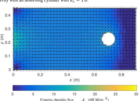
The flux of energy density necessary to sustain the

non-uniform distribution is given by Fick’s Law (11). Fig. 3 shows the energy density flux in the same plane for . The

transport of energy density from the source to the dominant absorption surface is clearly seen.

The uniformity of the scalar power density along the line down the center of the cavity is shown in Fig. 4 for a range of cylinder absorption efficiencies. The increasing inhomogeneity of the diffuse field with absorption efficiency of the cylinder is clearly apparent.

The non-uniformity and flux must clearly be associated with anisotropy in the plane-wave spectrum at each point in the cavity [2]: A net flow of energy in a given direction corresponds to more plane-waves propagating in that direction compared to the other directions. The diffusion model cannot determine this anisotropy in the plane-wave spectrum directly; however, the overall anisotropy can be estimated by comparing the magnitude of the energy density flow with the scalar power density at each point using the metric

(33)

Fig. 5 shows this metric for the case . Anisotropy of up to 1.3 dB is predicted close to the cylinder. A denser mesh was used for this simulation in order to capture the detailed variations.

Fig. 2. Diffuse energy density uniformity, (dB), in the cuboid cavity with an absorbing cylinder with .

Fig. 3. Diffuse energy density flux, , in the cuboid cavity with an absorbing cylinder with . The arrows indicate the direction of the flux while the color indicates the magnitude.

Fig. 4. Diffuse field scalar power density at along the line of the loaded cuboid cavity as a function of the cylinder’s average absorption efficiency comparing predictions of the diffusion model (lines with markers) to the standard power balance model (lines without markers).

Author post-print 6

B. Two cavities coupled by an aperture

In Example B we consider the coupling of the diffuse field between the two sub-cavities formed by introducing the partition in Fig. 1. We denoted the “source” sub-cavity

by “1” and the “coupled” sub-cavity by “2”. PWB analysis predicts that the energy densities in the two cavities,

and , are given by [33]

c , (34)

where are the absorption cross-sections of the two cavities, is the transmission

cross-section of the slot and . Here

is the total surface area of each sub-cavity. When cavity 2 is empty the solution in Fig. 6 is obtained for the parameters given in Table I. The uniformity is again defined as the ratio of the energy density to that predicted by the PWB in each sub-cavity (34). With this wall absorption efficiency, typical of a metallic enclosure, the inhomogeneity in the diffuse field is less than about 0.2 dB.

The variation of the scalar power density along a line through the cavity is shown in Fig. 7 for a range of wall absorption efficiencies. For the energy density is

relatively homogeneous and the difference from the PWB model is less than 0.1 dB. As increases the power density becomes more and more inhomogeneous; in particular, the power density in cavity 1 near the aperture falls below the PWB prediction. The spatial average energy density in the EDM deviates from the PWB model by 10 % for

and 30 % for .

The diffuse field uniformity in the coupled cavities when cavity 2 is loaded by an absorbing cylinder with

and the wall absorption efficiency is is shown in Fig. 8. The field in each cavity is again normalized to the PWB prediction. With the highly absorbing cylinder present in the second cavity the diffuse field varies by up to 3 dB from the PWB model estimate, with the greatest deviation near the aperture.

The variation of the power density along a line through the cavity is shown in Fig. 9 for a range of cylinder absorption efficiencies and wall absorption efficiency is . The spatial average energy density in the EDM deviates from the PWB model by 5 % for and 50 % for .

Fig. 6. Diffuse energy density uniformity, (dB), in unloaded coupled cuboid cavities with homogeneous wall absorption efficiency

.

Fig. 7. Diffuse field scalar power density in unloaded coupled cuboid cavities predicted by the diffusion model (lines with markers) compared to the standard power balance model (lines without markers) along the line

m.

Fig. 8. Diffuse energy density uniformity, (dB), in coupled cuboid cavities with homogeneous wall absorption efficiency

and absorbing cylinder with in cavity 2.

Fig. 9. Diffuse field scalar power density in loaded coupled cuboid cavities predicted by the diffusion model (lines with markers) compared to the standard power balance model (lines without markers) along the line

V. VALIDATION MEASUREMENTS

A. Test objects

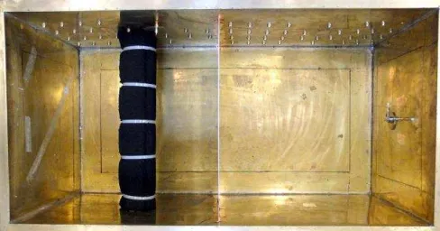
The predictions of the EDM were validated against measurements of the brass cavity shown in Fig. 10, which had the dimensions given in Table I. One wall of the cavity could be removed to allow access and another wall contained an array of holes into which a probe antenna could be inserted. The unused holes were closed by brass machine screws and nuts while the removable wall was clamped in place along a flange around the edge. Short monopole probe antennas where fabricated from SMA panel jacks.

An absorbing cylinder of radius 50 mm and height 450 mm was fabricated by rolling a sheet of radio absorbing material (RAM). For coupled cavity measurements an Aluminum partitioning plate of dimensions 450 mm × 410 mm was introduced at the midpoint of the cavity, leaving a 40 mm slot on the side of the cavity with the removable wall; this choice of geometry prevented contact issues between the partitioning plate and removable wall.

B. Measurement of diffuse fields

The mismatch corrected insertion gain,

between the two probes was determined from scattering parameters, , measured using a vector network analyzer at 1600 equi-spaced frequency points in the band 8-8.5 GHz. The diffuse field power density in the cavity was then estimated by averaging the insertion gain over the frequency band: c , i.e. by frequency stirring in the terminology of reverberation chamber measurement. The mode density in the cavity was about 10 MHz-1 _{at 8 GHz and the measured mode bandwidth was}

about 9 MHz when loaded, suggesting that about 50 independent samples of the field are included in the frequency average. Accordingly, the 1-sigma confidence interval on the measured average powers is about 1.3 dB [34].

C. Measurement of absorption factors

The total quality factor of the empty cavity at 8.5 GHz was estimated to be 25,000 from the average insertion gain. By fitting the effective conductivity of the walls using a PWB model of the cavity (including the antennas) to this Q-factor

the wall absorption efficiency was estimated to be .

The average absorption cross-section, , of the absorbing cylinder, with metal caps placed on either end, was measured in a reverberation chamber using the methodology described in [35]. At 8.5 GHz the measured absorption efficiency was found to be . This is somewhat higher than the prediction of (8) using the RAM

manufacturer’s complex permittivity ( ) to determine the Fresnel reflection coefficients, which gives . This is because the cylinder is in the resonant scattering regime at 8.5 GHz and the geometric optics approximation implicit in (8) is inaccurate.

D. Results

The average scalar power density was measured in the cavity, without the partition or absorbing cylinder, along a line with and with respect to the axes in Fig. 1. The measurements are shown in Fig. 11, compared to different model predictions. When the cavity is unloaded the measured power density is in very good agreement with PWB and the EDM; the two models give almost identical predictions so only the EDM result is shown in the figure for clarity.

For the cavity loaded with the absorbing cylinder (at the location of Example B in Table I) measurements were made with the monopole probes both co- and cross-polarized. The overall trend of the measurement results is in good agreement with the EDM solution using the Sabine absorption loss factor for the cylinder (7). Using the Jing & Xiang absorption factor (9) in the EDM gives a result that lies below the measurement data. The prediction of the PWB is also shown; it appears to underestimate the power density in the part of the cavity containing the source and overestimate it in the part containing the cylinder.

Placing the cylinder horizontally in the cavity of Fig. 10 it was also possible to measure the power density distribution in the plane of Fig. 1. The results are shown in Fig. 12 and are again consistent with the EDM, in particular the falling trend along the x-direction and the relative invariance in the y -direction. The statistical variation of the measurement data is

Fig. 10. Photograph, looking into the physical cavity (along the direction with respect to Fig. 1) used for the validation measurements. Monopole

probe antennas can be seen mounted on the “right” wall and the “roof” next

to the absorbing cylinder.

Author post-print 8

too large to allow a determination of the relative accuracy of the Sabine and Jing & Xiang absorption factor models, though there is some indication of a tendency towards the Jing & Xiang model with increasing distance from the source. The measurements above were repeated in the frequency band 16-16.5 GHz. With appropriate changes to the frequency dependent wall and cylinder absorption efficiencies in the EDM similar agreement was obtained.

Fig. 13 shows the results of measurements and models when the partition is introduced as in example B, but without the absorbing cylinder. The wall loss alone was sufficient to induce an approximately 2 dB difference in the diffuse field between the two cavities, which is predicted accurately by both the PWB model and EDM.

When the absorbing cylinder was introduced into the coupled cavity the results shown in Fig. 14 were obtained. The power level difference between the cavities is now about 10 dB. The general agreement is again good, though the measurements are somewhat more dispersed than the EDM prediction in the unloaded coupled cavity. The EDM does however predict the correct trend with variation in y. This deviation could be indicative of reduced diffusivity in the coupled cavity, beyond that which is predicted by (5)-(6). Further investigation of the effects of absorption and aperture

coupling on the local diffusivity is necessary.

VI. CONCLUSIONS

Diffusion equation based modeling of the diffuse electromagnetic field in enclosed spaces is a natural generalization of the PWB method already widely applied to EMC analysis. It is able to account for the inhomogeneous absorption that arises in many EMC applications, predicting the distribution of diffuse energy very efficiently compared to other techniques. For example, it can predict field non-uniformity in loaded reverberation chambers, informing the optimal positioning of antennas to minimize the systematic error due to the loading.

We have demonstrated the potential of the EDM technique using two canonical examples validated by measurement data, obtaining good results. The approach retains the flexibility of the traditional PWB model, allowing semi-empirical analysis of complex structures to be undertaken using experimentally determined absorption and transmission cross-section, but with greater accuracy due to the ability to deal with heterogeneous loss. It can also still be fully predictive if analytic expressions for all the required cross-sections are available.

A key advantage of the EDM technique is its computational efficiency; it can produce a solution in seconds using modest hardware for electrically large problems which can take many days to solve using full-wave techniques. This is very appealing for applications such as high frequency enclosure shielding assessment which can require onerous amounts of computing resource; a more efficiency approach could lead to significant cost savings in product development.

REFERENCES

[1] D. A. Hill, M. T. Ma, A. R. Ondrejka, B. F. Riddle, M. L. Crawford and

R. T. Johnk, “Aperture excitation of electrically large, lossy cavities”, IEEE Trans. Electromagn. Compat., vol. 36, no. 3, pp. 169-178, Aug. 1994.

[2] D. A. Hill, “Plane wave integral representation for fields in reverberation

chambers”, IEEE Trans. Electromagn. Compat., vol. 40, no. 3, pp. 209-217, Aug. 1998.

Fig. 12. Diffuse field scalar power density, normalized to 1 W source power, in the plane of the loaded cuboid cavity at 8.5 GHz, comparing measurement to PWB and diffusion models.

Fig. 13. Diffuse field scalar power density, normalized to 1 W source power, along four lines in the plane of the unloaded coupled cavities at 8.5 GHz, comparing measurement to PWB and diffusion models.

[3] I. Junqua, J.-P. Parmantier and F. Issac, “A network formulation of the power balance method for high-frequency coupling”, Electromagnetics, vol. 25, no. 7-8, pp. 603-622, 2005.

[4] J. B. Andersen, J. O. Nielsen, G. F. Pedersen, G. Bauch and M. Herdin,

“Room electromagnetics”, IEEE Antennas Propag. Mag., vol. 49, no. 2, pp. 27-33, April 2007.

[5] R. J. Pirkl and K. A. Remley, “Experimental evaluation of the statistical

isotropy of a reverberation chamber’s plane-wave spectrum”, IEEE Trans. Electromagn. Compat., vol. 56, no. 3, pp. 498-509, June 2014. [6] G. V. Gradoni, M. Primiani, and F. Moglie. “Dependence of

reverberation chamber performance on distributed losses: A numerical

study”, 2014 IEEE Int. Symp. Electromagn. Compat., Raleigh, NC, pp. 775-780, 4-8 Aug., 2014.

[7] I. D. Flintoft, G. C. R. Melia, M. P. Robinson, J. F. Dawson and A. C. Marvin, “Rapid and accurate broadband absorption cross-section

measurement of human bodies in a reverberation chamber”, IOPMeas. Sci. Techn., vol. 26, no. 6, art. No. 065701, pp. 1-9, Jun. 2015.

[8] K. A. Remley, J. Dortmans, C. Weldon, R. D. Horansky, T. B. Meurs, C.-M. Wang, D. F. Williams, C. L. Holloway P. F. Wilson,

“Configuring and verifying reverberation chambers for testing cellular

wireless devices”, IEEE Trans. Electromagn. Compat., vol. 58, no. 3, pp. 661-672, Jun. 2016.

[9] W. T. C. Burger, K. A. Remley, C. L. Holloway and J. M. Ladbury,

“Proximity and antenna orientation effects for large-form-factor devices

in a reverberation chamber”, 2013 IEEE Int. Symp.Electromagn. Compat., Denver, CO, pp. 671-676, 5-9 Aug., 2013.

[10] J. M. Navarro and J. Escolano, “Simulation of building indoor acoustics

using an acoustic diffusion equation model”, Journal of Building Performance Simulation, vol. 8, no. 1, pp. 3-14, 2015.

[11] L. Savioja and U. Peter Svensson, “Overview of geometrical room

acoustic modeling techniques”, J. Acoust. Soc. Am., vol. 138, no .2, pp. 708–730, 2015.

[12] J. M. Navarro, “Discrete time modeling of diffusion processes for acoustics simulation and analysis”, PhD thesis, Universidad Politécnica de Valencia, Departamento de Comunicaciones, Dec. 2011.

[13] J. Picaut, L. Simon and J.-D. Polack, “A mathematical model of diffuse

sound field based on a diffusion equation”, Acta Acustica, vol. 83, pp. 614–621, 1997.

[14] P. Morse and H. Feshbach, Methods of Theoretical Physics, McGraw-Hill, New York, 1953.

[15] V. Valeau, M. Hodgso, and J. Picaut, “A diffusion-based analogy for the

prediction of sound fields in fitted rooms”, Acta Acustica united with Acustica, vol. 93, no. 1, pp. 94–105, 2007.

[16] E. Amador, C. Lemoine, P. Besnier and A. Laisné, “Reverberation chamber modeling based on image theory: Investigation in the pulse

regime”, IEEE Transactions on Electromagnetic Compatibility, vol. 52, no. 4, pp. 778-789, Nov. 2010.

[17] W. C. Sabine, Collected Papers on Acoustics, Harvard University Press, 1922.

[18] D. A. Hill, “A reflection coefficient derivation for the Q of a

reverberation chamber”, IEEE Trans. Electromagn. Compat., vol. 38, no. 4, pp. 591-592, Nov. 1996.

[19] Y. Jing and N. Xiang, “Visualizations of sound energy across coupled

rooms using a diffusion equation model”, J. Acoust. Soc. Am., vol. 124, pp. EL360–EL365, Nov. 2008.

[20] A. Billon, J. Picaut and A. Sakout, “Prediction of the reverberation time

in high absorbent room using a modified diffusion model”, App. Acoust., vol. 69, no. 1, pp. 68–74, 2008.

[21] J. Escolano, J. M. Navarro and J. J. Lopez, “On the limitation of a diffusion equation model for acoustic predictions of rooms with homogeneous dimensions”, J. Acoust. Soc. Am., vol. 128, pp. 1586– 1589, 2010.

[22] G. Steinbock, T. Pedersen, B. H. Fleury, W. Wei and R. Raulefs,

“Experimental validation of the reverberation effect in room

electromagnetics”, IEEE Trans. Antennas Propag., vol. 63, no. 5, pp. 2041-2053, May 2015.

[23] V. Valeau, J. Picaut and M. Hodgson, “On the use of a diffusion equation for room-acoustic prediction”, J. Acoust. Soc. Am., vol. 119, no. 3, pp. 1504-1513, 2006.

[24] C. Visentin, N. Prodi and V. Valeau, “A numerical investigation of the

Fick’s law of diffusion in room acoustics”, J. Acoust. Soc. Am., vol. 132, no. 5, pp. 3180–3189, 2012.

[25] A. Billon, C. Foy, J. Picaut, V. Valeau and A. Sakout, “Modeling the sound transmission between rooms coupled through partition walls by

using a diffusion model”, J. Acoust. Soc. Am., vol. 123.6, pp. 4261– 4271, 2008.

[26] A. Gifuni, “Relation between the shielding effectiveness of an electrically large enclosure and the wall material under uniform and

isotropic field conditions”, IEEE Trans. Electromagn. Compat., vol. 55, no. 6, pp. 1354-1357, Dec. 2013.

[27] N. Xiang, J. Escolano, J. M. Navarro and Y. Jing, “Investigation on the

effect of aperture sizes and receiver positions in coupled rooms”, J. Acoust. Soc. Am., vol. 133, no. 6, pp. 3975–85, 2013.

[28] G. B. Tait, R. E. Richardson, M. B. Slocum and M. O. Hatfield, “Time -dependent model of RF energy propagation in coupled reverberant

cavities”, IEEE Trans. Electromagn. Compat., vol. 53, no. 3, pp. 846-849, Aug. 2011.

[29] L. V. Kantorovich and V. I. Krylov, Approximate Methods of Higher Analysis, 3rd edition, Interscience Publishers, New York, 1964. [30] M. E. Sequeira and V. H. Cortınez, “A simplified two-dimensional

acoustic diffusion model for predicting sound levels in enclosures”, App. Acoust., vol. 73, no. 8, pp. 842–848, 2012.

[31] F. Hecht, “New development in FreeFEM++”, Journal of Numerical Mathematics, vol. 20, no. 3-4, pp. 251–265, 2012.

[32] D. A. Hill, “Boundary fields in reverberation chambers”, IEEE Trans. Electromagn. Compat., vol. 47, no. 2, pp. 281-290, 2005.

[33] I. D. Flintoft, S. L. Parker, S. J. Bale, A. C. Marvin, J. F. Dawson and M.

P. Robinson, “Measured average absorption cross-sections of printed

circuit boards from 2 to 20 GHz”, IEEE Trans. Electromagn. Compat., vol. 58, no. 2, pp. 553-560, 2016.

[34] J. G. Kostas and B. Boverie, “Statistical model for a mode-stirred

chamber”, IEEE Trans. Electromagn. Compat., vol. 33, no. 4, pp. 366-370, Nov. 1991.

[35] X. Zhang, M. P. Robinson and I. D. Flintoft, “On measurement of reverberation chamber time constant and related curve fitting