This is a repository copy of
Synthesis of Probabilistic Models for Quality-of-Service
Software Engineering
.
White Rose Research Online URL for this paper:
http://eprints.whiterose.ac.uk/130619/
Version: Accepted Version
Article:
Gerasimou, Simos, Calinescu, Radu Constantin orcid.org/0000-0002-2678-9260 and
Tamburrelli, Giordano (2018) Synthesis of Probabilistic Models for Quality-of-Service
Software Engineering. Automated Software Engineering. ISSN 0928-8910
https://doi.org/10.1007/s10515-018-0235-8
[email protected] https://eprints.whiterose.ac.uk/
Reuse
Items deposited in White Rose Research Online are protected by copyright, with all rights reserved unless indicated otherwise. They may be downloaded and/or printed for private study, or other acts as permitted by national copyright laws. The publisher or other rights holders may allow further reproduction and re-use of the full text version. This is indicated by the licence information on the White Rose Research Online record for the item.
Takedown
If you consider content in White Rose Research Online to be in breach of UK law, please notify us by
(will be inserted by the editor)
Synthesis of Probabilistic Models for Quality-of-Service
Software Engineering
Simos Gerasimou · Radu Calinescu ·
Giordano Tamburrelli
Received: date / Accepted: date
Abstract An increasingly used method for the engineering of software sys-tems with strict quality-of-service (QoS) requirements involves the synthesis and verification of probabilistic models for many alternative architectures and instantiations of system parameters. Using manual trial-and-error or simple heuristics for this task often produces suboptimal models, while the exhaus-tive synthesis of all possible models is typically intractable. The EvoChecker search-based software engineering approach presented in our paper addresses these limitations by employing evolutionary algorithms to automate the model synthesis process and to significantly improve its outcome. EvoChecker can be used to synthesise the Pareto-optimal set of probabilistic models associated with the QoS requirements of a system under design, and to support the se-lection of a suitable system architecture and configuration. EvoChecker can also be used at runtime, to drive the efficient reconfiguration of a self-adaptive software system. We evaluate EvoChecker on several variants of three systems from different application domains, and show its effectiveness and applicability.
Keywords search-based software engineering·probabilistic model checking· evolutionary algorithms·QoS requirements
S. Gerasimou
Department of Computer Science, University of York Tel.: +44(0)1904325198
E-mail: [email protected]
R. Calinescu
Department of Computer Science, University of York Tel.: +44(0)1904325166
E-mail: [email protected]
G. Tamburelli lastminute.com
1 Introduction
Software systems used in application domains including healthcare, finance and manufacturing must comply with strict reliability, performance and other quality-of-service (QoS) requirements. The software engineers developing these systems must use rigorous techniques and processes at all stages of the software development life cycle. In this way, the engineers can continually assess the correctness of a system under development (SUD) and confirm its compliance with the required levels of reliability and performance.
Probabilistic model checking (PMC) is a formal verification technique that can assist in establishing the compliance of a SUD with QoS requirements through mathematical reasoning and rigorous analysis [12, 34]. PMC supports the analysis of reliability, timeliness, performance and other QoS requirements of systems exhibiting stochastic behaviour, e.g. due to unreliable components or uncertainties in the environment [69]. The technique has been successfully applied to the engineering of software for critical systems [6, 95]. In PMC, the behaviour of a SUD is defined formally as a finite state-transition model whose transitions are annotated with information about the likelihood or timing of events taking place. Examples of probabilistic models that PMC operates with include discrete and continuous-time Markov chains, and Markov decision pro-cesses [70]. QoS requirements are expressed formally using probabilistic vari-ants of temporal logic, e.g., probabilistic computation tree logic and continuous stochastic logic [70]. Through automated exhaustive analysis of the underly-ing low-level model, PMC proves or disproves compliance of the probabilistic model of the system with the formally specified QoS requirements.
Recent advances in PMC reinforced its applicability to the cost-effective engineering of software both at design time [11, 25, 72] and at runtime [26, 40]. The design-time use of the technique involves the verification of alternative de-signs of a SUD. The objectives are to identify dede-signs whose quality attributes comply with system QoS requirements and also to eliminate early in the design process errors that could be hugely expensive to fix later [37]. Designs that meet these objectives can then be used as a basis for the implementation of the system. Alternatively, software engineers can construct probabilistic mod-els of existing systems and employ PMC to assess their QoS attributes. Within the last decade, PMC has also been used to drive the reconfiguration of self-adaptive systems [14, 28, 42] by supporting the “analyse” and “plan” stages of the monitor-analyse-plan-execute control loop [24, 88] of these systems. In this runtime use, PMC provides formal guarantees that the reconfiguration plan adopted by the self-adaptive system meets the QoS requirements [20, 26]. We discuss related research on using PMC at runtime, including our recent work from [23, 50], in Section 8.
at-tributes of the system (e.g. the maximisation of reliability and minimisation of cost). Existing approaches such as exhaustive search and simple heuristics like manual trial-and-error and automated hill climbing can only tackle this challenge for small systems. Exhaustively searching the solution space for an optimal probabilistic model is intractable for most real-world systems. On the other hand, trial-and-error requires manual verification of numerous alterna-tive instantiations of the system parameters, while simple heuristics do not generalise well and are often biased towards a particular area of the problem landscape (e.g. through getting stuck at local optima).
The EvoChecker search-based software engineering approach presented in our paper addresses these limitations of existing approaches by automating the synthesis of probabilistic models and by considerably improving the outcome of the synthesis process. EvoChecker achieves these improvements by using evolutionary algorithms (EAs) to guide the search towards areas of the search space more likely to comprise probabilistic models that meet a predefined set of QoS requirements. These requirements can include bothconstraints, which specify bounds for QoS attributes of the system (e.g. “Workflow executions must complete successfully with probability at least 0.98”), andoptimisation objectives (e.g. “The workflow response time should be minimised”).
Given this set of QoS requirements and aprobabilistic model template that encodes the configuration parameters (e.g., alternative architectures, parame-ter ranges) of the software system, EvoChecker supports both the identification of suitable architectures and configurations for a software system under design, and the runtime reconfiguration of a self-adaptive software system.
When used at design time, EvoChecker employs multi-objective EAs to synthesise (i) a set of probabilistic models that closely approximates the Pareto-optimal model set associated with the QoS requirements of a software system; and (ii) the corresponding approximate Pareto front of QoS attribute values. Given this information, software designers can inspect the generated solutions to assess the tradeoffs between multiple QoS requirements and make informed decisions about the architecture and parameters of the SUD.
The main contributions of our paper are:
– The EvoChecker approach for the search-based synthesis of probabilistic models for QoS software engineering, and its application to the synthesis of models that meet QoS requirements both at design time and at runtime.
– The EvoChecker high-level modelling language, which extends the mod-elling language used by established probabilistic model checkers such as PRISM [71] and Storm [39].
– The definition of the probabilistic model synthesis problem.
– An incremental probabilistic model synthesis technique for the efficient run-time generation of probabilistic models that satisfy the QoS requirements of a self-adaptive system.
– An extensive evaluation of EvoChecker in three case studies drawn from different application domains.
– A prototype open-source EvoChecker tool and a repository of case studies, both of which are freely available from our project webpage at http://
www-users.cs.york.ac.uk/simos/EvoChecker.
These contributions significantly extend the preliminary results from our conference paper on search-based synthesis of probabilistic models [53] in sev-eral ways. First, we introduce an incremental probabilistic model synthesis technique that extends the applicability of EvoChecker to self-adaptive soft-ware systems. Second, we devise and evaluate different strategies for selecting the archived solutions used by successive EvoChecker synthesis tasks at run-time. Third, we extend the presentation of the EvoChecker approach with ad-ditional technical details and examples. Fourth, we use EvoChecker to develop two self-adaptive systems from different application domains (service-based systems and unmanned underwater vehicles). Finally, we use the systems and models from our experiments to assemble a repository of case studies available on our project website.
The rest of the paper is organised as follows. Section 2 presents the software system used as a running example. Section 3 introduces the EvoChecker mod-elling language, and Section 4 presents the specification of EvoChecker con-straints and optimisation objectives using the QoS requirements of a software system. Section 5 describes the use of EvoChecker to synthesise probabilistic models at design time and at runtime. Section 6 summarises the implementa-tion of the EvoChecker prototype tool. Secimplementa-tion 7 presents the empirical evalu-ation carried out to assess the effectiveness of EvoChecker, and an analysis of our findings. Finally, Sections 8 and 9 discuss related work and conclude the paper, respectively.
2 Running Example
Fig. 1: Workflow of the FX system (adapted from [53])
used by a European foreign exchange brokerage company and implements the workflow in Figure 1.
An FX trader can use the system to carry out trades in expert ornormal
mode. In the expert mode, the trader can provide her objectives or action strategy. FX periodically analyses exchange rates and other market activity, and automatically executes a trade once the trader’s objectives are satisfied. In particular, aMarket watch service retrieves real-time exchange rates of se-lected currency pairs. ATechnical analysisservice receives this data, identifies patterns of interest and predicts future variation in exchange rates. Based on this prediction and if the trader’s objectives are“satisfied”, an Order service is invoked to carry out a trade; if they are “unsatisfied”, execution control returns to the Market watch service; and if they are “unsatisfied with high variance”, an Alarm service is invoked to notify the trader about opportuni-ties not captured by the trading objectives. In thenormal mode, FX assesses the economic outlook of a country using aFundamental analysis service that collects, analyses and evaluates information such as news reports, economic data and political events, and provides an assessment of the country’s cur-rency. If the trader is satisfied with this assessment, she can sell/buy currency by invoking theOrder service, which in turn triggers aNotification service to confirm the successful completion of a trade.
The FX system usesmi≥1 functionally equivalent implementations of the i-th service. For any servicei, the j-th implementation, 1≤j≤mi is
charac-terised by its reliabilityrij∈[0,1] (i.e., probability of successful invocation),
invocation costcij∈R+ and response timetij∈R+.
Table 1: QoS requirements for the FX system
ID Informal description
R1“Workflow executions must complete successfully with probability at least 98%” R2“The total service response time per workflow execution should be minimised” R3“The probability of a service failure during a workflow execution should be minimised” R4“The total cost of the third-party services used by a workflow execution should be
minimised”
• ifstri = PROB, FX uses aprobabilistic strategy to randomly select one of
the service implementations based on an FX-specified discrete probability distribution pi1, pi2, . . . , pimi; and
• if stri = SEQ, FX uses a sequential strategy that employs an execution
order to invoke one after the other all enabled service implementations until a successful response is obtained or all invocations fail.
For the SEQ strategy, a parameter exi ∈ {1,2, ..., mi!} establishes which
of the mi! permutations of the mi implementations should be used, and a
configuration parameter xij ∈ {0,1}indicates if implementationj is enabled
(xij = 1) or not (xij = 0).
3 EvoChecker Modelling Language
EvoChecker uses an extension of the modelling language that leading model checkers such as PRISM [71] and Storm [39] use to define probabilistic models. This language is based on the Reactive Modules formalism [5], which models a system as the parallel composition of a set ofmodules. The state of amodule
is defined by a set of finite-range local variables, and its state transitions are specified by probabilistic guarded commands that modify these variables:
[action]guard−> e1:update1+. . .+en:updaten; (1)
where guard is a boolean expression over all model variables. If theguard is
true, the arithmetic expressionei,1≤i≤n, gives the probability (for
discrete-time models) or rate (for continuous-discrete-time models) with which the updatei
change of the module variables occur. Theactionis an optional element of type ‘string’; when used, all modules comprising commands with the same action
must synchronise by performing one of these commands simultaneously. For a complete description of the modelling language, we refer the reader to the PRISM manual atwww.prismmodelchecker.org/manual.
EvoChecker extends this language with the following three constructs that support the specification of the possible configurations of a system.
1. Evolvable parameters. EvoChecker uses the syntax
evolve intparam[min..max];
to define model parameters of type ‘int’ and ‘double’, respectively, and accept-able ranges for them. These parameters can be used in any field of command (1) other thanaction.
2. Evolvable probability distributions. The syntax
evolve distributiondist [min1..max1]. . .[minn..maxn]; (3)
where [mini,maxi] ⊆[0,1] for all 1≤ i ≤n, is used to define an n-element
discrete probability distribution, and ranges for thenprobabilities of the dis-tribution. The name of the distribution with 1,2, . . . , n appended as a suffix (i.e.,dist1,dist2, etc.) can then be used instead of expressionse1, e2, . . . , en
from ann-element command (1).
3. Evolvable modules. EvoChecker uses the syntax
evolve module modName implementation1endmodule . . .
evolve module modName implementationn endmodule
(4)
to definen≥2 alternative implementations of a modulemodName.
The interpretation of the three EvoChecker constructs within a probabilistic model template is described by the following definitions.
Definition 1 (Probabilistic model template)A valid probabilistic model augmented with EvoChecker evolvable parameters (2), probability distribu-tions (3) and modules (4) is called aprobabilistic model template.
Definition 2 (Valid probabilistic model) A probabilistic model M is an
instance of a probabilistic model templateT if and only if it can be obtained fromT using the following transformations:
– Each evolvable parameter (2) is replaced by a ‘const int param = val;’ or
‘const doubleparam = val;’ declaration (depending on the type of the
pa-rameter), whereval∈ {min, . . . , max} orval∈[min..max], respectively.
– Each evolvable probability distribution (3) is removed, and the n occur-rences of its name instead of expressions e1, . . . , en of a command (1)
are replaced with values from the ranges [min1..max1], . . . , [minn..maxn],
respectively. For a discrete-time model, the sum of the nvalues is 1.0.
– Each set of evolvable modules with the same name is replaced with a single element from the set, from which the keyword ‘evolve’ was removed.
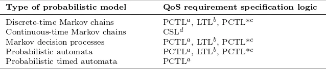
Table 2: Types of probabilistic models supported by EvoChecker
Type of probabilistic model QoS requirement specification logic
Discrete-time Markov chains PCTLa, LTLb, PCTL*c
Continuous-time Markov chains CSLd
Markov decision processes PCTLa, LTLb, PCTL*c
Probabilistic automata PCTLa, LTLb, PCTL*c
Probabilistic timed automata PCTLa
a
Probabilistic Computation Tree Logic [17, 56] b
Linear Temporal Logic [83]
c
PCTL* is a superset of PCTL and LTL d
Continuous Stochastic Logic [10, 13]
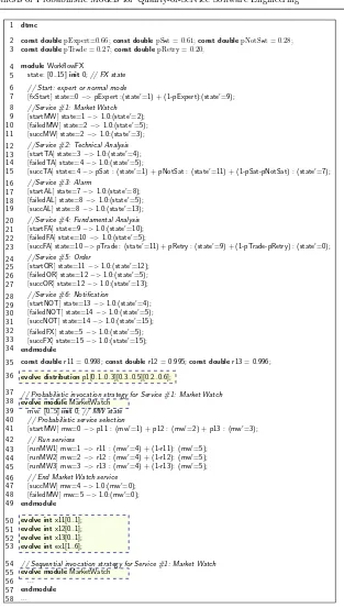
Example 1 Figure 2 presents the discrete-time Markov chain (DTMC) proba-bilistic model template of the FX system introduced in Section 2. The template comprises aWorkflowFXmodule modelling the FX workflow, and two modules modelling the alternative implementations of each service. These two service modules correspond to the probabilistic invocation strategy and the sequential invocation strategy, respectively. Due to space constrains, Figure 2 shows in full only theMarketWatchmodule for the probabilistic strategy of theMarket
watch service; the complete FX probabilistic model template is available on our project webpage.
The local variable state from theWorkflowFXmodule (line 5 in Figure 2) encodes the state of the system, i.e. the service being invoked, the success or failure of that service invocation, etc. The local variable mw from the Mar-ketWatch implementations (line 39) records the internal state of the Market watch service invocation. The WorkflowFXmodule synchronises with the ser-vice modules through ‘start’-, ‘failed’- and ‘succ’-prefixed actions, which are associated with the invocation, failed execution, and successful execution of a service, respectively. For instance, the synchronisation with the MarketWatch
module occurs through the actions startMW, failedMW and succMW (lines 9–11).
Each service module models a specific invocation strategy, e.g. a proba-bilistic selection is made between three available Market watch service im-plementations in line 41 of the first MarketWatchmodule. Then, the selected
service implementation is invoked (lines 43–45) and either completes success-fully (line 47) or fails (line 48). The FX system continues with the rest of its workflow (lines 12–31 from WorkflowFX) if the service executed successfully, or terminates (line 32) otherwise.
All three EvoChecker constructs (2)–(4) are used by the FX probabilistic model template:
– four evolvable parameters specify the enabled Market watch service im-plementations and their execution order (lines 50–53) associated with the sequential invocation strategy;
– an evolvable distribution specifies the discrete probability distribution for the probabilistic invocation strategy of the firstMarketWatchmodule (line 36);
1 2 3 4 5 6 7 8 9 10 11 12 13 14 15 16 17 18 19 20 21 22 23 24 25 26 27 28 29 30 31 32 33 34 35 36 37 38 39 40 41 42 43 44 45 46 47 48 49 50 51 52 53 54 55 56 57 58 dtmc
const doublepExpert=0.66;const doublepSat = 0.61;const doublepNotSat = 0.28;
const doublepTrade = 0.27;const doublepRetry = 0.20;
moduleWorkflowFX
state: [0..15]init0;// FX state
// Start: expert or normal mode
[fxStart]state=0−>pExpert :(state’=1) + (1-pExpert):(state’=9);
//Service #1: Market Watch
[startMW]state=1−>1.0:(state’=2);
[failedMW]state=2−>1.0:(state’=5);
[succMW]state=2−>1.0:(state’=3);
//Service #2: Technical Analysis
[startTA]state=3−>1.0:(state’=4);
[failedTA]state=4−>1.0:(state’=5);
[succTA]state=4−>pSat : (state’=1) + pNotSat : (state’=11) + (1-pSat-pNotSat) : (state’=7);
//Service #3: Alarm
[startAL]state=7−>1.0:(state’=8);
[failedAL]state=8−>1.0:(state’=5);
[succAL]state=8−>1.0:(state’=13);
//Service #4: Fundamental Analysis
[startFA]state=9−>1.0:(state’=10);
[failedFA]state=10−>1.0:(state’=5);
[succFA]state=10−>pTrade : (state’=11) + pRetry : (state’=9) + (1-pTrade-pRetry) : (state’=0);
//Service #5: Order
[startOR]state=11−>1.0:(state’=12);
[failedOR]state=12−>1.0:(state’=5);
[succOR]state=12−>1.0:(state’=13);
//Service #6: Notification
[startNOT]state=13−>1.0:(state’=4);
[failedNOT]state=14−>1.0:(state’=5);
[succNOT]state=14−>1.0:(state’=15);
[failedFX]state=5−>1.0:(state’=5);
[succFX]state=15−>1.0:(state’=15);
endmodule
const doubler11 = 0.998;const doubler12 = 0.995;const doubler13 = 0.996;
evolve distributionp1[0.1..0.3][0.3..0.5][0.2..0.6];
// Probabilistic invocation strategy for Service #1: Market Watch evolve moduleMarketWatch
mw: [0..5]init0;// MW state // Probabilistic service selection
[startMW]mw=0−>p11 : (mw’=1) + p12 : (mw’=2) + p13 : (mw’=3); // Run services
[runMW1]mw=1−>r11 : (mw’=4) + (1-r11): (mw’=5);
[runMW2]mw=2−>r12 : (mw’=4) + (1-r12): (mw’=5);
[runMW3]mw=3−>r13 : (mw’=4) + (1-r13): (mw’=5); // End Market Watch service
[succMW]mw=4−>1.0:(mw’=0);
[failedMW]mw=5−>1.0:(mw’=0);
endmodule
evolve intx11[0..1];
evolve intx12[0..1];
evolve intx13[0..1]; evolve intex1[1..6];
// Sequential invocation strategy for Service #1: Market Watch evolve moduleMarketWatch
...
endmodule
[image:10.595.86.399.72.625.2]...
Table 3: QoS attributes for the FX system
QoS attribute Informal description FormulaΦi
attr1 Workflow reliability P=?[Fstate= 15]
attr2 Workflow response time Rtime=?[F state= 15∨state= 5]
attr3 Workflow invocation cost RinvocationCost=? [F state= 15∨state= 5]
4 EvoChecker Specification of QoS Requirements
4.1 Quality-of-Service Attributes
Given the probabilistic model templateT of a system, QoS attributes such as the response time, throughput and reliability of the system can be expressed in the probabilistic temporal logics from Table 2, and can be evaluated by applying probabilistic model checking to relevant instances of T. Formally, given the probabilistic temporal logic formulaΦfor a QoS attributeattr and an instance M of T (i.e. a probabilistic model corresponding to a system configuration being examined), the value of the QoS attribute is
attr=PMC(M, Φ), (5)
where PMC is the probabilistic model checking “function” implemented by tools such as PRISM and Storm.
Example 2 The QoS requirements of the FX system from our running example (shown in Table 1) are based on three QoS attributes. RequirementsR1 and
R3 refer to the probability of successful completion (i.e. the reliability) of FX workflow executions. This QoS attribute corresponds to the probabilistic computation tree logic (PCTL) formulaP=?[F state= 15] from the first row of
Table 3. This PCTL formula expresses the probability that the probabilistic model template from Figure 2 reaches its success state.
The QoS attributes for the other two requirements can be specified using
rewards PCTL formulae [7, 64,69]. For this purpose, positive values are associ-ated with specific states and transitions of the model template from Figure 2 by adding the following tworewards. . . endrewardsstructures to the template:
rewards “time” rewards“invocationCost”
[runMW1]true :t11; [runMW1]true :c11;
[runMW2]true :t12; [runMW1]true :c12;
[runMW3]true :t13; [runMW1]true :c13;
. . . . . .
endrewards endrewards
These structures support the computation of the total service response time for requirement R2and of the workflow invocation cost for requirementR4. To this end, the two structures associate the mean response timetij and the
that models the execution of this service implementation. The corresponding PCTL formulae, shown in the last two rows of Table 3, represent the reward (i.e. the response time and cost, respectively) “accumulated” before reaching a state where the workflow execution terminates. In these formulae,state= 15 denotes a successful termination, andstate= 5 an unsuccessful one.
Before describing the formalisation of QoS requirements in EvoChecker, we note that a software system has two types of parameters:
1. Configuration parameters, which software engineers can modify to select between alternative system architectures and configurations. The EvoCheck-er constructs (2)–(4) are used to define these parametEvoCheck-ers and their accept-able values. The set of all possible combinations of configuration parameter values forms the configuration space Cfg of the system.
2. Environment parameters, which specify relevant characteristics of the envi-ronment in which the system will operate or is operating. These parameters cannot be modified, and need to be estimated based on domain knowledge or observations of the actual system. The set of all possible combinations of environment parameter values forms theenvironment space Env of the system.
A probabilistic model templateT of a system with configuration spaceCfgand environment spaceEnv corresponds to a specific combination of environment parameter valuese∈Env and to the entire configuration spaceCfg. Further-more, each instance M of T is associated with the same environment state
eand with a specific combination of configuration parameter values c∈Cfg. We will use the notation M(e, c) to refer to this specific instance of T, and the notationattr(e, c) for the value of a QoS attribute (5) computed for this instance.
Example 3 The environment parameters of the FX system comprise:
– the probabilitiespExpert,pSat,pNotSat,pTrade andpRetry from module
WorkflowFXin Figure 2;
– the success probabilities rij, response times tij and costs cij of the FX
service implementations.
The FX configuration parameters defined by the EvoChecker constructs from Figure 2 are:
– the invocation strategiesstri used for thei-th FX service;
– the probabilitiespij of invoking thej-th implementation of serviceiwhen
the probabilistic invocation strategy is used;
– the xij and exi parameters specifying which implementations of servicei
are used by the sequential invocation strategy and their execution order.
4.2 Quality-of-Service Requirements
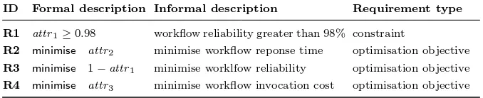
Table 4: Formal specification of QoS requirements for the FX system
ID Formal description Informal description Requirement type
R1 attr1≥0.98 workflow reliability greater than 98% constraint
R2 minimise attr2 minimise workflow reponse time optimisation objective R3 minimise 1−attr1 minimise worklfow reliability optimisation objective R4 minimise attr3 minimise workflow invocation cost optimisation objective
1. Constraints, i.e. requirements that specify bounds for the acceptable values of QoS attributes such as response time, throughput, reliability and cost. 2. Optimisation objectives, i.e. requirements which specify QoS attributes that
should be minimised or maximised.
Formally, EvoChecker considers systems withn1≥0 constraintsRC1, RC2, . . ., RC
n1, andn2≥1 optimisation objectivesR O
1, RO2, . . . , ROn2. Thei-th constraint,
RC
i , has the form
attri ⊲⊳iboundi (6)
and, assuming that all optimisation objectives require the minimisation of QoS attributes,1 thej-th optimisation objective,RO
j, has the form
minimiseattrn1+j, (7)
where ⊲⊳i∈ {<,≤,≥, >,=} is a relational operator,boundi ∈ R, 0 ≤ i≤n1,
1≤j≤n2, and attr1,attr2, . . . , attrn1+n2 representn1+n2 QoS attributes
(5) of the software system.
Example 4 The QoS requirements of the FX system (Table 1) comprise one constraint (R1) and three optimisation objectives (R2–R4). Table 4 shows the formalisation of these requirements for the design time use of EvoChecker using the FX QoS attributes from Table 3.
5 EvoChecker Probabilistic Model Synthesis
EvoChecker supports both the selection of a suitable architecture and configu-ration for a software system under design, and the runtime reconfiguconfigu-ration of a self-adaptive software system. There are three key differences between these two uses of EvoChecker.
First, the use of EvoChecker during system design requires the specification of the (fixed) environment state that the system will operate in by a domain expert, while for its runtime use the environment state is continually updated based on monitoring information.
Second, the EvoChecker use at design time can handle multiple optimisa-tion objectives and yields multiple Pareto-optimal soluoptimisa-tions (i.e. probabilistic
models). In contrast, EvoChecker at runtime yields a single solution (as synthe-sising multiple solutions is not useful without a software engineer to examine them) by operating with a single optimisation objective (i.e. a “loss” function). Finally, the use of EvoChecker for the design of a system is a one-off ac-tivity, whereas for a self-adaptive system the approach is used to select new system configurations on frequent intervals or after each environment change. The latter use involves the incremental synthesis of probabilistic models by generating each new configuration efficiently based on previously synthesised ones.
Given these differences between the design time and runtime EvoChecker uses, we present them separately in Sections 5.1 and 5.2, respectively.
5.1 Using EvoChecker at Design Time
5.1.1 Probabilistic Model Synthesis Problem
Consider a SUD with environment spaceEnv, an environment statee∈Env
provided by a domain expert, and a probabilistic model templateT associated with the configuration spaceCfg of the system. Given n1≥0 constraints (6)
andn2≥1 optimisation objectives (7), theprobabilistic model synthesis
prob-lem involves finding the Pareto-optimal set PS of configurations from Cfg
that satisfy then1 constraints and arenon-dominated with respect to then2
optimisation objectives:
PS ={c∈Cfg|∄c′∈Cfg•(∀0≤i≤n
1•attri(e, c)⊲⊳iboundi∧ attri(e, c′)⊲⊳iboundi)∧c′ ≺c}
(8)
with thedominance relation ≺:Cfg×Cfg→Bdefined by
∀c, c′∈Cfg•c≺c′≡ ∀n
1+ 1≤i≤n1+n2•attri(e, c)≤attri(e, c′)∧
∃n1+ 1≤i≤n1+n2•attri(e, c)<attri(e, c′).
Finally, given the Pareto-optimal setPS, thePareto front PF is defined by
PF ={(an1+1, an1+2, . . . , an1+n2)∈R n2 |
∃c∈PS • ∀n1+ 1≤i≤n1+n2•ai =attri(e, c)},
(9)
because the system designers need this information in order to choose between the configurations from the setP S.
5.1.2 Probabilistic Model Synthesis Approach
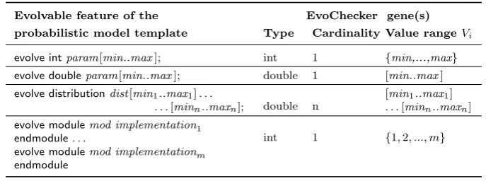
Table 5: EvoChecker gene encoding rules
Evolvable feature of the EvoChecker gene(s)
probabilistic model template Type Cardinality Value rangeVi
evolve intparam[min..max]; int 1 {min,...,max}
evolve doubleparam[min..max]; double 1 [min..max]
evolve distributiondist[min1..max1]. . .
. . .[minn..maxn]; double n
[min1..max1] . . . [minn..maxn] evolve modulemod implementation1
endmodule. . .
evolve modulemod implementationm endmodule
int 1 {1,2, ..., m}
evolvable parameters of type double) infinite. Therefore, EvoChecker synthe-sises a close approximation of the Pareto-optimal set by using standard multi-objective evolutionary algorithmssuch as the genetic algorithms NSGA-II [38], SPEA2 [100] and MOCell [81].
Evolutionary algorithms (EAs) encode each possible solution of a search problem as a sequence ofgenes, i.e. binary representations of the problem vari-ables. For EvoChecker, each use of an ‘evolvable’ construct (2)–(4) within the probabilistic model templateT contributes to this sequence with the gene(s) specified by the encoding rules in Table 5. EvoChecker uses these rules to ob-tain the value rangesV1, V2, . . . , Vk for thek≥1 genes of T, and to assemble
the SUD configuration spaceCfg =V1×V2× · · · ×Vk.
The high-level architecture of EvoChecker is shown in Figure 3. The prob-abilistic model template T of the SUD is processed by a Template parser
component. TheTemplate parser converts the template into an internal repre-sentation (i.e. a parametric probabilistic model) and extracts the configuration space Cfg as described above. The configuration spaceCfg and the n1 QoS
constraints andn2optimisation objectives of the SUD are used to initialise the
Multi-objective evolutionary algorithm component at the core of EvoChecker. This component creates a random initial population ofindividuals (i.e. a set of random gene sequences corresponding to differentCfg elements), and then iteratively evolves this population into populations containing “fitter” individ-uals by using the standard EA approach summarised next.
The EA approach involves evaluating different individuals (i.e., potential new system configurations) through invoking anIndividual analyser. This com-ponent combines an individual and the parametric model created by the Tem-plate parser to produce a probabilistic model M in which all configuration parameters are fixed using values from the genes of the analysed individ-ual. Next, the Individual analyser invokes a Quantitative verification engine
that uses probabilistic model checking to determine the QoS attributes attri,
1 ≤ i ≤ n1+n2, of the analysed individual. To this end, the Quantitative
Multi-objective evolutionary
algorithm
Individual analyser QoS constraints
and optimisation objectives
Formulae
Φ1, Φ2, ... , Φn1+n2 Probabilistic
model template T
Quantitative verification engine Template
parser
Pareto front approximation PF Config. space
Cfg= V1x V 2x ... x V k
Parametric model
Indi vidu
al
QoS att
ribu tes
QoS attribute attri
Model M, Formula Φi
Pareto-optimal set approximation PS
attr
1,..
.,att rn 1+
[image:16.595.71.410.81.202.2]n 2
Fig. 3: High-level EvoChecker architecture
attributes. These attributes are then used by theMulti-objective evolutionary algorithm to establish whether the individual satisfies then1 QoS constraints
and to assess its “fitness” based on the QoS attribute values associated with then2QoS optimisation objectives.
Once all individuals have been evaluated, theMulti-objective evolutionary algorithmperforms anassignment,reproductionandselectionstep. During as-signment, the algorithm establishes the fitness of each individual (e.g., its rank in the population). Fit individuals have higher probability to enter a “mating” pool and to be chosen for reproduction and selection. Withreproduction, the algorithm creates new individuals from the mating pool by means ofcrossover
and mutation. Crossover randomly selects two fit individuals and exchanges genes between them to produce offspring with potentially higher fitness val-ues. Mutation, on the other hand, introduces variation in the population by selecting an individual from the pool and creating an offspring by randomly changing a subset of its genes. Finally, throughselection, a subset of the indi-viduals from the current population and offspring becomes the new population that will evolve in the next generation.
TheMulti-objective evolutionary algorithmuseselitism, a strategy that di-rectly propagates into the next population a subset of the fittest individuals from the current population. This strategy ensures the iterative improvement of the Pareto-optimal approximation setP S assembled by EvoChecker. Fur-thermore, the multi-objective EAs used by EvoChecker maintain diversity in the population and generate a Pareto-optimal approximation set spread as uniformly as possible across the search space. This uniform spread is achieved using algorithm-specific mechanisms for diversity preservation. One such mech-anism involves combining thenondomination level of each evaluated individual and the population density in its area of the search space.2
Probabilistic model template T QoS constraints and optimisation
objective Software
system
Sensors Effectors
Monitor Formulae
Φ1, Φ2, ... , Φn1+1
EvoChecker
System configuration c
Environment state e
Archive of effective configurations with strategy σ System
configurations Ce
[image:17.595.73.408.73.175.2]Archived configurations
Fig. 4: EvoChecker-driven reconfiguration of self-adaptive software system
The evolution of fitter individuals continues until one of the following ter-mination criteria is met:
1. the allocated computation time is exhausted;
2. the maximum number of individual evaluations has been reached;
3. no improvement in the quality of the best individuals has been detected over a predetermined number of successive iterations.
Once the evolution terminates, the set of nondominated individuals from the final population is returned as the Pareto-optimal set approximationPS. The values of the QoS attributes associated with the n2 optimisation objectives
and with each individual from PS are used to assemble the Pareto front ap-proximationPF. System designers can analyse thePS andPF sets to select the design to use for system implementation.
5.2 Using EvoChecker at Runtime
5.2.1 EvoChecker-based Self-adaptive Systems
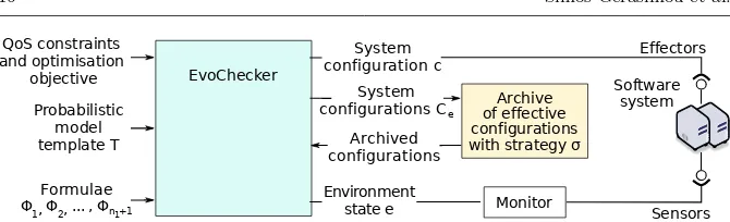
The use of EvoChecker to drive the runtime reconfiguration of self-adaptive software systems is illustrated in Figure 4. The approach uses systemSensors
to continually monitor the system and identify the parameters of the envi-ronment it operates in. Changes in the envienvi-ronment state e lead to updates of the probabilistic model templateT used by EvoChecker and to the incre-mental synthesis of a probabilistic model specifying a new configurationcthat enables the system to meet its QoS requirements in the changed environment. This configuration is applied using an Effectors interface of the self-adaptive system.
To speed up the search for a new configuration, the use of EvoChecker at runtime builds on the principles of incrementality and exploits the fact that changes in a self-adaptive system are typically localised [54]. As reported in other domains [61, 67], and also discussed in our related work section (Sec-tion 8), an effective initialisa(Sec-tion of the EA search can speed up its convergence and can yield better-quality solutions. Accordingly, EvoChecker maintains an
new search with a subset of recent configurations that encode solutions to potentially similar environment states experienced in the past.
To fully automate the EvoChecker operation, its runtime use combines the QoS requirements that target the optimisation of QoS attributes into a composite single objective. Similar to other approaches for developing self-adaptive systems [86], this objective requires the minimisation of a generalised
loss function given by
loss(e,c) =
n1+n2 X
j=n1+1
wj·attrj(e, c), (10)
wherewj ≥0 are weight coefficients and at least one of them is strictly
posi-tive.3
These weight coefficients express the desired trade-off between the j QoS at-tributes. Fonseca and Fleming [45] show that for any positive set of coefficient values, the identified solution is always Pareto optimal (compared to all other solutions generated during the search). Selecting appropriate values for the coefficients is a responsibility of system designers. To this end, they can use domain knowledge to determine the value range of the QoS attributes com-prising the loss function and assign appropriate coefficient values that reflect their relative importance [35]. Note that although more complex,lossis just another QoS attribute which can still be specified in the latest version of the probabilistic temporal logic languages supported by model checkers like PRISM [71], so it fits the definition of an attribute from equation (5).
Example 5 To use EvoChecker in a self-adaptive variant of the FX system from our running example, the QoS attributes from Table 3 need to be combined into aloss function (10) that the self-adaptive system should minimise, e.g.:
loss(e,c) =w1·(attr1(e, c))−1+w2·attr2(e, c) +w3·attr3(e, c),
with the weightsw1, w2 andw3chosen based on the value ranges and on the
relative importance of the three attributes. Note that the first attribute from the loss function is actually the reciprocal of the reliability attribute attr1
from Table 3, as we want decreases in reliability to lead to rapid increases in loss. Using the failure probability 1−attr1 as the first attribute is also an
option, although this choice yields alossfunction that increases only linearly with the failure probability.
5.2.2 Runtime Probabilistic Model Synthesis
When EvoChecker is used at runtime, the synthesis of probabilistic models is performed incrementally, i.e. by exploiting previously generated solutions, to
3
speed up the synthesis of new solutions. This incremental synthesis is enabled by theArchive component shown in Figure 4.
The use of EvoChecker within a self-adaptive system starts with an empty
Archive, which is updated at the end of each reconfiguration step using an
archive updating strategy. This strategy selects individuals from the final EA population synthesised by EvoChecker in the current reconfiguration step. Several criteria are used to enable this selection:
¬ an individual that meets all n1 constraints is preferred over an individual
that violates one or more constraints;
from two individuals that satisfy all constraints, the individual with the
lowestloss is preferred;
® from two individuals that both violate at least one constraint, the
individ-ual with the lowest overall “level of violation” is preferred.4
While EvoChecker is not prescriptive about the calculation of the level of vio-lation from the last criterion, the current version of our tool uses the following definition.
Definition 3 (Constraints violation)For each combination of an environ-ment statee∈Env and a configurationc∈Cfg of a self-adaptive system, the level of violation of then1QoS constraints is given by
violation(e, c) = X
1≤i≤n1 ¬(attri⊲⊳iboundi)
αi· |boundsi−attri(e, c)|, (11)
whereαi>0 is aviolation weight associated thei-th attribute.
Note that according to this definition, violation(e, c) = 0 for all (e, c) combi-nations that violate none of then1bounds.
Example 6 Consider the QoS requirements of the FX system from Table 1. The only QoS constraint, R1, requires that workflow executions are at least
bound1= 0.98 reliable. Hence, for any (e, c)∈Env×Cfg,
violation(e, c) =
α1· |0.98−attr1(e, c)|, ifattr1(e, c)<0.98
0, otherwise
The value of α1 (i.e., α1 = 100 in our experiments from Section 7.2) is
pro-vided to EvoChecker by simply annotating the constraintR1with this value. EvoChecker automatically parses all such annotations and constructs the vio-lation function for the system.
EvoChecker employs a preference relation based on criteria¬-®to select
configurations for storing in its archive. This relation and the EvoChecker
archive updating strategy are formally defined below.
4
Definition 4 (Preference relation) Let e∈Env be an environment state of a self-adaptive system, and violation : Env ×Cfg → R+ a function that
specifies the level of violation of then1 QoS constraints for each combination
(e, c)∈Env×Cfg.5 Then, given two configurationsc, c′ ∈Cfg, configuration
cispreferred over configurationc′ (writtenc≺c′) iff
∀1≤i≤n1•attri(e, c)⊲⊳i boundsi ∧
∃1≤i≤n1• ¬(attri(e, c′)⊲⊳iboundsi)∨ ¬
∀1≤i≤n1•attri(e, c)⊲⊳i boundsi ∧ attri(e, c′)⊲⊳iboundsi
∧loss(e, c)< loss(e, c′)
∨
∃1≤i, j≤n1• ¬(attri(e, c)⊲⊳iboundsi)∧ ¬(attrj(e, c′)⊲⊳jboundsj)
∧violation(e, c)<violation(e, c′) ®
Definition 5 (Archive updating strategy) Let Ce ⊆ Cfg be the set of
configurations synthesised for the new environment statee∈Env andArchbe the archive before the change. Then anarchive updating strategy is a function
σ:Cfg →Bsuch that the updated archive at the end of the reconfiguration step is given by
Arch′={c∈Arch∪Ce|σ(c)} (12)
We formally define four archive updating strategies that we will use to evaluate EvoChecker in Section 7:
1. Theprohibitive strategy retains no configurations in the archive:
σ(c) =false,∀c∈Arch∪Ce (13)
2. The complete recent strategy uses the entire population from the current adaptation step and removes the previous configurations from the archive:
σ(c) =
(
true, ifc∈Ce
false, otherwise (14)
3. Thelimited recent strategy keeps thex,0< x <#Ce, best configurations
from the current adaptation step and removes the previous configurations from the archive:
σ(c) =
(
true, ifc∈Ceandposition(c)≤x
false, otherwise , (15)
whereposition:Ce→ {1,2, . . . ,#Ce}is a function that gives the position
of a configurationc∈Ce, i.e.position(c) = #{c′∈Ce\ {c} |c′≺c}+ 1.
5
For instance, for any (e, c) the violation function may count the number of violated QoS constraints, i.e.,violation(e, c) = #{1 ≤i≤n1 | ¬(attri(e, c)⊲⊳iboundsi)}, or may
4. Thelimited deep strategy accumulates thex,0≤x≤#Cebest
configura-tions from all previous adaptation steps, given by
σ(c) =
true, ifc∈Ceandposition(c)≤x true, ifc∈Arch
false, otherwise
(16)
As the limited deep strategy yields archives that grow in size after each reconfiguration step, some of the archive elements must be evicted when the archive size exceeds the size of the EA population. Possible eviction meth-ods include: (i) discarding the “oldest” individuals (e.g. by implementing the archive as a circular buffer of size equal to that of the EA population); and (ii) performing a random selection.
Using the archiveArchto create the initial EA population is carried out by importing configurations from the archive into the population (cf. Figure 4). If a complete population cannot be created in this way (e.g. because Arch is empty at the beginning of the first reconfiguration step and may not contain sufficient individuals for a few more steps), additional individuals are generated randomly to form a complete initial population.
Theassignment,reproduction andselection operations applied during the iterative evolution of the population, and the EA termination criteria are sim-ilar to those from the design-time use of EvoChecker. However, a standard
single-objective (generational) evolutionary algorithm is used instead of the multi-objective evolutionary algorithm, since there is only one optimisation objective (10).
6 Implementation
To ease the evaluation and adoption of the EvoChecker approach, we have im-plemented a tool that automates its use at both design time and runtime. Our EvoChecker tool uses the leading probabilistic model checker PRISM [71] as its
Quantitative verification engine, and the established Java-based framework for multi-objective optimization with metaheuristics jMetal [41] for its (Multi-objective) Evolutionary algorithm component. We developed the remaining EvoChecker components in Java, using the Antlr6 parser generator to build
the Template parser, and implementing dedicated versions of the Individual analyser,Monitor,Sensor andEffector components.
The open-source code of EvoChecker, the full experimental results sum-marised in the following section, additional information about EvoChecker and the case studies used for its evaluation are available at http://www-users.
cs.york.ac.uk/simos/EvoChecker.
7 Evaluation
We performed a wide range of experiments to evaluate the effectiveness of EvoChecker at both design time and runtime. The design-time use of Evo-Checker employs multi-objective genetic algorithms (MOGAs), while the run-time use of EvoChecker is based on a single-objective (generational) Genetic algorithm (GA). Experimenting with other types of evolutionary algorithms (e.g. evolution strategies, differential evolution) is part of our future work (Section 9). In Sections 7.1 and 7.2, we describe the evaluation procedure and the results obtained for the design-time and runtime use of EvoChecker, re-spectively. For each use, we introduce the research questions that guided the experimental process, we describe the experimental setup, we summarise the methodology followed for obtaining and analysing the results, and finally, we present and discuss our findings. We conclude the evaluation with a review of threats to validity (Section 7.3).
7.1 Evaluating EvoChecker at Design Time
7.1.1 Research Questions
The aim of our evaluation was to answer the following research questions.
RQ1 (Validation): How does the design-time use of EvoChecker per-form compared to random search?
We used this research question to establish if the application of EvoChecker at design time “comfortably outperforms a random search” [59], as ex-pected of effective search-based software engineering solutions.
RQ2 (Comparison): How do EvoChecker instances using different MOGAs perform compared to each other?
Since we devised EvoChecker to work with any MOGA, we examined the results produced by EvoChecker instances using three established such al-gorithms (i.e., NSGA-II [38], SPEA2 [100], MOCell [81]).
RQ3 (Insights): Can EvoChecker provide insights into the tradeoffs between the QoS attributes of alternative software architectures and instantiations of system parameters?
To support system experts in their decision making, EvoChecker must provide insights into the tradeoffs between multiple QoS objectives. To address this question, we identified a range of decisions suggested by the EvoChecker results for the software systems considered in our evaluation.
7.1.2 Experimental Setup
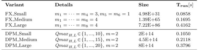
Table 6: Analysed system variants for EvoChecker at design time
Variant Details Size Trun[s]
FX Small m1=· · ·=m4= 3, m5=m6= 1 4.98E+31 0.0858
FX Medium m1=· · ·=m6= 4 1.39E+65 0.1695
FX Large m1=· · ·=m8= 4 7.22E+86 0.4162
DPM Small QmaxH,L∈ {1, ...,10},m= 2 2E+14 0.1050
DPM Medium QmaxH,L∈ {1, ...,15},m= 2 4.5E+14 0.2118
DPM Large QmaxH,L∈ {1, ...,20},m= 2 8E+14 0.3796
a software-controlled dynamic power management (DPM) system adapted from [85, 90] and described on our project webpage.
We performed a wide range of experiments using the system variants from Table 6. The column ‘Details’ reports the number of third-party implementa-tions for each service of the FX system7; and the capacity of the two request
queues (QmaxH and QmaxL) and the number of power managers available
(m= 2) for the DPM system. The column ‘Size’ lists the configuration space size assuming a two-decimal points discretisation of the real parameters and probability distributions of the probabilistic model template (cf. Table 5). Given the nonlinearity of most probabilistic models, this is the minimum pre-cision we could assume as an 0.01 increase or decrease in one of these parame-ters can have a significant effect in the evaluation of a QoS attribute. Finally, the column ‘Trun’ shows the average running time per system variant for
eval-uating a configuration. Note that the EvoChecker run time depends on the size of modelMand the time consumed by the probabilistic model checker to establish then1+n2 QoS attributes from equation (5) and on the computer
used for the evaluation.
We conducted a two-part evaluation for EvoChecker. First, to assess the stochasticity of the approach when different MOGAs are adopted and also to eliminate the possibility that any observations may have been obtained by chance, we used specific scenarios for the system variants from Table 6. For the FX system variants, we chose realistic values for reliability, performance and invocation cost of third-party services implementations, while the values of parameters for the DPM system variants (i.e., power usage and transition rates) correspond to the real-world system from [85, 90]. Second, to mitigate further the risk of accidentally choosing values that biased the EvoChecker evaluation, we defined a set of 30 different scenarios per FX system variant with varied services characteristics for each scenario.
7.1.3 Evaluation Methodology
We used the following established MOGAs to evaluate the use of EvoChecker at design time: NSGA-II [38], SPEA2 [100] and MOCell [81].
7
In line with the standard practice for evaluating the performance of stochas-tic optimisation algorithms [9], we performed multiple (i.e., 30) independent runs for each system variant from Table 6 and each multiobjective optimisa-tion algorithm, i.e., NSGA-II, SPEA2, MOCell and random search. Each run comprised 10,000 evaluations, each using a different initial population of 100 individuals, single-point crossover with probability pc = 0.9, and single-point
mutation with probabilitypm= 1/np, wherenpis the number of configuration
parameters for a particular system variant. All the experiments were run on a CentOS Linux 6.5 64bit server with two 2.6GHz Intel Xeon E5-2670 processors and 32GB of memory.
Obtaining the actual Pareto front for our system variants is unfeasible because of their very large configuration spaces. Therefore, we adopted the es-tablished practice [99] of comparing the Pareto front approximations produced by each algorithm with the reference Pareto front comprising the nondomi-nated solutions from all the runs carried out for the analysed system variant. For this comparison, we employed the widely-used Pareto-front quality indi-cators below, and we will present their means and box plots as measures of central tendency and distribution, respectively:
Iǫ (Unary additive epsilon) [102]. This is the minimum additive term by
which the elements of the objective vectors from a Pareto front approxima-tion must be adjusted in order to dominate the objective vectors from the reference front. This indicator presents convergence to the reference front and is Pareto compliant8. Smaller I
ǫ values denote better Pareto front
approximations.
IHV (Hypervolume) [101]. This indicator measures the volume in the
ob-jective space covered by a Pareto front approximation with respect to the reference front (or a reference point). It measures both convergence and diversity, and is strictly Pareto compliant [98]. Larger IHV values denote
better Pareto front approximations.
IIGD (Inverted Generational Distance) [93]. This indicator gives an
“er-ror measure” as the Euclidean distance in the objective space between the reference front and the Pareto front approximation. IIGD shows both
di-versity and convergence to the reference front. SmallerIIGD values signify
better Pareto front approximations.
We used inferential statistical tests to compare these quality indicators across the four algorithms [9, 60]. As is typical of multiobjective optimisa-tion [99], the Shapiro-Wilk test showed that the quality indicators were not normally distributed, so we used the Kruskal-Wallis non-parametric test with 95% confidence level (α= 0.05) to analyse the results without making assump-tions about the distribution of the data or the homogeneity of its variance. We also performed a post-hoc analysis with pairwise comparisons between the al-gorithms using Dunn’s pairwise test, controlling the family-wise error rate with the Bonferroni correctionpcrit=α/k, where kis the number of comparisons.
8
Table 7: Mean quality indicator values for a specific scenario of the FX system variants (top) and DPM system variants (bottom) from Table 6.
Variant NSGA-II SPEA2 MOCell Random
Iǫ(Epsilon)
FX Small 0.6258 0.5083 0.6745 2.2274 +
FX Medium 1.6379 2.0105 2.0486 6.1529 +
FX Large 3.8528 5.2777 4.6366 13.0234 +
IHV (Hypervolume)
FX Small 0.611 0.628 0.608 0.593 +
FX Medium 0.719 0.725 0.702 0.606 +
FX Large 0.657 0.675 0.633 0.555 +
IIGD (Inverted Generational Distance)
FX Small 0.00123 0.00129 0.00125 0.00145 +
FX Medium 0.00192 0.00207 0.00200 0.00316 +
FX Large 0.00244 0.00255 0.00272 0.00395 +
Variant NSGA-II SPEA2 MOCell Random
Iǫ(Epsilon)
DPM Small 0.0209 0.0130 0.0242 0.1403 +
DPM Medium 0.0225 0.0123 0.0489 0.1996 +
DPM Large 0.0229 0.0147 0.0884 0.2497 +
IHV (Hypervolume)
DPM Small 0.4455 0.4458 0.4396 0.4022 +
DPM Medium 0.4487 0.4499 0.4386 0.3946 +
DPM Large 0.4528 0.4549 0.4395 0.3947 +
IIGD (Inverted Generational Distance)
DPM Small 0.00023 0.00018 0.00016 0.00062 +
DPM Medium 0.00024 0.00019 0.00028 0.00091 +
DPM Large 0.00024 0.00020 0.00038 0.00109 +
7.1.4 Results and Discussion
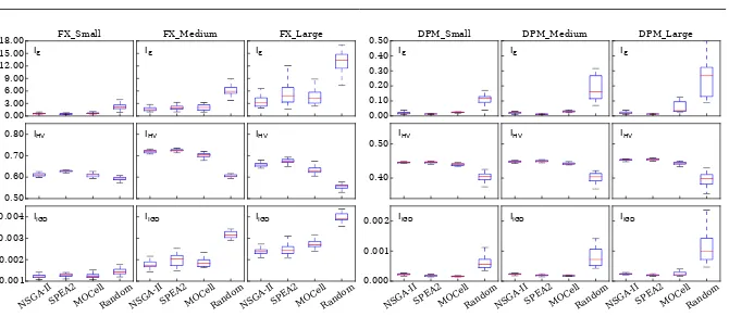
RQ1 (Validation). We carried out the experiments described in the pre-vious section and we report their results in Table 7 and Figure 5. The ‘+’ from the last column of the table entries indicate that the Kruskal-Wallis test showed significant difference among the four algorithms (p-value<0.05) for all six system variants and all Pareto-front quality indicators.
0.00 3.00 6.00 9.00 12.00 15.00 18.00 0.50 0.60 0.70 0.80 NSG A-II SPEA 2 MOC ell Rand om 0.001 0.002 0.003 0.004 NSG A-II SPEA 2 MOC ell Rand om NSG A-II SPEA 2 MOC ell Rand om
FX_Small FX_Medium FX_Large
Iε Iε Iε
IHV IHV IHV
IIGD IIGD IIGD
0.00 0.10 0.20 0.30 0.40 0.50 0.40 0.50 NSG A-II SPEA 2 MOC ell Rand om 0.000 0.001 0.002 NSG A-II SPEA 2 MOC ell Rand om NSG A-II SPEA 2 MOC ell Rand om
DPM_Small DPM_Medium DPM_Large
Iε Iε Iε
IHV IHV IHV
[image:26.595.75.410.76.222.2]IIGD IIGD IIGD
Fig. 5: Boxplots for a specific scenario of the FX system variants (left) and DPM system variants (right) from Table 6, evaluated with quality indicators
Iǫ,IHV andIIGD.
We qualitatively support our findings by showing in Figures 6 and 7 the Pareto front approximations achieved by EvoChecker with each of the MOGAs and by random search, for a typical run of the experiment for the DPM and FX system variants, respectively. We observe that irrespective of the MOGA, EvoChecker achieves Pareto front approximations with more, better spread and higher quality nondominated solutions than random search.
As explained earlier, the parameters we used for the DPM system variants (power usage, transition rates, etc.) correspond to the real-world system [85, 90]. In contrast, for the FX system variants we chose realistic values for the reliability, performance and cost of the third-party services. To mitigate the risk of accidentally choosing values that biased the EvoChecker evaluation, we performed additional experiments comprising 300 independent runs per FX system variant (900 runs in total) in which these parameters were randomly instantiated. To allow for a fair comparison across the experiments comprising the 30 different FX scenarios, and to avoid undesired scaling effects, we nor-malise the results obtained for each quality indicator per experiment within the range [0,1]. The results of this further analysis, shown in Table 8 and Figure 8, validate our findings.
Considering all these results, we have strong empirical evidence that the EvoChecker significantly outperforms random search, for a range of system variants from two different domains, and across multiple widely-used MOGAs. This also confirms the challenging and well-formulated nature of the multi-objective probabilistic model synthesis problem we introduced in Section 5.1.1.
RQ2 (Comparison). To compare EvoChecker instances based on differ-ent MOGAs, we first observe in Table 7 that NSGA-II and SPEA2 out-performed MOCell for all system variant–quality indicator combinations ex-cept DPM Small (IIGD). Between SPEA2 and NSGA-II, the former achieved
0.96 0.92 1.00 30 45 60 75 90 16 18 20 22 Relia bility Cost T im e [ s
] NSGA-IISPEA2
MOCell Random
(a) FX Small
Relia bility 0.96 0.92 1.00 20 40 60 80 100 16 20 24 28 Cost T im e [ s ] NSGA-II SPEA2 MOCell Random
(b) FX Medium
0.96 0.92 1.00 60 90 120 150 30 35 40 25 45 Relia bility Cost T im e [ s ] NSGA-II SPEA2 MOCell Random
[image:27.595.71.409.71.174.2](c) FX Large
Fig. 6: Typical Pareto front approximations for the FX system variants and optimisation objectives R2–R4 from Table 4.
0.801.20 1.602.00 0.00 0.03 0.06 0.09 0.12 0.0 2.5 5.0 7.5 Q u e ue l e ng th
qH +
q
L
SPEA2 Random
Los t reque
sts Power us e [W]
(a) DPM Small
0.00 0.03 0.06 0.09 0.12 Los t reque
sts 0.80
1.201.60 2.00
Power us
e [W]
0 3 6 9 12 NSGA-II Random Q u e ue l e ng th qH + q L
(b) DPM Medium
0.801.20
1.602.00
Power us e [W]
0.00 0.03 0.06 0.09 0.12 Los t re quests 0 4 8 12 Q u e ue l e ng th qH + q L NSGA-II SPEA2 MOCell Random
(c) DPM Large
Fig. 7: Typical Pareto front approximations for the DPM system variants. The DPM optimisation objectives involve minimising the steady-state power utili-sation (“Power use”), minimising the number of requests lost at the steady state (“Lost requests”), and minimising the capacity of the DPM queues (“Queue length”).
variants), whereas NSGA-II yielded Pareto-front approximations with better
Iǫ and IIGD indicators for the larger configuration spaces of the FX system
variants (except the combination FX Small (Iǫ)).
Additionally, we carried out the post-hoc analysis described in Section 7.1.3, for 9 system variants (counting separately the FX system variants with chosen services characteristics and those comprising the adaptation scenarios) × 3 quality indicators = 27 tests. Out of these tests, 22 tests (i.e., a percentage of 81.4%) showed high statistical significance in the differences between the per-formance achieved by EvoChecker with different MOGAs (Table 9). The five system variant–quality indicator combinations for which the tests were unsuc-cessful are: FX Medium (Iǫ), FX Small Adapt (Iǫ), FX Medium Adapt(Iǫ),
FX Small(IIGD) and FX Medium(IIGD).
[image:27.595.65.412.221.309.2]Table 8: Mean quality indicator values across 30 different scenarios for the FX system variants from Table 6
Variant NSGA-II SPEA2 MOCell Random
Iǫ(Epsilon)
FX Small 0.2212 0.2209 0.2272 0.6200 +
FX Medium 0.3393 0.3664 0.3645 0.7568 +
FX Large 0.3396 0.3764 0.3625 0.7970 +
IHV (Hypervolume)
FX Small 0.9374 0.9914 0.9337 0.9016 +
FX Medium 0.9514 0.9848 0.9219 0.8138 +
FX Large 0.9467 0.9804 0.8962 0.7868 +
IIGD (Inverted Generational Distance)
FX Small 0.6365 0.5348 0.6390 0.8000 +
FX Medium 0.5919 0.5790 0.6114 0.7957 +
FX Large 0.5887 0.5622 0.6561 0.8884 +
0.00 0.20 0.40 0.60 0.80 1.00
Iǫ
0.70 0.80 0.90 1.00
IHV
NSGA-IISPEA2MOCellRandom 0.20
0.40 0.60 0.80 1.00
IIGD
NSGA-IISPEA2MOCellRandomNSGA-IISPEA2MOCellRandom
FX_Small FX_Medium FX_Large
Fig. 8: Boxplots for the FX system variants (Table 6) across 30 different sce-narios, evaluated using the quality indicatorsIǫ,IHV andIIGD.
RQ3 (Insights). We performed qualitative analysis of the Pareto front ap-proximations produced by EvoChecker, in order to identify actionable insights. We present this for the FX and DPM Pareto front approximations from Fig-ures 6 and 7, respectively.
Table 9: System variants for which the MOGAs in rows are significantly better than the MOGAs in columns
NSGA-II SPEA2 MOCell
1 2 3 4 5 6 7 8 9 1 2 3 4 5 6 7 8 9 1 2 3 4 5 6 7 8 9
N
S
G
A
-I
I
Iǫ 3 3 3 3
IHV 3 3 3 3 3 3 3
IIGD 3 3
S
P
E
A
2 I
ǫ 3 3 3 3 3 3 3
IHV 3 3 3 3 3 3 3 3 3 3 3 3 3 3 3
IIGD3 3 3 3 3 3 3 3 3
MO
C
e
ll
Iǫ IHV
IIGD3 3 3
Key: 1:DPM Small, 2:DPM Medium, 3:DPM Large, 4:FX Small, 5:FX Medium, 6:FX Large, 7:FX Small Random, 8:FX Medium Random, 9:FX Large Random
request loss. This key information helps system experts to avoid unnecessarily expensive solutions.
Second, we note the high density of solutions in the areas with low relia-bility (below 0.95) for the FX system in Figure 6, and with high request loss (above 0.09) for the DPM system in Figure 7. For the FX system, for instance, these areas correspond to the use of the probabilistic invocation strategy, for which numerous service combinations can achieve similar reliability and re-sponse time with relatively low, comparable costs. Opting for a configuration from this area will make the FX system susceptible to failures, as when the only implementation invoked for an FX service fails, the entire workflow execution will also fail. In contrast, reliability values above 0.995 correspond to expensive configurations that use the sequential selection strategy; e.g., FX Small must use the sequential strategy for the Market watch and Fundamental analysis
services in order to achieve 0.996 reliability.
Third, the EvoChecker results reveal configuration parameters that QoS attributes are particularly sensitive to. For the FX system, for example, we no-ticed a strong dependency of the workflow reliability on the service invocation strategy and the number of implementations used for each service. Configura-tions from high-reliability areas of the Pareto front not only use the sequential strategy, but also require multiple services per FX service (e.g., three FX ser-vice providers are needed for success rates above 0.99).
7.2 Evaluating EvoChecker at Runtime
7.2.1 Research Questions
We evaluated the runtime use of EvoChecker to answer the research questions below.
RQ4 (Effectiveness): Can EvoChecker support dependable adapta-tion?With this research question we examine whether our approach can identify new effective configurations at runtime.
RQ5 (Validation): How does EvoChecker perform compared to ran-dom search? Following the standard practice in search-based software engineering [60], with this research question we aim to determine whether our approach performs better than random search.
RQ6 (Archive-strategy comparison): How do EvoChecker instances based on different archive updating strategies compare to each other? We used this research question to analyse the impact of various
archive updating strategies in the performance of EvoChecker. To this end, we study whether specificstrategiesimprove the quality of a search and/or help identifying faster an effective configuration. We also investigate possi-ble relationships between archive updating strategies and specific adapta-tion events.
7.2.2 Experimental Setup
For the experimental evaluation, we used two self-adaptive software systems from different application domains. The first is the FX service-based system from Section 2 and the second is an embedded system from the area of un-manned underwater vehicles (UUVs) adapted from [23, 50, 51] and described on our project webpage.
We applied EvoChecker at runtime to the system variants from Table 10, aiming to assess its behaviour for multiple configuration space sizes. As before (cf. Table 6), the column ‘Details’ shows for the UUV system the number of sensors, their measurement rates and the UUV speed, while for the FX system the number of third-party implementations for each service. The column ‘Size’ reports the size of the configuration space that an exhaustive search would need to explore using two-decimal precision for the real parameters and probability distributions of the probabilistic model template (cf. Table 5). Finally, the column ‘Trun’ shows the average time required by EvoChecker to evaluate a
configuration on a 2.6GhZ Intel Core i5 Macbook Pro computer with 16GB memory, running Mac OSX 10.9.
Table 10: Analysed system variants for the runtime EvoChecker
Variant Details Size Trun[s]
UUV Medium m= 5, r1, r2, . . . , r5∈[0Hz,8Hz],sp∈[0,10m/s] 1.04E+19 0.0076 UUV Large m= 10, r1, r2, . . . , r10∈[0Hz,8Hz],sp∈[0,10m/s] 1.09E+35 0.1622
FX Small m1=· · ·=m4= 3, m5=m6= 1 4.98E+31 0.0312
FX Medium m1=· · ·=m6= 4 1.39E+65 0.0953
Table 11: QoS requirements for the UUV system
ID Informal description
R1“The UUV must take at least 500 accurate measurements for each 100m travelled” R2“The UUV sensors must not consume more than 1000 Joules per 100m travelled” R3“The speed with which the UUV travels should be maximised”
R4“The energy consumed by the UUV sensors should be minimised”
of QoS requirements) and therefore are forced to adapt. Sensors in the UUV variants, beyond normal behaviour, encounter periods of unexpected changes (C1-C12) during which their rates change dramatically, including sensor fail-ures and recovery from these failfail-ures, and significant variation in measurement rates. Changes C1–C13 in FX comprise sudden minor or significant increase in response time and decline in reliability of service implementations, and com-plete failure or recovery of service implementations. For instance, change C7 in FX Small represents a deviation from the nominal reliability of the first and third service implementations of theMarket Watch service (cf. Figure 2): be-fore the change,r11= 0.98 andr13= 0.993; and, after the change,r11= 0.89
and r13 = 0.93. This is a significant change because the FX system cannot
meet the reliability requirement (Table 1) using only the degraded service im-plementations (i.e., x11= 1, x12= 0, x13= 1). Instead, a valid configuration
should always realise the functionality of the Market Watch service by se-lecting its second service implementation (thus setting x12 = 1).9 We make
available the EvoChecker templates for the changes in Table 12 on our project webpage.
Answering research question RQ1entails making the configuration space size tractable for exhaustive search. Searching exhaustively through the con-figuration space of the UUV Medium variant (which has the smallest config-uration space and the shortest average time per evaluation) would take an estimated 2.19·1013hours (given the 1.04·1019configurations to analyse, and
a mean analysis time of 0.0076 seconds). Thus, we used the UUV Medium variant but disabled three of its sensors, leaving just under 2.56·109 possible
configurations. We also disregarded the adaptation time, since it is too large for exhaustive search. For the same reason, we performed this assessment on
9
![Fig. 1: Workflow of the FX system (adapted from [53])](https://thumb-us.123doks.com/thumbv2/123dok_us/1968923.157947/6.595.112.402.81.245/fig-workow-fx-adapted.webp)