This is a repository copy of
An adaptive finite element procedure for fully-coupled point
contact elastohydrodynamic lubrication problems
.
White Rose Research Online URL for this paper:
http://eprints.whiterose.ac.uk/81231/
Article:
Ahmed, S, Goodyer, CE and Jimack, PK (2014) An adaptive finite element procedure for
fully-coupled point contact elastohydrodynamic lubrication problems. Computer Methods in
Applied Mechanics and Engineering, 282. 1 - 21. ISSN 0045-7825
https://doi.org/10.1016/j.cma.2014.08.026
[email protected] https://eprints.whiterose.ac.uk/ Reuse
Unless indicated otherwise, fulltext items are protected by copyright with all rights reserved. The copyright exception in section 29 of the Copyright, Designs and Patents Act 1988 allows the making of a single copy solely for the purpose of non-commercial research or private study within the limits of fair dealing. The publisher or other rights-holder may allow further reproduction and re-use of this version - refer to the White Rose Research Online record for this item. Where records identify the publisher as the copyright holder, users can verify any specific terms of use on the publisher’s website.
Takedown
If you consider content in White Rose Research Online to be in breach of UK law, please notify us by
An adaptive finite element procedure for fully-coupled point contact
elastohydrodynamic lubrication problems
Sarfraz Ahmed
∗1, Christopher E. Goodyer
2, and Peter K. Jimack
31Department of Mathematics, Hazara University, Mansehra, Pakistan
2,3School of Computing, University of Leeds, UK
Abstract
This paper presents an automatic locally adaptive finite element solver for the
fully-coupled EHL point contact problems. The proposed algorithm uses a posteriori error
estimation in the stress in order to control adaptivity in both the elasticity and the
lubrication domains. The implementation is based on the fact that the solution of the linear elasticity equation exhibits large variations close to the the fluid domain
on which the Reynolds equation is solved. Thus the local refinement in such region
not only improves the accuracy of the elastic deformation solution significantly but
also yield an improved accuracy in the pressure profile due to increase in the spatial resolution of fluid domain. Thus, the improved traction boundary conditions leads to
even better approximation of the elastic deformation. Hence, a simple and an
effec-tive way to develop an adapeffec-tive procedure for the fully-coupled EHL problem is to
apply the local refinement to the linear elasticity mesh. The proposed algorithm also seeks to improve the quality of refined meshes to ensure the best overall accuracy. It
is shown that the adaptive procedure effectively refines the elements in the region(s)
showing the largest local error in their solution, and reduces the overall error with
op-timal computational cost for a variety of EHL cases. Specifically, the computational cost of proposed adaptive algorithm is shown to be linear with respect to problem
size as the number of refinement levels grows.
KEYWORDS: elastohydrodynamic lubrication; finite element method; linear elasticity; fully
coupled approach; adaptive h-refinement; optimization of meshes
1 INTRODUCTION
The use of lubricants between the moving components of mechanical systems helps protect them
from direct contact, and therefore reduces both friction and wear. This in turn leads to less energy
consumption and increased life of the machine components respectively. To keep the moving components apart in the presence of a thin lubricant film, a pressure is generated in the film due
to the relative motion of the components. Generally, for non-conforming contacts, the pressure
generated is very high, which causes a significant elastic deformation in the contact surfaces and hence defines a new shape of the lubricant film. Such a class of problem is known as
elastohy-drodynamic lubrication (EHL) [1, 2, 13, 18, 42, 43].
The shape of the lubricant film depends upon the geometry of the contacts and the
resul-tant elastic deformation of the contacting surfaces. A most commonly used method to calculate
the elastic deformation of the surfaces is based upon evaluation of an elastic deformation inte-gral [13,19,29,42,43] which is obtained by an analytical solution of the linear elasticity equation
on a semi-infinite domain. A number of efficient numerical techniques have been developed over
the past few decades using this half-space approach, for example the multilevel multi-integration (MLMI) method [9]. Historically, the most common approaches for discretizing the lubrication
equation have been based on finite difference schemes [17, 42]. These methods limit the
dis-cretization process to regular structured rectangular meshes using low order approximations, and have been combined effectively with the use of multigrid method [29]. Typically, these difference
schemes are loosely coupled with the elastic deformation equation, which allows the efficient
combination of multigrid and MLMI [42, 43], but with a slowly converging outer iteration for heavily-loaded cases.
An alternative solution technique is the fully-coupled approach, which consists of solving the
discretized elasticity and lubrication equations simultaneously, see for example [25, 33, 34], with the goal of obtaining a faster convergence rate for the iterative solution. These examples are based
on the half-space approach for the elastic deflection. The drawback of this approach is that it uses
the pressure from all points in the domain to calculate the deflection at each point, which makes the resulting linearized system matrix dense. Furthermore, for heavy loads, the Jacobian matrix
becomes almost singular, which makes it hard to reach the solution. A “differential deflection
method” was introduced by Evans and Hughes [15, 23, 24, 26]. The advantage of this method is that it uses information from comparatively fewer points in the domain to calculate the elastic
deflection at each point. In other words the influence of pressure acting at a point is reduced to a limited locality of that point. Therefore this approach results in a less dense matrix compared to
the traditional half-space approach for elastic deflection.
Habchi et al. [20–22] also used a fully-coupled approach to solve the EHL problems. This technique is different however since it replaced the half-space solution method with the direct
finite element approximation of the linear elasticity equation on a finite contact domain. The
resultant system of discrete equations is therefore very large but is sparse. The author used a sparse direct solver to solve the linearized system at each Newton iteration. Sparse direct solvers
are very efficient for small systems but as the resolution and/or the dimension of the problem
highly sparse fully-coupled systems. This solution method leads to substantial savings in mem-ory and time. Most importantly, both the memmem-ory and the time growth, with respect to problem
size, is shown to be linear. For circular point contact cases, the authors used manually-generated
3D meshes for the linear elasticity approximation, which were based on a large number of exper-iments in order to obtain a satisfactory EHL solution at the lowest cost as possible. Note that, in
the selection of those meshes, smaller mesh spacings were used only in the contact region where the pressure solution exhibits the largest variation [17, 28]. Similarly, the solution of the linear
elasticity equation also exhibits large variations close to the contact region. Hence, the mesh
el-ements closest to the contact region are shown to have the largest errors both in the pressure and the linear elasticity solutions [1].
In this paper, the development of an automatic locally adaptive finite element solution scheme
for the fully-coupled EHL point contact problems is discussed, which refines the mesh in the contact as well as the elasticity domain based upon local error estimates for the stress. This
proposed algorithm therefore combines the several efficiency techniques [2, 38, 48, 49] to obtain
performance results that are comparable to those of multigrid and MLMI [42, 43], but with the side effect of predicting the interior deformation and stresses for the contacting elements. It will
be shown that the proposed procedure effectively refines the elements in the region(s) showing
the largest error in their solution, and reduces the overall error with optimal computational cost. Specifically, the growth in the computational cost of the whole adaptive solution process is shown
to be linear with respect to problem size as the number of adaptive levels grows.
2 MATHEMATICAL MODEL AND FULLY-COUPLED APPROACH
2.1 Mathematical model
In this subsection an isothermal EHL point contact model is presented in non-dimensional form.
The EHL point contact model considers an equivalent geometry of a contact where contact be-tween two surfaces is represented by an elastic surface and a rigid plane. Note that the equivalent
elastic surface contains the total elastic properties of the original contact surfaces, and hence the
solution will define the total elastic deformation of both contacting surfaces [2, 21].
2.1.1 Reynolds equation: This governs the pressure distribution through the contact region
(Ωf) for the given geometry and properties of lubricant. It reads (e.g. [1, 43]):
∇.(ǫ∇P)− ∂
∂X (¯ρH) = 0, (1)
whereǫ= ρH¯ηλ¯ 3, P andHare the (unknown) dimensionless pressure and film thickness
Dowson and Higginson [13] density model are used, although the conclusions are not dependent upon these specific choices.
Finally, it is generally assumed that the pressure is equal to the ambient pressure at the
bound-ary of the contact region. Pressure lower than the vapour pressure is physically unacceptable, thus the fluid will cavitate and the pressure will remain equal to the vapour pressure. This
pro-cess is called cavitation [14, 16, 42]. Since atmospheric and vapour pressure are generally very small compared to the pressure generated inside the contact region they are treated as zero in this
model. Hence the pressure throughout the contact is bounded below by zero. Thus, together with
the principle of mass conservation [14], the Reynolds boundary conditions reads:
P = 0 on ∂Ωf and ∇P.~n= 0 at the cavitation boundary,
where~nis the outward normal vector to the cavitation boundary and ∂Ωf is the boundary of
computational region. Note that this is a free boundary problem since the location of cavitation boundary is not known prior to computing the pressure solution. Amongst the various possible
treatments to handle this free boundary problem (see for example [14, 16, 44]), this work
consid-ers a penalty method introduced by Wu [44]. This introduces an additional term (known as the penalty term) for which the modified Reynolds equation reads:
∇.(ǫ∇P)− ∂
∂X (¯ρH)−ξP
−= 0, throughoutΩ
f, (2)
whereP = 0on∂Ωf,ξis a suitably large positive number andP−= min(P,0). This term has
an affect of forcing any negative pressure towards zero, and only dominates in the regions where
P <0.
2.1.2 Film thickness equation: This determines the shape of the lubricant film in the contact.
For the circular point contact case (with non-dimensional radius of curvature equal to one)
H=H0+X
2+Y2
2 +D(X, Y), (3)
whereH0 is a central offset film thickness andD is the elastic deformation [1, 21] (see
Sec-tion 2.2).
2.1.3 Load balance equation: This is a conservation law which ensures that the total pressure
generated balances the applied load. For the non-dimensional point contact case this requires [1, 43]:
Z
Ωf
P(X, Y)dΩf =
2π
2.2 Linear elasticity equation:
In the film thickness equation, the elastic deformationDof the contacting bodies can be modelled
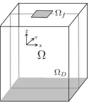
by solving Lam´e’s equation of linear elasticity on a three dimensional domainΩfor point contact problems (e.g. [1, 31], with appropriate boundary conditions):
∂
∂Xj
µ
Cijkl
∂Uk
∂Xl
= 0, (5)
where repeated suffices imply summation over the number of space dimensions (three),
Cijkl=λδijδkl+µ(δikδjl+δilδjk)
andλandµ(known as Lam´e’s coefficients) are material properties given by
λ= νE
(1 +ν)(1−2ν), µ=
E 2(1 +ν).
Hereδij is the Kronecker delta, whilstE is the equivalent Young’s modulus andν is the
equiv-alent Poisson ratio of the material used, see [22]. Note that the equation (5) is solved subject to
the boundary conditions:
U = 0 at the bottom boundaryΩD;
σn=njCijkl∂U∂Xkl =−δi3P at the fluid boundaryΩf;
σn= 0 elsewhere.
(6)
A view of the 3D domainΩ(showing the contact region as a fluid boundary (Ωf) and the bottom
boundary (ΩD)) is given in the Figure 1. In [21] it is demonstrated that a geometry of size
60×60×60is sufficiently large to provide accurate solutions for this non-dimensional model. Hence this elasticity domain is adopted throughout this paper (though a modification of this
domain would be of no significance to what follows). Note that D(X, Y) in equation (3) is
related to the displacement fieldUthrough the following relation:
D=−Uz |Ωf .
2.3 Fully-coupled approach
The solution of the EHL point contact problem consists of solving the Reynolds equation (2), the linear elasticity equation (5) and the load balance equation (4). These EHL equations may
be discretized using the Galerkin finite element method. However, since the Reynolds equation
exhibits an oscillatory behaviour in the pressure solution for heavily-loaded cases (see [29, 43] for example), in order to get a stabilized solution a Streamline Upwind Petrov Galerkin (SUPG)
Figure 1: A view of the 3D elasticity domainΩshowingΩf (the fluid boundary) andΩD (the
bottom boundary)
The fully-coupled approach involves the direct coupling of all of the discrete systems
aris-ing from the finite element discretization of the EHL equations to form a nonlinear system of
algebraic equations for all unknowns (i.e. the3elastic displacements at each point in the finite element mesh coveringΩ, the pressure approximation at each point in the mesh coveringΩf and
the value ofH0). This monolithic system is solved in one pass using a Newton solver. Typically,
such a solver converges for all loadings provided a sufficiently good initial guess is used (see Section 5 for a more detailed discussion of this).
The discrete nonlinear system may be expressed in the following vector form:
RP(P,U, H0) =0 RU(P,U) =0
RH0(P) = 0 .
(7)
Here RP represents the system of np nonlinear equations arising from the discretization of
Reynolds equation, RU is the linear system of 3×nu equations arising from discretization
of the linear elasticity equation andRH0 is the scalar residual of the discretized load balance
equation. Similarly,Pis a vector of thenp unknown pressure coefficients,Uis a vector of the
3×nuunknown displacement components andH0is the unknown central offset.
When a Newton’s method is applied to system (7), the following linear system is obtained at each outer iteration:
∂RP
∂P
∂RP
∂U
∂RP
∂H0
∂RU
∂P
∂RU
∂U 0
∂RH
0
∂P 0
T 0 δP δU δH0 =
−RP −RU −RH0
Starting with an initial estimate for the solution, the Newton procedure consists of solving the linearized system (8) at each Newton iteration and this update is added to the solution obtained
at the previous iteration, to provide an improved solution. This process is repeated until
con-vergence is achieved. The details of the solution of the linearized systems (8) are discussed in next section. If the initial guess is not sufficiently accurate then some under-relaxation may be
required to achieve the convergence.
3 SOLUTION PROCEDURE
In this section we discuss the overall layout of the new adaptive algorithm used in this work. A
suitable initial mesh is first generated using NETGEN [37], where a finer mesh is used in the
contact region compared to the other parts of the domain. The selection of a graded initial mesh permits a better starting solution than for a uniform coarse grid however the specific choice for
this mesh will be shown to be non-critical for the adaptive procedure. The high-level algorithm
used in this work can be split into the following steps.
0. Using the new mesh, build the corresponding data structures for the EHL solver.
1. Set up and solve the fully-coupled EHL problem using the solver described in [2].
2. Estimate the error within each element of the elasticity domainΩ. If the maximum
refine-ment level has been reached or all elerefine-ments have a sufficiently small error then output is produced and the code exits, otherwise a list of elements is created for refinement.
3. Perform h-refinement. If the mesh optimization option is selected then goto step 4, other-wise goto step 1.
4. Optimize the locally refined mesh. Free up all the previous data structures except for the new mesh and the solution data, and goto step 0.
In the following subsections, a detailed description is provided for each of the above steps involved in the adaptive procedure.
3.1 Solver
The adaptive procedure requires the solution of a nonlinear system (7) following each mesh re-finement/generation. As described in the previous section, a Newton procedure is applied to such
nonlinear systems, yielding a linear system (8) at each outer iteration. The solution of the
sys-tem (8) is the most expensive part of each Newton iteration. In this work, a right-preconditioned GMRES method [36] is used to solve (8) at each Newton iteration. The key feature (described
This is based upon approximating the∂RU
∂U block in (8) by a single algebraic or geometric multi-grid V-cycle [8, 10, 39] and using a fast sparse direct solver [12] for the (much smaller) ∂RP
∂P block of the preconditioner. Results presented in [2] show that this approach substantially
out-performs the application of a sparse direct solver to the whole of (8), both in terms of memory and of CPU requirements.
3.2 Error Estimation
Once the fully-coupled system is solved then the error within each element is estimated, using
an ‘a posteriori’ error estimation. An ‘a posteriori’ error assessment is based on the computed
numerical solution and is therefore an essential ingredient for any adaptive finite element proce-dure. Many such estimators have been developed, e.g. [4, 7] and references therein, however this
work is based upon the recovery approach first proposed by Zienkiewicz and Zhu [47–49].
3.2.1 An ‘a posteriori’ error estimate: By way of introduction, let us assume thatuhis a finite
element approximation to an exact solutionuof the linear elasticity equation. Then the error in
the computed solution is the difference:
e=u−uh,
and the error in their corresponding gradients or stresses, denoted byσ, is:
eσ =σ−σh.
For an elasticity problem, stresses are calculated from the finite element solution by:
σh =DSuh,
where the elasticity matrixDand the differential operatorSare given by [5] (for the3D
prob-lem):
D= E
(1+ν)(1−2ν)
1−ν ν ν 0 0 0
ν 1−ν ν 0 0 0
ν ν 1−ν 0 0 0
0 0 0 1−2ν
2 0 0
0 0 0 0 1−2ν
2 0
0 0 0 0 0 1−2ν
2
, S=
∂
∂x 0 0
0 ∂y∂ 0
0 0 ∂
∂z ∂ ∂y ∂ ∂x 0 0 ∂ ∂z ∂ ∂y ∂ ∂z 0 ∂ ∂x .
It is now possible to define the corresponding energy norm of the error for this problem, based
on the stresses of the solution, via the following expression [47]:
keσk2= Z
Ω
Since neither the exact solutionu nor σ are known, a reliable estimator of this error can be obtained if the true gradientsσare replaced with a suitable (higher order) approximationσ∗:
ke∗ σk2=
Z
Ω
(σ∗−σ
h)TD−1(σ∗−σh)dΩ. (9)
Generally the gradients computed from the finite element approximation are discontinuous over
the inter-element boundaries. A recovered approximation can be made at each node by averaging the elemental contribution of such gradients over the patch of elements sharing that node. It is
then possible to use the linear interpolating polynomials (the same as those used in the finite
el-ement approximation) to define a continuous, recovered, approximation over the whole domain. This class of methods are often known as averaging methods [4]. Various estimators can be
dis-tinguished based on the specific steps involved in the construction of the average or recovered gradients.
A well-known recovery-based error estimator was proposed by Zienkiewicz and Zhu [47]
(known variously as the Zienkiewicz-Zhu or ZZ or Z2 error estimator). Later on, these authors presented an improved estimator based on superconvergent patch recovery [48, 49]. These
esti-mators are based on the fact that there are points within the elements where the gradients are
more accurate and converge to exact values more quickly as the element size decreases. Specifi-cally, such points exhibit superconvergent behaviour in the solution and are therefore referred to
as superconvergent points. Thus a more accurate estimate(σ∗)of the true gradient(σ)is
recov-ered at a node by interpolating between the gradients at the superconvergent points in a patch of elements surrounding that node. Nevertheless, the standard ZZ error estimator is both
economi-cal and easy to implement, and it has been shown to be just as effective as many residual-based
error estimators in different comparative studies, see for example [5–7].
It should be noted that the norm used in (9) is defined over the whole domainΩ. In practice, the
squared value of the norm can be obtained by summing up the individual element contributions,
i.e.
ke∗ σk2 =
N
X
i=1 ke∗
σk2i, (10)
whereiis the element number,k.k2i is defined as in (9) but withΩreplaced the region occupied by elementi(Ωisay) andN is the total number of elements in the current mesh.
Recall that a fully-coupled EHL problem consists of solving the Reynolds equation, the linear
elasticity equation and the load balance equation simultaneously. For point contact problems, the linear elasticity equation is numerically solved on a3D domainΩ, while the Reynolds equation
is solved on a2D fluid domainΩf which is a small part of the boundary ofΩ. The solution of
the linear elasticity equation exhibits large variations close to the fluid region. This tends to lead to the mesh elements close to the fluid region having larger estimated errors. Performing local
refinement on these elements therefore improves the accuracy of the elastic deformation solution
inΩf leads to local refinement of the fluid domain on which the Reynolds equation is solved.
Together, the increase in the spatial resolution inΩf and the greater accuracy in the computed
elastic deformation yield a significantly improved accuracy in the pressure profile. This, in turn,
improves the traction boundary condition, to allow an even better approximation of the elastic deformation. Hence, our hypothesis is that a simple and effective way to develop an adaptive
procedure for the fully-coupled EHL problem is to apply local refinement to the linear elasticity mesh based upon local error estimation for the elastic stress alone. This hypothesis is explored
in sections 4 and 5 below, where its validity is demonstrated.
3.2.2 Refinement strategy: If the global error is already within the prescribed bounds for a
given mesh then the goal is already achieved. However, when this is not the case local refinement is necessary in those parts of the domain which exhibit the largest errors. In this work, a tolerance
(ηtol) is specified for the target relative error (η) in the computed stresses, i.e. :
η∗= ke∗σk
kσhk
≤ηtol. (11)
The refinement, solution and error estimation steps are repeated until this criterion is satisfied.
Unfortunately, it is not always possible to reach the target value (say ηtol = 0.05 [46]) for
the error (especially for the 3D problems) due to the availability of computer resources (e.g.
memory and CPU cycles). Therefore additional stopping criteria must also be specified, such
as maximum refinement levels, minimum element size, memory usage, etc. . In this work, the maximum number of refinement levels are used as a secondary stopping criterion for the adaptive
procedure.
As stated earlier, refinement is necessary in the regions of largest error. In other words, one feature of an optimal mesh is that the error is equally distributed among all the elements in the
mesh. Mathematically, this may be expressed as [32]:
ke∗
σki ≤ηtol
µ
kσhk2+ke∗σk2
N
1 2
=etol,
whereiis the element number,Nis the total number of elements andetol(average element error)
represents the maximum permissible error for an element. In other words, the ratio:
ξi =
ke∗ σki
etol
>1 (12)
specifies the set of elements to be refined. Derefinement is also possible, to save computations,
wheneverξi< ξderef ≪1: however this is not considered in this work.
all of the elements (emax) and targeting elements for refinement according to the equation:
etol=cemax. (13)
This is the approached used here, wherecis a selected constant (if not explicitly stated otherwise, a value of0.2is used in this work for demonstration purposes, however a comparison of different
values is provided in [1]). Note that any decrease in this parameter may result in flagging quite
a lot more elements for refinement and the required goal, of a near-optimal mesh, may not be achieved due to an excessive number of elements being refined at each stage.
3.3 Refinement
Once tetrahedral elements have been marked for refinement this is then implemented using the
TETRAD software [38]. The algorithm used in TETRAD is hierarchical in nature and is suitable for both mesh refinement and derefinement processes.
Only the mesh refinement routines are used here, based upon all edges of all of the marked
elements being tagged for refinement into two. If an edge is marked for refinement then it leads to refinement of all elements sharing that edge. The refinement process takes into account only
two types of subdivision. A regular subdivision in which each parent element is divided into eight
child elements by introducing new nodes bisecting each edge. In the first instance this leads to removal of four corners leaving an octahedron behind. The division of this octahedron further
results into four new child elements on the basis of dissection by the longest diagonal [27, 38].
The other kind of subdivision, the so-called green refinement, takes place where not all of the edges of an element are marked for refinement, and this avoids the possibility of introducing
“hanging nodes” (nodes on edges which are not the vertices of all elements sharing those edges)
without introducing any additional edge refinement. Note that green refinement often leads to poor quality elements, and therefore a precaution is taken into account in the development of
TETRAD that a green element may not be refined further. In such a case, the previous green
refinement of the parent element is replaced with regular refinement. Thus the green refinement always appears at the interface between lower and higher grid levels. As a consequence, the poor
quality elements never appear in the region of interest provided appropriate flagging criteria have been used for adaption. Finally, it should be noted that the scaling of the fundamental refinement
process is close to optimal linear behaviour [38] and is not significantly affected by the mesh
depth.
3.4 Optimization of Meshes
In [1], it is observed that the unstructured meshes resulting from hierarchical mesh refinement often lead to poor quality EHL results without appropriate mesh optimization. In other words,
local refinement process.
In order to combine optimization with local mesh refinement, the meshes obtained once the
refinement is performed are passed to NETGEN [37], where a smoothing process is performed
via edge and face swaps, local node movement, and some collapsing of elements. Note that, unlike [30], the optimization does not seek to reduce the error further, rather it is undertaken
to ensure minimization of a quality functional which quantifies the quality of the mesh. An advantageous side-effect of the optimization is that the collapsing of elements in the optimization
process also leads to a small reduction in the size of problem compared to the original mesh. A
difficulty encountered with this approach is how to handle transfer of the solution data between the grids before and after smoothing. Furthermore, the optimization processes destroys the mesh
hierarchy, so that neither de-refinement nor the use of geometric multigrid preconditioning is
easily possible.
Smoothing via NETGEN [37] also has the feature that the mesh optimization only takes place
in the interior of the domain, i.e. the surface mesh remains unchanged. The advantage of this
is that the latest estimate of the pressure solution can be transferred to the new optimized mesh without any difficulty. However, to produce an initial guess for the elasticity solution on this
changed mesh, one needs to solve the elasticity equation corresponding to the surface pressure.
Hence, at the cost of a solution of the elasticity equation (equivalent to less than the cost of one coupled Newton iteration) one obtains a consistent initial guess from which the
fully-coupled iteration converges very quickly. Note however that the next refinement of green2D
elements on the fixed surface mesh will lead to even more poor quality surface mesh elements, regardless of an optimized3D mesh. The poor quality surface mesh in the fluid region may affect
the accuracy of the pressure solution. One possibility to avoid the low quality surface mesh is
to perform the mesh optimization only at the final level of the mesh hierarchy, to improve the accuracy of the final solution. This is therefore considered as one of the possible strategies in this
work.
4 EHL RESULTS
Recall from the previous section that the post processing (smoothing) of the adapted mesh has
the potential to improve the accuracy of the computed solution on that mesh. Note however that
if the optimization is performed then it destroys the mesh hierarchy. Moreover, optimizing the meshes at each refinement level may result in a poor quality surface mesh after a number of
refinement levels since any green refinement at the surface remains. This, in turn, may affect
the accuracy of the solution of the Reynolds equation. To assess the accuracy of the solution procedure three different possibilities are therefore considered, which ultimately lead to three
variants of the main algorithm (see the start of Section 3).
cri-Table 1: Non-dimensional parameters for the contact between steel surfaces [42].
Parameters Values
Moes parameter,L 10 Moes parameter,M 20 Maximum Hertzian pressure,ph 0.45GPa Viscosity index,α 2.2×10⁻⁸
Pa−1
Viscosity at ambient pressure,η0 0.04Pa s
Total speed,us 1.6m s−
1
terion is reached. In this case TETRAD keeps a record of all of the refinement history
and therefore green elements are prevented from further refinement (and the use of the
geometric multigrid preconditioner is possible too, though not implemented here) and the initial guess at each stage is a simple interpolant from the previous solution.
• The second variant of the main solver utilizes step 4 at each refinement level and therefore repeats the process from step 0 with the new mesh. Since the surface mesh, and hence the
2D fluid mesh, does not change, so the solution of the Reynolds equation is transferred to this new mesh without any difficulty, and solving the elasticity equation yields an
ini-tial guess for the displacement using this new mesh. Hence, an overall improved iniini-tial
guess leads to fewer Newton iterations to achieve convergence of the fully-coupled sys-tem. However, the quality of the surface mesh may deteriorate with each additional local
refinement.
• To avoid the risk of successive green refinement at the surface mesh, the third variant only utilizes step 4 at the final level of refinement, and hence a surface mesh is obtained with a
relatively good quality.
Having defined the different variants of the adaptive algorithm, a comparison is made between
their accuracy and performance for a typical EHL problem. The test case considered in this
section is taken from [42] and given in Table 1. In the calculations, two different initial coarse meshes are used. There is no specific reason in the choice of these initial meshes other than to
produce a relatively good starting solution and allow the sensitivity to the choice of initial mesh to be considered. The first initial mesh is composed of a total of16671points where487of them
lie on the surface common to the fluid domain. This means that this initial mesh is relatively
fine close to the contact region compared to the remaining region of the elasticity domain. In the second choice of an initial mesh, relatively small mesh sizes are used yielding a mesh with
22234points in total, of them691points are in the fluid region.
4.1 Implementation of Error Estimator
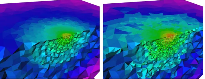
Using initial mesh with16671mesh points (for demonstration purposes), Figure 2 shows a cut
[image:14.595.193.397.92.172.2](a) Mesh at refinement level-1 (b) Mesh at refinement level-2
(c) Mesh at refinement level-3 (d) Mesh at refinement level-4
−4 −3 −2 −1 0 1 2
[image:15.595.115.447.74.203.2](e) Color scheme used for different values ofln(element size).
Figure 2: A view of meshes at different refinement levels based upon an initial mesh with16671
points.
mesh sizes (he ≈e−4) are shown by red and those with large (he≈e2) are shown by purple. One
can see that the local refinement is targeting mainly those parts of the domain close to the contact
region. However, as the refinement levels go up, the refinement also extends to the parts of the domain away from the fluid region. Moreover, Figure 2(c) shows an arc-shaped region
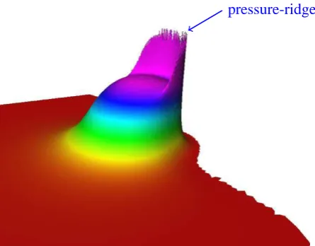
(corre-sponding to the pressure-ridge region that is present in a typical EHL solution, see Figure 3) of
the most highly-refined elements. This indicates that this is a region where the pressure-ridge affects the elastic deformation solution more significantly. Overall, this experiment (and others
pressure-ridge
Figure 3: A typical EHL solution - note the typical pressure-ridge which occurs on the outflow side of the contact.
the corresponding2D mesh for the Reynolds equation is getting finer in the region where, quali-tatively, it may be expected. A more quantitative assessment of this follows in the next subsection
(along with a comparison of different initial meshes).
4.2 Accuracy Appraisal
In this subsection, an accuracy appraisal of the different variants of the solver is considered. As a first case, the initial mesh with16671mesh points is used as the base level mesh. The EHL
problem is set up and solved on this starting mesh. Once the solution is obtained, local error
estimation on each element of the mesh is made according to equation (9) (but withΩreplaced the region occupied by elementii.e.Ωi), while a global error estimation is obtained according
to equation (10). Having the local error estimate for each element in hand, a set of elements are
marked for refinement according to equation (13). As soon as the refinement is performed, the procedure is repeated again until the maximum number of levels specified are reached (for testing
purposes the maximum refinement level is used here as stopping criterion). Recall that variant 2
of the solver also performs an optimization process on the refined meshes at each refinement level while variant 3 applies the optimization process only at the last refinement level.
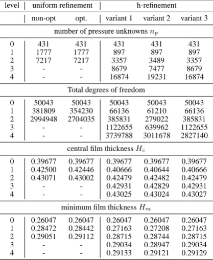
For the different mesh refinement strategies, Table 2 shows a comparison of their behaviour in
terms of problem size (both in the pressure unknowns and total problem sizes) and the solution properties (in terms of central and minimum film thicknesses). In the case of uniform (global)
refinement (optimized and non-optimized), the pressure unknowns are increasing by about a
factor of four, and the total problem size by a factor of about eight, at each level. On the other hand the local refinement process targets elements for refinement so the problem sizes grow
Table 2: Statistics for solutions using uniform refinement and adaptive h-refinement. Variant 1 performs no mesh optimization, variant 2 performs optimization at every level, and variant 3 performs optimization at the finest level only.
level uniform refinement h-refinement
non-opt opt. variant 1 variant 2 variant 3
number of pressure unknownsnp
0 431 431 431 431 431
1 1777 1777 897 897 897
2 7217 7217 3357 3489 3357
3 - - 8679 7477 8679
4 - - 16874 19231 16874
Total degrees of freedom
0 50043 50043 50043 50043 50043
1 381809 354230 66136 61210 66136
2 2994948 2704035 385831 279022 385831
3 - - 1122655 639962 1122655
4 - - 3739788 3011678 2827140
central film thicknessHc
0 0.39677 0.39677 0.39677 0.39677 0.39677 1 0.42500 0.42446 0.40666 0.40644 0.40666 2 0.43071 0.43002 0.42479 0.42482 0.42479
3 - - 0.42931 0.42829 0.42931
4 - - 0.43025 0.43024 0.43027
minimum film thicknessHm
0 0.26047 0.26047 0.26047 0.26047 0.26047 1 0.28472 0.28442 0.27163 0.27208 0.27163 2 0.29051 0.29112 0.28715 0.28744 0.28715
3 - - 0.29034 0.28947 0.29034
4 - - 0.29133 0.29121 0.29129
up the difference between the computed solution to that of uniform refinement cases becomes smaller. For example, variant 1 results in approximately the same solution after two levels of
refinement with a much smaller problem size compared to that with the uniform refinement
cases. Variant 2, which optimizes the meshes at every refinement level, seems to yield the same accuracy in results as variant 1, but with a relatively smaller problem size. Note that it was not
possible to perform a third level of uniform refinement (with or without optimization) due to
unavailability of computing resources as one can see that this would lead to a very large problem size.
It should be noted that the output of variant 3 differs from variant 1 only at the finest level due
to the additional optimization process. This optimization process leads to a significant decrease in the total size of the finest level problems while ensuring the overall accuracy of the solution.
In other words variant 3 yields the same accuracy in the solution (compared to variant 1) with
a smaller problem size at the finest level. Overall, it appears that the computed values of both Hc and Hm are converging approximately quadratically with each mesh refinement, and that
this observation holds for each variant. Furthermore the results suggest that variants 2 & 3 end
up with the same accuracy in their solution with relatively small problem sizes compared to variant 1. Indeed, we shall see next that both variants 2 & 3 result in better accuracy per degree
of freedom than both variant 1 and the uniform refinement cases.
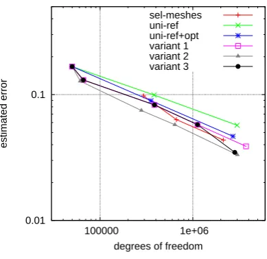
0.01 0.1
100000 1e+06
estimated error
degrees of freedom sel-meshes uni-ref uni-ref+opt variant 1 variant 2 variant 3
[image:18.595.175.370.71.260.2](a) etol= 0.2emax
Figure 4: A comparison of global error estimation using a coarsest mesh of16671points.
in Figure 4. Note that the global error estimation is for the stress, with a converging pressure
profile (different for each mesh strategy) as the traction boundary condition. The cases of uniform refinement (with and without optimization) along with the hand-tuned mesh cases (denoted
“sel-meshes”) [3] are also included. One can see that a non-optimized uniform refinement process
leads to small reduction in the (estimated) error with increasing problem size. However, if the meshes are optimized after each uniform refinement step then an improved rate of reduction in
the error is obtained. In this example, the local refinement cases (all three variants) appear to
have a superior error reduction rate, with respect to problem size, as compared to both cases of uniform refinement. It can be seen that optimization of meshes at each refinement level further
improves the rate of error reduction with respect to the problem size. It should also be noted that
the last level optimization (variant 3) significantly reduces the error at the finest level, and results in approximately the same accuracy as that obtained with the use of optimization at every level
(variant 2). Finally, the hand-tuned mesh cases perform better than the local refinement without
post-optimization of meshes (variant 1) however the automatic adaptivity with mesh smoothing does better still.
As a second test case, a different initial mesh composed of22234mesh points is considered.
Figure 5 shows the accuracy appraisal for different variants of the solver compared to the use of uniform refinement and the hand-tuned mesh cases. The same behaviour in the results can be
observed as before, however the case of optimized uniform refinement is now competitive with
the error reduction rate for the non-optimized local refinement. Nevertheless, it can again be seen that the local refinement cases (both with optimization at only the last or at every level, variants 3
0.01 0.1
100000 1e+06
estimated error
degrees of freedom sel-meshes uni-ref uni-ref+opt variant 1 variant 2 variant 3
[image:19.595.175.370.71.260.2](a) etol= 0.2emax
Figure 5: A comparison of global error estimation using a coarsest mesh of22234points.
post optimization at only the final, or at all levels, results in more accurate results per degree of freedom. Most importantly, the adaptive algorithm (with at least final level optimization) leads
to better results compared to the hand-tuned mesh cases. Indeed, the use of automatic mesh
refinement based upon ‘a posteriori’ error estimation has clearly led to better meshes than the hand-tuning approach described in [3].
10 100 1000 10000
100000 1e+06
time (sec)
degrees of freedom variant 1
variant 2 variant 3
(a) etol= 0.2emax
[image:19.595.184.361.483.646.2]Table 3: Statistics of solution at different refinement levels. Variant 1 performs no optimization, variant 2 perform optimization at every level, and variant 3 performs optimization at the finest level only.
level uniform refinement h-refinement
non-opt. opt. variant 1 variant 2 variant 3 Total nonlinear iterations
0 14 14 14 14 14
1 9 9 10 9 10
2 4 4 5 4 5
3 - - 4 3 4
4 - - 5 3 3
Average number of linear iterations per one nonlinear iteration
0 11.4 11.4 11.4 11.4 11.4
1 12 11 11.8 11.1 11.8
2 13.3 13 15.0 13.5 15.0
3 - - 15.0 12.7 15.0
4 - - 15.0 11.0 11.3
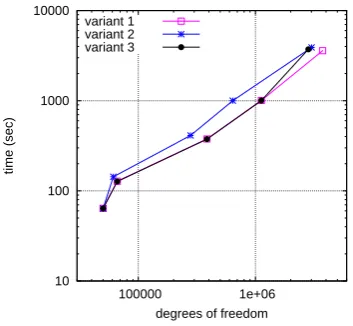
4.3 Performance
In this subsection, the CPU timings of the different variants of the proposed adaptive finite
el-ement solver are assessed. For the initial mesh case 1, the computational times are plotted in
Figure 6. Here, an initial jump in the computational time can be observed while switching from the base level to the first level. The reason is that the first refinement process led to refinement of
only a few elements meaning that the refinement overhead was relatively large (see Section 4.5
for further details). Moreover, variant 2 applies an optimization process on the refined mesh which leads to a slightly smaller problem size but the total time has increased compared to other
two variants. After the first level, the growth in the time is almost linear (i.e.O(N)) for each of
the variants, however variant 3 shows a jump in the computational time on the final level due to the optimization process on this last level mesh. Overall, the optimization of the refined meshes,
at least at the final level, leads to a relatively small change in computational time (but to relatively
more accurate results, as discussed above).
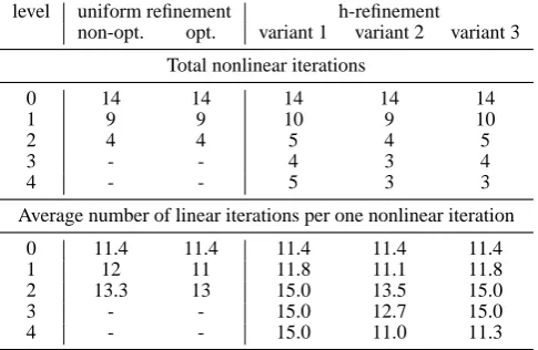
Table 3 gives statistics of average number of linear iterations and the number of nonlinear
iterations for each variant of the adaptive solver. It can be seen that as the refinement level
in-creases in each case, fewer nonlinear iterations are required to achieve convergence because of the availability of the good initial guess based upon solution at the previous level. Importantly,
the performance of the solver seems independent of the adaptivity method used. Moreover, the
optimization of meshes at final level in variant 3 results in a relatively small number of nonlinear iterations compared to variant 1. Similarly, variant 2 requires even fewer nonlinear iterations at
the intermediate levels. In addition to nonlinear iterations, variant 3 requires fewer linear
itera-tions per nonlinear iteraitera-tions at the final level while this number is also reduced for variant 2 at the intermediate levels as well.
10 100 1000 10000
100000 1e+06
time (sec)
degrees of freedom variant 1
variant 2 variant 3
[image:21.595.172.373.71.257.2](a) etol= 0.2emax
Figure 7: A comparison of performance of different variants of adaptive finite element solver using the finer initial mesh.
of the solver. Note that this observation provide another evidence that the performance of the
preconditioner [2] is optimal within this adaptive algorithm.
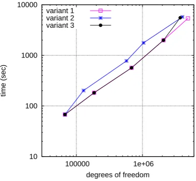
As a next case, Figure 7 shows a similar behaviour in the computational times while starting
with initial mesh case 2. No jump in the growth of time is observed on the first level due to
the refinement of a lot more elements. Again note that the optimization of refined meshes, at least at the final level, the CPU time is the same as if the meshes are not optimized. But, the
advantage of optimization of meshes is that the results thus obtained are relatively more accurate. Finally, all three variants of the solver appear to be close to optimal with approximately linear
growth in the computational time (again demonstrating the optimal performance of the multilevel
preconditioner). The qualitative behaviour of the iteration counts is similar to that shown in Table 3.
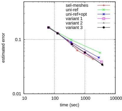
4.4 Further Discussion
In this subsection, an overall comparison between the behaviour and efficiency of different
schemes is presented. Note that all cases presented here make use of AMG preconditioning of
the elasticity block (and that geometric multigrid preconditioning is not possible for the variants of the algorithm that include the mesh optimization). Figure 8 shows a comparison of the
esti-mated global error with respect to the computational time for the different schemes considered,
using the initial mesh case 1. The hand-tuned mesh cases [3] are also included to make a com-prehensive overall comparison. It can be seen that the hand-tuned mesh cases and the different
performs just as well as the hand-tuned mesh cases. Note that each variant of the adaptive algo-rithm is fully automatic in optimizing the computational process. On the other hand, the meshes
used in the hand-tuned mesh cases are based on a large number of experiments to obtain a
de-sired accuracy at minimal cost. Furthermore, both the variants 2 & 3 of the adaptive algorithm are comparatively better than the variant 1 in reducing the overall error at a fixed computational
cost.
4.5 Accuracy of Intermediate Solves
The results presented so far were obtained by solving the nonlinear EHL problem to full
accu-racy at each refinement level. However, it is generally not necessary to solve the problem too accurately at each intermediate level. In other words, it is only necessary to solve a problem to a
sufficient precision to obtain a good approximation to the solution in order to direct the adaptive
procedure. In this subsection, the effect of different stopping tolerances for nonlinear solves at each of the intermediate levels is discussed. It should be noted that the final level problem will
always be solved to full accuracy. For this purpose, an experiment is setup using variant 3. Recall
that variant 3 only performs optimization on the refined meshes at the final level. In this experi-ment, refinement criterionetol= 0.25emaxis used. Note that, there is no specific reason for the
choice of variant 3 of the solver or the refinement criterion other than to make it a typical test. A
total of four refinement levels are used in this experiment, with initial mesh case 1 as a base level mesh. The results obtained for different stopping tolerances for the Newton solver are given in
Table 4, in terms of the number of pressure unknowns (np), the total problem size, the nonlinear iterations (ni), the linear iterations (li) and the total solve time (excluding time for optimization
at the final level), the optimization time at the final level and the global error estimation.
0.01 0.1
10 100 1000 10000
estimated error
time (sec) sel-meshes uni-ref uni-ref+opt variant 1 variant 2 variant 3
[image:22.595.172.380.475.663.2](a) etol= 0.2emax
Table 4: Effect of different stopping tolerances (U being the machine unit roundoff) for interme-diate level nonlinear solves upon the overall performance of the adaptive solver.
abstol np total dof ni li time (sec) opt-time (sec) estimated global error
U13 12835 1569053 3 36 1640 669 0.0429396
10−3
12818 1567527 3 36 1495 666 0.0429393 10−2
12768 1562842 3 34 1276 666 0.0429871 10−1
12747 1564912 3 32 1262 669 0.0429649 10−0
12323 1277703 5 61 1327 537 0.0461213
10 100 1000 10000
100000 1e+06
time (sec)
degrees of freedom abstol=U1/3
abstol=10-1
Figure 9: The effect of tolerance for the intermediate solves over the performance of an adaptive procedure.
Note that significant savings in the computational times are achieved with an increase in the
tolerance. The use of tolerance as high as10−1leads to about25%savings in the total solve time
while keeping the other values almost unchanged. A further increase in the tolerance to10−0
affects the refinement process more significantly. This tolerance results in a smaller problem with
a relatively large error. Most probably, the quality of initial guess is also not so good causing
the computational work to grow slightly compared to the 10−1 case. Hence, an intermediate
tolerance of10−1is recommended on the basis of this, and similar, tests.
Finally, Figure 9 shows the behaviour in the growth of the computational time for the accurate
and approximate solves at intermediate levels (excluding the optimization time). One can see that the jump in the computational time at the first level has not appeared in the case of the
(i−1)thlevel.
5 HEAVILY LOADED PROBLEMS
So far, the accuracy and the performance of adaptive algorithm (all three variants) has been
discussed in detail for a single moderately-loaded EHL case. The same overall performance of
the adaptive algorithm is observed for other moderately-loaded EHL test cases, for example, the caseM = 50, L= 10withph = 0.79G Pa [40] and the caseM = 200, L= 10withph = 0.97
G Pa [42], so they are not repeated here.
Heavily-loaded cases are comparatively more difficult to solve however. Some heavily-loaded cases may require under-relaxation as well as a better initial guess for the Newton procedure
to achieve convergence. Note that throughout the work presented here no under-relaxation was
used, i.e. a full Newton step was employed in the Newton procedure. However, in order to ob-tain a good performance of the adaptive procedure for more heavily-loaded cases one needs
to provide a high quality initial guess to the next refinement level. For example, if the refined
mesh following an adaptive step is not sufficiently fine then the solution of the linear elasticity equation (with interpolated pressure as traction boundary conditions) yields a better initial guess
compared to an interpolated linear elastic solution. However, once the mesh is sufficiently fine
then the interpolated linear elastic solution provides a slightly better initial guess. Moreover, for heavily-loaded EHL cases the fluid equation is advection-dominated in the contact region. Hence
starting with a very coarse initial mesh can lead to intermediate solutions with oscillatory pres-sure and may even cause failure of convergence of the Newton iteration. Note that the overall
stability of pressure solution is ensured with the use of SUPG method as described in [45] and
addition of smoothing diffusion [22] based upon the minimum of element size in a mesh. In the following subsections, accuracy and performance of proposed adaptive algorithm is
dis-cussed for a heavily-loaded case withM = 1007.6, L= 12.05andph = 2.0G Pa [41]. Based
upon the performances of different variants of the adaptive algorithm as seen in the previous sec-tion, we shall only consider the variant 2 to assess the performance of adaptive algorithm. This
choice provides similar accuracy to variant 3 but with lower overall memory requirements.
5.1 Accuracy
In this subsection, the accuracy appraisal of variant 2 of the adaptive solver is considered. The initial mesh is chosen sufficiently fine in order to obtain an acceptable starting solution. Table 5
shows a comparison against results from [41] in terms of central and minimum film thicknesses
of the solution. It is possible to see the convergence behaviour of both of the solution methods (our adaptive algorithm and method of [41]). Note that the adaptive algorithm only targets
Table 5: Validation of results of variant 2 (with c = 0.3) of adaptive finite element solver: M = 1007.6, L= 12.05andph = 2.0G Pa.
Venner [41] This model
nx×ny Hc Hm np Total dof Hc Hm
65×65 1.213×10⁻² 7
.918×10−4
− − − −
129×129 2.281×10⁻² 6
.566×10−3 4854 666160 2
.293×10−2 3
.903×10−3
257×257 2.613×10⁻²
8.975×10⁻³
6419 745902 2.453×10⁻²
7.718×10⁻³
513×513 2.690×10⁻²
9.424×10⁻³
13711 1602287 2.583×10⁻²
8.319×10⁻³
1025×1025 2.712×10⁻² 9
.594×10−3 22154 3350526 2
.656×10−2 8
.954×10−3
0.01 0.1
100000 1e+06
estimated error
degrees of freedom M1007.6-L12.05
[image:25.595.91.493.107.186.2]M20-L10
Figure 10: A comparison of global error estimation for moderately and heavily-loaded EHL cases.
level goes up both models appear to be converging to the same solution. Moreover, the difference
between the solution of two models is getting smaller as the number of refinement level grows. Note that a further refinement level would require more memory than is available on a typical
workstation for this 3D model. However, the results presented here still validate the accuracy of
the proposed algorithm for this heavily-loaded problem (and demonstrate that adaptivity permits an equivalent accuracy to the method of [41] to be reached with far fewer degrees of freedom).
Figure 10 shows a comparison of global error estimation with respect to problem size for the
moderately-loaded case (M = 20, L= 10) and heavily-loaded case (M = 1007.6, L= 12.05). It can be seen that the estimated global error for both EHL cases is reducing at the same rate
[image:25.595.164.424.214.459.2]heavily-Table 6: Statistics of solution at different refinement levels of variant 2 (withc= 0.3) of adaptive finite element solver:M = 1007.6, L= 12.05andph = 2.0G Pa.
np total dof ni avg.li time (sec) 4854 666160 15 35 1382 6419 745902 7 46 2618 13711 1602287 4 27 4533 22154 3350526 4 28 8838
1000 10000
1e+06
time (sec)
degrees of freedom variant 2
Figure 11: Performance of variant 2 (withc= 0.3) of adaptive finite element solver.
loaded EHL cases seems to be as effective as for the moderately-loaded EHL cases.
5.2 Performance
In this subsection, the CPU timing performance of variant 2 of the proposed adaptive finite element solver is assessed. Table 6 gives statistics for the number of nonlinear iterations, the
average number of linear iterations per nonlinear iteration, and computational times for variant 2
of the adaptive solver. Note that as the refinement level goes up, the availability of the good initial guess based upon solution at the previous level leads to fewer nonlinear iterations to achieve
convergence. It should be noted that for this heavily-loaded case the preconditioned iterative
solver requires slightly more linear iterations per nonlinear iteration (as expected). However, the average number of linear iterations per nonlinear iteration is still independent of the problem
[image:26.595.137.448.99.436.2]Note that, for sake of demonstration, the problem is solved accurately at each refinement level to observe the performance of the preconditioned iterative solver [2] within the adaptive
solver. The behaviour of the computational time with respect to problem size can be seen more
clearly in Figure 11. Note that the jump in the graph after the first refinement level is similar to that in Figure 6 and may be removed by using an approximate solve at the intermediate levels
(as in Figure 9). Furthermore, despite of solving the problem accurately at intermediate levels, no further jumps in the computational times are observed at later refinement levels, and the
computational time grows linearly with respect to the problem size. In other words, the optimality
of the preconditioned iterative solver [2] is still maintained with this adaptive algorithm for this heavily-loaded EHL case.
6 CONCLUSION
In this paper, an adaptive finite element solution to a fully-coupled EHL problem has been dis-cussed. A ZZ-error estimator has been used to find the local and global approximations to the
stress errors. These error estimations have been used to mark elements for refinement which
were exhibiting larger errors than a prescribed tolerance. The local refinement of the meshes was carried out using the algorithm that is described in Section 3.3, three variants of which have
been considered. The first variant applies a standard h-adaptive algorithm. The second variant
considered the post-optimization of the meshes at each refinement level in order to increase the accuracy. With the post-optimization process for the meshes, a new mesh was obtained at each
level which means that the hierarchy of meshes does not exist anymore. Thus, neither the
dere-finement nor the use of GMG based preconditioner is easily possible. Variant 3 of the adaptive solver only utilizes mesh optimization at the final level in order to avoid the possibility of
ex-cessive green elements on the2D surface mesh (which remains unchanged by the optimization
process).
The accuracy appraisal of all three variants of the solver were made using two different initial
meshes against the use of uniformly refined meshes (both optimized and non optimized) and
against the hand-tuned meshes [3]. The results showed that both the variant 2 and the variant 3 perform best in terms of accuracy. In other words, variant 2 & 3 have close resemblance with an
hr-adaptive algorithm (at least at the final level) resulting in superior results. Although
optimiza-tion of the meshes results in a loss of the nested grid property, the unchanged surface meshes allowed us to generate a high quality initial guess (by solving a linear elasticity problem with
the interpolated boundary condition) to reduce the computational work at the subsequent levels.
Moreover, all three variants of the solver show essentially linear growth in their computational time. Significantly, it is shown that an approximate solve at each of the intermediate levels leads
to a slower linear growth in the computational time.
& 3 require a slightly longer time than the variant 1 (for a fixed problem size). However, both the variants 2 & 3 of adaptive algorithm are comparatively better than the variant 1 in reducing
the overall error at a fixed computational cost. Indeed, it is demonstrated that the performance
of proposed adaptive algorithm is maintained for heavily-loaded EHL cases, with the optimality of the preconditioned iterative solver [2] being preserved despite a slight increase in the solution
times.
Perhaps the most important observation is that our computational experiments clearly
demon-strate that using the error in the stress to control the mesh adaptivity is appropriate for
fully-coupled EHL problems. The resulting adaptation of the surface mesh in the contact region allows the pressure profile to be captured accurately and with many fewer degrees of freedom than is
possible with a conventional finite difference scheme. Moreover, since stress information can
not be obtained using a surface integral solver based upon a half-space approximation, this adap-tive approach can only be applied when a finite element approximation to the linear elasticity
problem is used.
The key contributions of this work may be summarised as follows. We have introduced a new adaptive procedure for the fully-coupled EHL problem, based solely upon a local error
estimate for the stress due to the elastic deformation, and demonstrated that this provides a robust
mechanism for adapting the mesh in both the elasticity and the Reynolds discretizations. We have developed an adaptive strategy that combines h-refinement and r-refinement (node movement) in
a manner that allows locally optimal mesh refinement. The combination of local adaptivity and
our novel multigrid-based preconditioner, for the inner iterations of the Newton-Krylov solver, allow this fully-coupled EHL problem to be solved with linear time complexity for the first time:
hence providing the first demonstration of the competitiveness of the fully-coupled approach with
less general, but also optimal, half-space approximations such as [42]. Finally, and importantly, we have shown that the proposed technique is robust for heavily-loaded cases, which are by far
the most computationally challenging.
ACKNOWLEDGEMENTS
The first author thanks to Hazara University and Higher Education Commission (HEC), Pakistan for their
financial support that has allowed this research to be undertaken at the University of Leeds.
References
[1] S. Ahmed. Efficient Finite Element Simulation of Full-System Elastohydrodynamic Lubrication
Problems. PhD thesis, University of Leeds, Leeds, UK, 2012.
[2] S. Ahmed, C. E. Goodyer, and P. K. Jimack. An efficient preconditioned iterative solution of
[3] S. Ahmed, C. E. Goodyer, and P. K. Jimack. On the linear finite element analysis of fully-coupled point contact elastohydrodynamic lubrication problems. Proceedings of the Institution of
Mechani-cal Engineers, Part J: Journal of Engineering Tribology, 226(5):350–361, (2012).
[4] M. Ainsworth and J. T. Oden. A posteriori error estimation in finite analysis. John Wiley & Sons,
Inc., New York, 2000.
[5] M. Ainsworth, J. Z. Zhu, A. W. Craig, and O. C. Zienkiewicz. Analysis of the Zienkiewicz-Zhu
a-posteriori error estimator in the finite element method. International Journal for Numerical Methods
in Engineering, 28:2161–2174, 1989.
[6] T. Apel, S. Grosman, P. K. Jimack, and A. Meyer. A New Methodology for Anisotropic Mesh Refinement Based Upon Error Gradients. Applied Numerical Mathematics, 50:329–341, 2004.
[7] I. Babuska, T. Strouboulis, C. S. Upadhyay, S. K. Gangaraj, and K. Copps. Validation of a pos-teriori error estimators by numerical approach. International Journal for Numerical Methods in
Engineering, 37:1073–1123, 1994.
[8] J. Boyle, M. Mihajlovic, and J. Scott. Hsl mi20: An efficient amg preconditioner for finite element
problems in 3d. International Journal for Numerical Methods in Engineering, 82(1):64–98, 2010.
[9] A. Brandt and A. A. Lubrecht. Multilevel Matrix Multiplication and Fast Solution of Integral
Equa-tions. Journal of Computational Physics, 90(2):348–370, 1990.
[10] W. L. Briggs, V. E. Henson, and S. F. McCormick. A Multigrid Tutorial. Society for Industrial and
Applied Mathematics, 2000.
[11] A. N. Brooks and T. J. R. Hughes. Streamline-upwind/petrov-galerkin formulations for convective
dominated flows with particular emphasis on the incompressible navier-stokes equations. Comp. Meth. Appl. Mech. Engnrg, Vol. 32:pp.199–259, 1982.
[12] T. A. Davis. Algorithm 832: Umfpack, an unsymmetric-pattern multifrontal method. ACM
Trans-actions on Mathematical Software, 30(2):196–199, June 2004.
[13] D. Dowson and G. R. Higginson. Elastohydrodynamic Lubrication. Pergamon Press, Oxford, 1977.
[14] H. G. Elrod. A Cavitation Algorithm. Journal of Lubrication Technology-Transactions of the ASME, 103:350–354, 1981.
[15] H. P. Evans and T. G. Hughes. Evaluation of Deflection in Semi-Infinite Bodies by a Differential
Method. Proceedings of the Institution of Mechanical Engineers, Part C: Journal of Mechanical
Engineering, 214:563–584, 2000.
[16] L. Floberg. Cavitation in Lubricating Oil Films. Elsevier, Amsterdam, 1964.
[17] C. E. Goodyer. Adaptive Numerical Methods for Elastohydrodynamic Lubrication. PhD thesis,
University of Leeds, Leeds, UK, 2001.
[18] C. E. Goodyer and M. Berzins. Adaptive timestepping for elastohydrodynamic lubrication solvers.
SIAM Journal on Scientific Computing, 28:626–650, 2006.
[19] C. E. Goodyer and M. Berzins. Parallelization and scalability issues of a multilevel
[20] W. Habchi. A Full-System Finite Element Approach to Elastohydrodynamic Lubrication Problem: Application to Ultra-Low-Viscosity Fluids. PhD thesis, University of Lyon, France, 2008.
[21] W. Habchi, D. Eyheramendy, P. Vergne, and G. Morales-Espejel. A full-system approach of the elastohydrodynamic line/point contact problem. ASME Journal of Tribology, 130(2), 2008.
[22] W. Habchi, D. Eyheramendy, P. Vergne, and G. Morales-Espejel. Stabilized Fully-Coupled Finite El-ements for elastohydrodynamic Lubrication Problems. Advances in Engineering Software, 46(1):4–
18, 2012.
[23] M. J. A. Holmes, H. P. Evans, T. G. Hughes, and R. W. Snidle. Transient Elastohydrodynamic
Point Contact Analysis Using a New Coupled Differential Deflection Method. Part I: Theory and
Validation. Proceedings of the Institution of Mechanical Engineers, Part J: Journal of Engineering
Tribology, 217:289–303, 2003.
[24] M. J. A. Holmes, H. P. Evans, T. G. Hughes, and R. W. Snidle. Transient Elastohydrodynamic Point
Contact Analysis Using a New Coupled Differential Deflection Method. Part II: Results.
Proceed-ings of the Institution of Mechanical Engineers, Part J: Journal of Engineering Tribology, 217:305– 321, 2003.
[25] L. G. Houpert and B.J. Hamrock. Fast approach for calculating film thicknesses and pressures in elastohydrodynamically lubricated contacts at high loads. ASME Journal of Tribology, Vol 108:pp.
411–420, 1986.
[26] T. G. Hughes, C. D. Elcoate, and H. P. Evans. Coupled Solution of the Elastohydrodynamic Line
Contact Problem Using a Differential Deflection Method. Proceedings of the Institution of
Mechan-ical Engineers, Part C: Journal of MechanMechan-ical Engineering, 214:585–598, 2000.
[27] R. Lohner and J. D. Baum. Adaptive h-refinement on 3d unstructured grids for transient problems.
International Journal for Numerical Methods in Fluids, 14:1407–1419, 1992.
[28] H. Lu. High Order Finite Element Solution of Elastohydrodynamic Lubrication Problems. PhD
thesis, University of Leeds, Leeds, UK, 2006.
[29] A. A. Lubrecht. Numerical solution of the EHL line and point contact problem using multigrid
techniques. Phd thesis, University of Twente, Endschende, The Netherlands, 1987.
[30] R. Mahmood and P. K. Jimack. Locally optimal unstructured finite element meshes in 3 dimensions.
Computers and Structures, 82:2105–2116, 2004.
[31] J. E. Marsden and T. J. R. Hughes. Mathematical Foundations of Elasticity. Dover Publications,
Inc., New York, 1994.
[32] M. Moller and D. Kuzmin. Adaptive mesh refinement for high-resolution finite element schemes. International Journal for Numerical Methods in Fluids, 52(5):545–569, 2006.
[33] K. P. Oh and S. M. Rohde. Numerical solution of the point contact problem using the finite element method. International Journal for Numerical Methods in Engineering, Vol 11:pp. 1507–1518, 1977.
[34] H. Okamura. A contribution to the numerical analysis of isothermal elastohydrodynamic lubrication. Proc. 9th Leeds-Lyon Symp. Trib., 1982(Leeds, UK).
![Table 1: Non-dimensional parameters for the contact between steel surfaces [42].](https://thumb-us.123doks.com/thumbv2/123dok_us/7920320.191569/14.595.193.397.92.172/table-non-dimensional-parameters-contact-steel-surfaces.webp)