Rician statistical assumptions for geographic routing in wireless sensor networks

wireless sensor networks.

White Rose Research Online URL for this paper: http://eprints.whiterose.ac.uk/92870/

Version: Accepted Version

Article:

Popescu, AM, Salman, N and Kemp, AH (2015) Rician statistical assumptions for

geographic routing in wireless sensor networks. IET Wireless Sensor Systems, 5 (4). pp. 204-209. ISSN 2043-6386

https://doi.org/10.1049/iet-wss.2014.0023

[email protected] https://eprints.whiterose.ac.uk/ Reuse

Unless indicated otherwise, fulltext items are protected by copyright with all rights reserved. The copyright exception in section 29 of the Copyright, Designs and Patents Act 1988 allows the making of a single copy solely for the purpose of non-commercial research or private study within the limits of fair dealing. The publisher or other rights-holder may allow further reproduction and re-use of this version - refer to the White Rose Research Online record for this item. Where records identify the publisher as the copyright holder, users can verify any specific terms of use on the publisher’s website.

Takedown

If you consider content in White Rose Research Online to be in breach of UK law, please notify us by

On Rician statistical assumptions for geographic

routing in WSNs

Ana Maria Popescu, Naveed Salman, Andrew H. Kemp,

School of Electronic and Electrical Engineering, University of Leeds, UK, LS29JT

{elamp, elns, a.h.kemp}@leeds.ac.uk

Abstract

Geographic routing algorithms for wireless sensor networks (WSNs) need to be resilient to the inherent location

errors of positioning systems. Proposed forwarding algorithms in the literature make use of the statistical assumption

of Gaussian distributed location error and Ricianly distributed distance estimates between sensor nodes. This letter

analyses the validity of the Rician hypothesis when realistic localisation is employed and simulated. We consider

received signal strength based (RSS) localisation through the linear least square method (LLS). Anchor nodes

estimate the position of the target sensor nodes as well as their error characteristics, which are no longer assumed

Gaussian. Both theoretical and simulation results confirm that the Rician assumption is not true when realistic

localisation scenarios are used, affecting the performance of geographic routing algorithms based on this statistical

supposition.

Index Terms

geographic routing algorithm, Rician assumptions, wireless sensor networks, LLS-RSS localisation

I. INTRODUCTION

A very high number of position based routing algorithms are not designed to cope with location error

and consider the location of nodes to be exactly known. In realistic wireless sensor networks (WSNs)

with hundreds of nodes, this assumption is not valid, as these nodes are localised using local positioning

systems [1], [2], [3]. Localised nodes have a specific error associated with them, whose magnitude differs

depending on the employed ranging technique. Location error values are random in reality and their

variance for the x and y coordinates may or may not be the same. No physical environmental factors are considered here that may affect their values (i.e. wind currents), but differences may still exist, because of

of the routing procedure [4]. Thus, efficient geographic routing algorithms have to be able to cope with

location errors [5], [6], [7], [8].

The widely used mathematical error model considers location errors normally distributed [5], [6], [7],

[8], which facilitates the assumption that the distances between nodes have a Rice distribution. The Rice

statistical statement is possible only if a simplifying assumption is made i.e. the variance of the estimated

x and y coordinates is equal. However, this is not necessarily always true and can affect the forwarding

algorithms if based on Rician assumptions. This work presumes the Rician hypothesis true and verifies

it via MATLAB simulations, when employing a realistic localisation simulation (here based on received

signal strength (RSS) ranging).

The paper is organized as follows: Section 2 briefly lists some of the most significant sensor network

localisation methods used in WSNs and presents error-coping geographic routing algorithms which suffer

from the Rician distribution assumption. Section 3 discusses the problem of the Rician assumption in the

design of geographic routing algorithms. Section 4 describes three simulation tests performed as part of

a preliminary analysis to confirm the existence of the theoretical issue. Non-Rician geographic routing

solutions are presented in Section 5 and comparatively analysed via simulations in Section 6. Conclusions

are drawn in Section 7.

II. RELATED WORK

Geographic routing is an attractive option for large scale WSNs, because of its low overhead and

energy expenditure, but is inefficient in realistic localisation conditions which are inevitably imprecise.

Inexact range measurements and location errors can lead to low throughput and to node power being

wasted. Accurate localisation is therefore essential in position-based routing for WSNs. According to

the position knowledge, sensor nodes can be divided into two categories: anchors (or beacon nodes) and

targets (or blindfolded nodes). Anchor positions are usually known with accuracy (either through the global

positioning system (GPS) or installation measurements). GPS use is however economically unjustifiable

for each node in a large or inaccessible network. The coordinates of target nodes can alternatively be

estimated using localisation algorithms, the absolute positions of the anchors and inter-sensor node range

measurements. Measurement techniques can be classified as based on angle (angle of arrival (AoA)),

distance (one way or two way time of arrival (OW-ToA or TW-ToA), time difference of arrival (TDoA),

is chosen over others because it is suitable for smaller networks and allows fast simulation processing.

However, possible future work can make use of other methods of localisation.

While, the most forward within range (MFR) algorithm [10] is an example of a geographic routing

algorithm which does not cope with location errors, recent literature does provide a few solutions to cope

with inaccurate location errors in an energy efficient way. MFR is also considered an energy efficient

forwarding strategy when using a fixed transmission power, because it minimizes the hop count [5], but

it has been proven less efficient than other routing algorithms in realistic WSN conditions.

The least expected distance algorithm (LED) is proposed in [6]. It is presented as an error-robust routing

scheme, whose main aim is to preserve the power saving features of basic geographic forwarding. It is

proven in [6] that whichever approach the position-based routing may have, either to optimize the energy

spent per hop or for the overall chosen path, there is a unique energy-optimal forwarding position which

can be used in the forwarding process. LED determines this theoretical optimum and chooses as a next

hop the neighbour whose real position is closest to it. The algorithm strategically incorporates location

error into the forwarding objective function. It is assumed that the estimated coordinates of each node

are affected by a Gaussian error of a given variance. As a consequence, the erroneous distances between

nodes are random variables characterized by the Rice distribution. LED calculates the expectation of the

considered distances and chooses the node with the minimum expectation.

The mean square error ratio (MSER) and the conditioned mean square error ratio (CMSER) algorithms

are proposed in [8] as alternative methods for geographic routing resilient to location errors. MSER

represents the basic forwarding strategy, while CMSER represents a better developed version of the

algorithm. Both MSER and CMSER make use of the notion of maximum advance to destination

(just as MFR), but consider the probability of a successful packet transmission when coordinates are

affected by location error. The algorithms are analysed via simulation using different network sizes, error

characteristics and communication ranges and all results confirm the expected performance of CMSER

in terms of both throughput and energy savings. As does LED, MSER and CMSER make use of initial

Gaussian error assumptions and of Ricianly distributed distances.

Geographic routing algorithms which cope with inaccurate position knowledge of the nodes are based

on a chain of statistical assumptions, amongst which, one is that of equality of the location error variance

assumption of distance estimates to be valid. However, if the theoretical calculations or the simulation

results of these statistics are not the same (or not assumed to be the same) then node distances may also

not be Ricianly distributed. Consequently, the routing algorithms using this assumption may not perform

optimally either. This is studied further in the following sections.

III. PROBLEM STATEMENT

Efficient geographic routing algorithms for WSNs are designed to cope with inaccurate localisation

[5], [6], [7], [8]. The widely used mathematical error model considers the distance estimate between two

localised nodes as a random variable (RV) with a Rician distribution. The estimated distance between

node i and j is given by

ˆ

dij =

√

X2 +Y2

,

where X and Y are represented by (ˆxi−xˆj) and (ˆyi−yˆj) and where (ˆxi,yˆi) and (ˆxj,yˆj) are the

estimated location coordinates of nodes i and j respectively. The distance dˆij Ricianly distributed i.e.

fdˆij

= dˆij

σ2 ij

!

exp

 −

ˆ

dij 2

+d2 ij 2σ2

ij

 I0

ˆ

dijdij σ2

ij

!

. (1)

The distribution of the difference of two normally distributed variates, (ˆxi−xˆj) or (ˆyi−yˆj), is also

Gaussian with mean µij =µi−µj and variance σ 2 ij =σ

2 i +σ

2

j. dˆij can be a Rician RV only if X and Y

have the same variance σ2

ij. This is the equivalent of the variance in any nodei orj being the same on the xandyaxes:σ2

ix =σ 2

iy(referred to as σ 2

i) andσ 2 jx =σ

2

jy (referred to asσ 2

j). Such a statistical presumption

is a simplification, which in reality is not always true and can affect the forwarding algorithms based on

Rician assumptions.

It is considered that the target sensor nodes (TN) are randomly distributed in the network having a

location error model as described above. Anchor nodes (AN) estimate the position of the target sensor

nodes and their error characteristics. Received signal strength (RSS) ranging is used for localisation and

simulated using the linear least square method (LLS) as in [1]. Following [1], the error variance associated

with each node i is theoretically estimated using the trace of the covariance matrix:

where θˆ_{i =}    ˆ xi ˆ yi  

 represents the estimated location via LLS, θi =    xi yi  

represents the true location

coordinates and Covˆθ_{i is the covariance matrix:}

Covθˆ_i=Ehθˆ_i−θ_i θˆ_{i −}θ_iTi ₍₃₎

=E       ˆ

xi−xi ˆ

yi−yi

  

ˆ

xi−xi yˆi−yi

   =E   

(ˆxi−xi) 2

(ˆxi−xi)(ˆyi−yi) (ˆyi−yi)(ˆxi −xi) (ˆyi−yi)

2    =   

E[(ˆxi−xi) 2

] E[(ˆxi−xi)(ˆyi−yi)] E[(ˆyi−yi)(ˆxi−xi)] E[(ˆyi −yi)

2 ]

  .

The main diagonal terms of of the matrix in Eq. 3 represent the theoretical variance of the location error

on the x and y axes:

σ2 ix =E

h

(ˆxi−xi) 2i

, (4)

σ2 iy =E

h

(ˆyi−yi) 2i

, (5)

and the terms in the off-diagonal represent the covariance between the x and y location error (for

referenceσxy) and, if the RVs are independent,

E[(ˆxi−xi)(ˆyi−yi)] =E[(ˆyi −yi)(ˆxi−xi)] = 0.

The calculation of the theoretical MSE from Eq. 2 is presented in detail in [1]. The simulation of

the LLS-RSS localisation takes place with a prescribed noise value srss [dB] reflected in the distance

variance [m2_{]. Environmental interference is taken into account only by the localisation simulations (whose}

ranging is affected by assumed noise values). It is not considered in the simulation of the routing process.

Although this is a simplification, it does not affect the scope of the work. The localisation simulation

2, σ2

RSS =σ 2 ix +σ

2

iy. If the distances are assumed Ricianly distributed, then σ 2 ix =σ

2 iy =

σ2

RSS

2 . The aim

is to show that σ2 ix 6= σ

2

iy, to analyse the impact of this inaccurate assumption on geographic routing

performance and to propose more accurate forwarding alternatives.

IV. PRELIMINARY ANALYSIS

To verify whether the location variance of random nodes i is actually the same for the x and y

coordinates, for the RSS technique, three tests are used. The randomly deployed TNs are localised through

LLS-RSS by the ANs, placed at the edge of the square network (with sidel= 50[m]). The communication range R = 10 [m] is the same for all the TNs, while the transmission range of the ANs covers the entire network surface. The localisation process is simulated assuming different values for the path loss exponent

(PLE) α [dB] and η iterations are considered for averaging.

The variance of the location error of the nodes is influenced only by the number and position of the

anchors nodes. The number of target nodes is not relevant, but their position in regards to the anchor

nodes is. For example, the coordinates of a centrally placed target node, which is equally far from all

anchor nodes, will be estimated with more precision than a target node which is closer only to few anchor

nodes.

• Test 1: Comparison via simulation samples

A network of T N = 30 and AN = 9 is used for the simulation (ANs are placed on the edges, in the corners and in the center of the network) (α= 2.5). Random nodesiare selected and a comparison is made between the average variance value resulting from the RSS localisation process, using σ2RSS

2 (averaged over

η = 100), and the estimated values of σ2

ix and σ 2

iy, calculated using V ar(X) =E[(X−E(X)) 2

], where

X is represented by the erroneous coordinates of node i whose values are different for each iteration and

E(X) is the mean of X, which should be the actual coordinates of node i. Table I: Results for Test 1

T N l srss σ2

RSS

2 σ 2 ix σ

2 iy

4 100 0.6 37.69 27.82 23.93 10 100 0.6 44.00 32.71 33.89

4 100 1 63.25 46.10 40.02

25 50 1 7.84 5.01 6.71

2 50 0.6 9.61 8.87 9.62

27 50 0.6 6.72 5.25 6.43

3 50 1.5 12.48 15.89 8.88

The results of this initial test show σ2 ix 6=σ

2

iy and that the RSS calculated variance is an approximation

(an example is presented in Table I). As the σ2RSS

2 value is an estimation, its accuracy depends on the TN

position referenced to the ANs and on the network size (RSS ranging is not suitable for large networks

[1], [11]). The values for σ2

ix and σ 2

iy which are obtained through theoretical calculations are similar, but

not equal.

• Test 2: Network visualization comparison

This test aims to illustrate the location error of the nodes, when estimated with equal or different variance

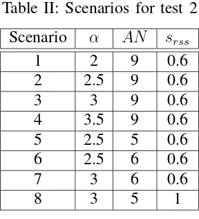
for the xand y coordinates. The simulations consider T N = 10 and η= 100 and the employed scenarios are listed in Table II. Using the LLS-RSS localisation, the variations are made for α, the number and positions of the AN s and for the noise value srss.

Table II: Scenarios for test 2

Scenario α AN srss

1 2 9 0.6

2 2.5 9 0.6

3 3 9 0.6

4 3.5 9 0.6

5 2.5 5 0.6

6 2.5 6 0.6

7 3 6 0.6

8 3 5 1

The values of σ2

ix and σ 2

iy are calculated for each node i and compared with the values σ2

RSS

2 obtained

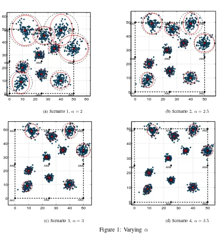
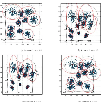
from the simulation. The black dashed circles in the figures represent the area where the estimated positions

of the nodes are considered to be when σ2 ix =σ

2

iy (centered on the accurate location of node i, of radius σ2

RSS

2 ). The red ellipses in the figures represent the areas of the estimated positions whenσ 2 ix 6=σ

2

iy (centred

is the accurate location of node i, with ellipse axes σ2 ix, σ

2 iy).

Aside from facilitating the possibility to observe the difference in the area covered by the circles and

that of the ellipses, the scenarios 1, 2, 3 and 4 in Fig. 1 illustrate how a larger α makes the location estimation more accurate (notice the decreased area of both the ellipses and the circles). Fig. 2 shows the

influence of the anchor positions on the localisation process. By reducing the number of the anchors and

removing them from the middle of the edge (scenarios 5 and 8), the localisation loses from its overall

accuracy, but not as much as when eliminating anchors from key positions, such as all the ones on the

north side of the network, affecting the localisation especially in this region (scenarios 6 and 7). While

mostly the nodes on the north side that are affected by the change and their error ellipses are particularly

larger and more elongated.

0 10 20 30 40 50 60 0

10 20 30 40 50 60

AN1 AN2 AN3

AN4 AN5 AN6

AN7

AN8 AN9

(a) Scenario 1,α= 2

0 10 20 30 40 50 0

10 20 30 40 50

AN1 AN2 AN3

AN4 AN5 AN6

AN7

AN8 AN9

(b) Scenario 2,α= 2.5

0 10 20 30 40 50 0

10 20 30 40 50

AN1 AN2 AN3

AN4 AN5 AN6

AN7

AN8 AN9

(c) Scenario 3,α= 3

0 10 20 30 40 50 0

10 20 30 40 50

AN1 AN2 AN3

AN4 AN5 AN6

AN7

AN8 AN9

(d) Scenario 4,α= 3.5

Figure 1: Varying α

In this study it has been assumed that the location errors on the x and y axes are independent and

therefore uncorrelated. Consequently their covariance is zero and the minor and major axes of the

error-ellipses are parallel to the x and y axes. However, in reality, the error on the two axes may be correlated

to a degree (as the LLS-RSS localisation process shows) and this would imply a rotation of the error

0 10 20 30 40 50 60 0

10 20 30 40 50 60

AN1 AN2

AN3 AN4

AN5

(a) Scenario 5,α= 2.5

0 10 20 30 40 50 0

10 20 30 40 50 60 70

AN1 AN2 AN3

AN4

AN5 AN6

(b) Scenario 6,α= 2.5

0 10 20 30 40 50 0

10 20 30 40 50

AN1 AN2 AN3

AN4

AN5 AN6

(c) Scenario 7,α= 3

0 10 20 30 40 50 0

10 20 30 40 50

AN1 AN2

AN3 AN4

AN5

(d) Scenario 8,α= 3

Figure 2: Varying the anchor node placement and the noise values

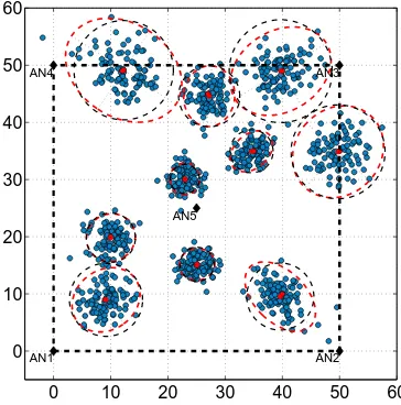
In Fig. 3, where α = 3 and srss = 0.6, the lengths of the ellipse axes are equal to the square roots

of the eigenvalues λ of the covariance matrix Covˆθ_{i in Eq. 3. The eigenvalues are calculated using}

Covˆθ_{i∗v =λ∗v, where v is the eigenvector of Cov}ˆθ_{i. The counter-clock angle of rotation of the}

ellipses is determined with

φ= 1

2arctan

2σxy

(ˆxi−xi)2−(ˆyi−yi)2

!

where (ˆxi −xi) 2

−(ˆyi−yi) 2

6

= 0. Fig. 3 illustrates another example of an unrealistic assumption in

algorithmic design.

0 10 20 30 40 50 60 0

10 20 30 40 50 60

AN1 AN2

AN3 AN4

AN5

Figure 3: Network example with correlated errors for the x and y coordinates

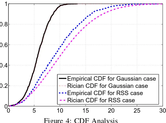
• Test 3: Cumulative distribution function comparison

It is considered that T N = 2, AN = 9 and α = 2.5. The distance between TNs is a multivariate RV (depending on the σ2

of both coordinates of two TNs). So, the cumulative distribution function (CDF),

FX(x) = 1−Q1( dij

σij,

ˆ dij

σij), where Q1 is the Marcum Q-function, can be used to verify the non-Rician

hypothesis for the LSS-RSS localisation resulted errors.

Firstly, the location error of two TN is considered Gaussianly distributed, so σ2 i 6= σ

2

j and σ 2 ix = σ

2 iy

and σ2 jx = σ

2

jy. Both the theoretical as well as the empirical Rician CDFs are computed, the empirical

CDF using simulation-obtained estimated distances dˆij, forη = 1000.

Secondly, the theoretical and empirical Rician CDFs are calculated for the same nodes, when these are

located through LLS-RSS. The estimated dˆij are taken from the ANs, which perform the ranging over

the same η as before. To calculate the scale parameterσij, the theoretical Rician CDF (for the RSS case)

assumes σ2 ix =σ

2

iy and σ 2 jx =σ

2

jy . The CDFs can be seen in Fig. 4.

For the TNs with Gaussian errors and an equal variance on both x and y axes, the theoretical and

empirical CDFs overlap as a confirmation that the distances are Ricianly distributed. For RSS estimated

node coordinates and variances, it is not accurate to assume the error variance is equal on thexandyaxes.

The difference in the CDF curves shows that such an assumption would implicitly lead to a suboptimal

0 5 10 15 20 25 30 0 0.2 0.4 0.6 0.8 1

Empirical CDF for Gaussian case Rician CDF for Gaussian case Empirical CDF for RSS case Rician CDF for RSS case

Figure 4: CDF Analysis

V. NON-RICIAN GEOGRAPHIC ROUTING SOLUTION

Two new algorithms are proposed, non-Rician mean square error ratio (NR-MSER) and non-Rician

conditioned mean square error ratio (NR-CMSER), adaptations of the MSER and CMSER algorithms

proposed in [8]. The forwarding is made on the same principles as before, but the algorithms are adapted

to cope with the difference in the x and y location error; they no longer use the Rician expectation and

variance in their calculations.

In [8], the MSER and CMSER algorithms use the mean square error (MSE):

M SEij =E

ˆ

dij −dij

₂ =E ˆ dij 2

−2dijE

ˆ

dij

+d2

ij, (6)

where dij and dˆij are the real and the estimated distance between two nodes i and j. The calculation of

the M SEij is made with the help of the Rician mean E

ˆ

dij

. Here, the mean is assumed equal to the

actual distance, Edˆij

=dij, and the mathematical expression of the MSE in Eq. 6 changes into:

N R M SEij =E

ˆ

dij 2

−d2

ij, (7)

E

ˆ

dij 2

is calculated using the Euclidean distance equation,dˆij 2

= (ˆxi−xˆj) 2

+(ˆyi−yˆj) 2

, and the second

moments which are: E(ˆx2 i) = x

2 i +σ

2

ix, E(ˆy 2 i) = y

2 i +σ

2 iy, E

ˆ

x2 j

= x2 j +σ

2

jx and E

ˆ

y2 j

= y2 j +σ

2 jy. Therefore, E ˆ dij 2

=Exˆ2

i −2ˆxixˆj+ ˆx 2 j + ˆy

2

i −2ˆyiyˆj+ ˆy 2 j

=E(ˆx2

i) +E(ˆx 2

j) +E(ˆy 2

i) +E(ˆy 2

j)−2E(ˆxixˆj)−2E(ˆyiyˆj)

=σ2 ix +σ

2 iy+σ

2 jx+σ

2 jy+x

2 i +x

2 j +y

2 i +y

2

j −2xixj −2yiyj. (8)

In Eq. 7, because dij is not known, dˆij is used in simulations instead. Similarly to [8], the mean square

error ratio (MSER) is calculated using Eq. 9. For a balanced selection of the forwarding node, NR-MSER

makes its decision by minimizing the MSE and maximizing the distance betweeniandj (the maximization of dˆij is also used by the most forward within range algorithm (MFR) [10], which is used in Section V

for comparison):

N R M SERij =N R M SEij/dˆij. (9)

Fj = arg min (N R M SERij). (10)

The NR-CMSER also makes use of an additional, modified condition. With CMSER the routing selection

was refined through: R₋dˆij

2

> V ardˆij

, where V ardˆij

is the Rician variance of the estimated

distance. However, because the Rician assumption is considered incorrect, V ardˆij

is replaced for the

NR-CMSER with the sum of the average variance in the x and y coordinates of the two nodes i and j,

(R₋dˆij) 2

> σ

2 ix+σ

2 iy

2 +

σ2 jx+σ

2 jy

2 . (11)

VI. SIMULATIONS AND RESULTS

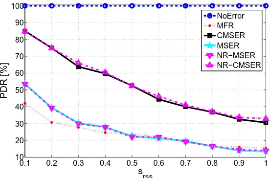
The PDR of NR-MSER and NR-CMSER is compared with their Rician-based algorithmic counterparts.

The behavior of the MFR algorithm is included in the comparison because its distance metric is used by

the other algorithms. The MFR throughput, with and without an assumed location error, is shown as a

lower and upper bound on the routing performance. All simulations are based on LLS-RSS localisation.

MSER and CMSER make use of inaccurate Rician assumptions and, unaware of a difference between

the x and y error of node i, use σ2 ix =σ

2 iy =

σ2

RSS

2 in their decisions. The provided solutions, NR-MSER

and NR-CMSER, are designed to cope with σ2 ix 6= σ

2

iy and are expected to perform the same or better

than MSER and CMSER. The packet delivery ratio (PDR) is analysed for η= 1000, l = 50, T N = 200,

increasing values of the srss.

For the smallest value of srss = 0.1, the highest PDR is reached, 54% for MSER and NR-MSER and

85% for CMSER and NR-CMSER. As srss is increased, reaching the value of 1, the routing performance

for all algorithms degrades to such a level that the PDR becomes 15% for MSER and NR-MSER or 30%

for CMSER and NR-CMSER. In Fig. 5 the PDR of the non-Rician algorithms remains approximately the

same as that of the Rician ones. Because one would expect a bigger difference in routing performance,

it is considered that the routing performance may be affected only by a large difference in σ2

ix and σ 2 iy.

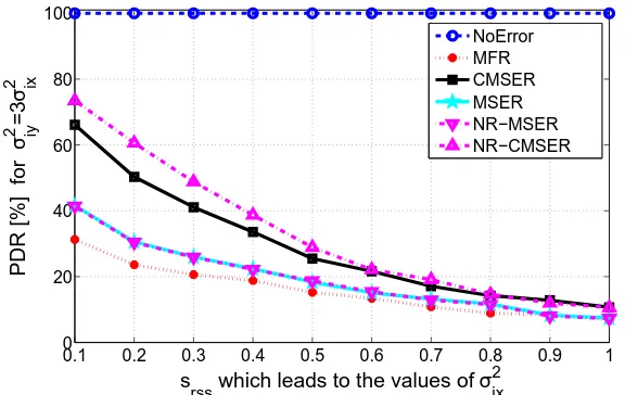
Such a scenario may exist and the large difference in the x and y variance may be undetected by the

localisation system, depending on its method of estimation, accuracy, number of anchors and network

area. This possibility is tested in Fig. 6.

0.1 0.2 0.3 0.4 0.5 0.6 0.7 0.8 0.9 1 10

20 30 40 50 60 70 80 90 100

s

rss

PDR [%]

NoError MFR CMSER MSER NR−MSER NR−CMSER

Figure 5: Performance based on RSS localisation

The difference in the x and y error is increased “artificially” by considering σ2 ix =

σ2

RSS

2 as obtained

from the LLS-RSS localisation process and σ2 iy= 3σ

2

ix. MSER and CMSER are unaware of this difference

(all according to the hypothesis that the localisation method does not reflect accurately the difference in

the actual error on the x and y axes) and still use σ2 ix = σ

2 iy =

σ2

RSS

2 . In this new scenario (from Fig.

6), although the PDR for all algorithms is smaller, the NR-CMSER algorithm performs better. The test

illustrates that only large differences in σ2

ix and σ 2

iy reveal the improvement of the new algorithms.

Overall, the performance of the new algorithms is either the same or better than the unadjusted

counterparts and most importantly, NR-MSER and NR-CMSER are formulated correctly and cope with

0.1 0.2 0.3 0.4 0.5 0.6 0.7 0.8 0.9 1 0

20 40 60 80 100

s

rss which leads to the values of σix 2

PDR [%] for

σ iy 2 =3

σ ix

2

NoError MFR CMSER MSER NR−MSER NR−CMSER

Figure 6: Performance based on RSS resulted σ2

ix, but with large σ 2 iy

VII. CONCLUSIONS

Analysis through the above described methods proves the Rician assumption is not valid when sensor

nodes are located through realistic localisation methods (RSS or otherwise), because the error variance

in the x and y coordinates of a node may not be the same (as the Rician assumption implies). While

algorithms based on the Rician hypothesis can perform well in simulations, their results are not realistic

and their performance can be affected by a large difference in the x andy error. The proposed geographic

routing solutions NR-MSER and NR-CMSER realistically forward data, while coping with location error,

without making use of the Rician assumption.

REFERENCES

[1] Salman, N., Ghogho, M., Kemp, A.H., “Optimized Low Complexity Sensor Node Positioning in Wireless Sensor Networks”, Sensors

Journal, IEEE, vol. 14, Issue 1, 2014, pp. 39 - 46Rasool, I., Kemp, A.H., “Statistical analysis of wireless sensor network Gaussian

range estimation errors”, IET Wireless Sensor Systems, vol. 3, Issue 1, 2013, pp. 57 – 68

[2] Rasool, I., Kemp, A.H., “Statistical analysis of wireless sensor network Gaussian range estimation errors”, IET Wireless Sensor Systems,

vol. 3, Issue 1, 2013, pp. 57 – 68

[3] Moussakhani, B., Flåm, J.T., Støa, S., Balasingham, I., Ramstad T., “On localisation accuracy inside the human abdomen region”, IET

Wireless Sensor Systems, vol. 2, Issue 1, 2012, pp. 9 – 15

[4] Yu, R., Zhang Y., Yang, K., Xie S., Chen 4, H.-H., “Distributed geographical packet forwarding in wireless sensor and actuator networks

– a stochastic optimal control approach”, IET Wireless Sensor Systems, vol. 2, Issue 1, 2012, pp. 63 – 74

[5] Kwon, S., Shroff, N.B., “Geographic routing in the presence of location errors”, Computer Networks (2006), vol.50, pp.2902-2917.

[6] Peng, B., Kemp, A.H., “Energy-efficient geographic routing in the presence of location errors”, Computer Networks (2011), vol.55,

[7] Marin-Perez, R., Ruiz, P.M., “Effective Geographic Routing in Wireless Networks with Inaccurate Location Information”, In Proceedings

of the 10th International conference on Ad-hoc, mobile, and wireless networks (ADHOC-NOW’11), Paderborn, Germany, 2011, pp.1-14

[8] Popescu, A.M., Salman, N., Kemp, A.H., “Geographic Routing Resilient to Location Errors”, Wireless Communications Letters, IEEE,

2013, vol.2, no.2, pp.203-206

[9] Mao, G., Fidan, B., Anderson, B.D.O., “Wireless sensor network localization techniques”, Computer Networks, 2007, pp. 2529 - 2553.

[10] Takagi H., Kleinrock L., “Optimal transmission range for randomly distributed packet radio terminals”, IEEE Transactions on

Communications 32 (3), 1984, pp.246-257.

[11] Patwari, N. Hero, A. O., “Using Proximity and Quantized RSS for Sensor localization in Wireless Networks”, Proceedings of the 2nd