A Bayesian non-linear method for feature selection in machine translation quality estimation

translation quality estimation

.

White Rose Research Online URL for this paper:

http://eprints.whiterose.ac.uk/98286/

Version: Accepted Version

Article:

Shah, K., Cohn, T. and Specia, L. orcid.org/0000-0002-5495-3128 (2015) A Bayesian

non-linear method for feature selection in machine translation quality estimation. Machine

Translation, 29 (2). pp. 101-125. ISSN 0922-6567

https://doi.org/10.1007/s10590-014-9164-x

[email protected] https://eprints.whiterose.ac.uk/ Reuse

Unless indicated otherwise, fulltext items are protected by copyright with all rights reserved. The copyright exception in section 29 of the Copyright, Designs and Patents Act 1988 allows the making of a single copy solely for the purpose of non-commercial research or private study within the limits of fair dealing. The publisher or other rights-holder may allow further reproduction and re-use of this version - refer to the White Rose Research Online record for this item. Where records identify the publisher as the copyright holder, users can verify any specific terms of use on the publisher’s website.

Takedown

If you consider content in White Rose Research Online to be in breach of UK law, please notify us by

(will be inserted by the editor)

A Bayesian non-Linear Method for Feature Selection

in Machine Translation Quality Estimation

Kashif Shah · Trevor Cohn · Lucia

Specia

Received: date / Accepted: date

Abstract We perform a systematic analysis on the effectiveness of features for

the problem of predicting the quality of machine translation at the sentence-level. Starting from a comprehensive feature set, we apply a technique based on Gaussian Processes, a Bayesian non-linear learning method, to identify features that perform well on datasets for different language pairs and text domains, with translations produced by various machine translation systems and scored for quality according to different criteria. We show that selecting features with this technique leads to significantly better performance in most datasets, as compared to using the complete feature sets or a state of the art feature selection approach. In addition, we identify a small set of features which seem to perform well across most datasets.

1 Introduction

Machine Translation (MT) systems have been increasingly adopted in recent years for different purposes, including gisting and aiding humans to produce professional quality translations. Since the quality of automatic translations tends to vary significantly across text segments, methods to predict translation quality become more and more relevant. This problem is referred to as Quality Estimation (QE). Different from standard MT evaluation metrics, QE metrics do not have access to reference (human) translations; they are aimed at MT systems in use. Applications of QE include:

– Decide which segments need revision by a human translator;

– Decide whether a reader gets a reliable gist of the text;

– Estimate how much effort it will be needed to post-edit a segment;

Kashif Shah, Trevor Cohn and Lucia Specia Department of Computer Science

University of Sheffield Sheffield, United Kingdom

– Select among alternative translations produced by different MT systems.

Work in QE started with the goal of estimating automatic metrics such as

BLEU [?] and WER [?]. However, these metrics are difficult to interpret,

par-ticularly at the sentence-level, and results proved unsuccessful. A new surge of interest in the field started recently, motivated by the widespread use of MT systems in the translation industry, as a consequence of better translation quality, more user-friendly tools, and higher demand for translation. In order to make MT maximally useful in this scenario, a quantification of the quality of translated segments similar to “fuzzy match scores” from translation mem-ory systems is needed. QE work addresses this problem by using more complex metrics that go beyond matching the source segment against previously trans-lated data. QE can also be useful for end-users reading translations for gisting, particularly those who cannot read the source language. Recent work focuses on estimating more interpretable metrics, where “quality” is defined accord-ing to the task at hand: post-editaccord-ing, gistaccord-ing, etc. A number of positive results have been reported (Section 2).

QE is generally addressed as a supervised machine learning task using algorithms to induce models from examples of translations described through a

number offeaturesand annotated for quality. One of most challenging aspects

of the task is the design of feature extractors to capture relevant aspects of quality.

A wide range of features from source and translation texts and external re-sources and tools have been used. These go from simple, language-independent features, to advanced, linguistically motivated features. They include features that rely on information from the MT system that generated the translations, and features that are oblivious to the way translations were produced. This va-riety of features plays a key role in QE, but it also introduces a few challenges. Datasets for QE are usually small because of the cost of human annotation. Therefore, large feature sets bring sparsity issues. In addition, some of these features are more costly to extract as they depend on external resources or require time-consuming computations. Finally, it is generally believed that dif-ferent datasets (i.e. language pair, MT system or specific quality annotation such as post-editing time vs translation adequacy) can benefit from different features.

Feature selection techniques can help not only select the best features

for a given dataset, but also understand which features are in general effective. While recent work has exploited selection techniques to some extent, the focus has been on improving QE performance on individual datasets (Section 2). As a result, no general conclusions can be made about the effectiveness of features across language pairs, text domains, MT systems and quality labels.

In this paper we propose to use Gaussian Processes for feature selection, a technique that has proven effective in ranking features according to their

discriminative power [?]. We benchmark with this technique on two settings:

feature sets; (i) one dataset (same language pair and quality scores) with seven feature sets produced in a completely independent fashion (by participants in a shared task on the topic) (Section 4). The experiments showed the potential of feature selection to improve overall regression results, often outperforming published results even on feature sets that had already been previously selected using other methods. They also allowed us to identify a small number of well-performing features across datasets (Section 5). We discuss the feasibility of extracting these features based on their dependence on external resources or specific languages.

2 Related work

Examples of successful cases of QE include improving post-editing efficiency by filtering out low quality segments which would require more effort or time to

correct than translating from scratch [?,?], selecting high quality segments to

be published as they are, without post-editing [?], selecting a translation from

either an MT system or a translation memory for post-editing [?], selecting the

best translation from multiple MT systems [?], and highlighting sub-segments

that need revision [?]. For an overview of various algorithms and features we

refer the reader to the WMT12-13 shared tasks on QE [?,?].

Most previous work on QE use machine learning algorithms such as Sup-port Vector Machines (SVM), which are robust to redundant/noisy features to a certain extent, and therefore feature selection is often neglected. Work using explicit feature selection methods rely mostly on forward/backward se-lection approaches, but the order in which features are added/removed is not informed by any prior knowledge. In what follows we summarise recent work using explicit feature selection methods.

[?] performed feature selection on a set of 475 sentence- and sub-sentence

level features. Principal Component Analysis and a greedy selection algorithm to iteratively create subsets of increasing size with the best-scoring individual features were exploited. Both selection methods yielded better performance than all features, with greedy selection achieving the best MAE scores with 254 features.

[?] reported positive results with a greedy backward selection algorithm

that removes 21 poor features from an initial set of 66 features based on error minimisation on a development set.

In an oracle-like experiment, [?] use a sequential forward selection method,

which starts from an empty set and adds one feature at a time as long as it de-creases the model’s error, evaluating the performance of the feature subsets on the test set directly. 37 features out of 147 are selected, and these significantly improved the overall performance.

[?] tested a few feature selection methods using both greedy stepwise and

strategy was reported to perform the best. Conversely, [?] reported no im-provements in performance in experiments with several selection methods.

Finally, [?], the winning system in the WMT12 QE shared task, used a

computationally-intensive method on a development set. For each of the official

evaluation metrics (e.g. MAE), from an initial set of 24 features, all 224

possible combinations were tested, followed by an exhaustive search to find the best combinations. The 15 features belonging to most of the top combinations were selected. Other rounds were added to deal with POS features, but the final feature sets included 14-15 features depending on the evaluation metric. This technique outperformed the complete feature set by a very large margin.

3 Gaussian Processes

Gaussian Processes (GPs_{; [?]) are an advanced machine learning framework}

incorporating Bayesian non-parametrics and kernels, and are widely regarded

as state of the art for many regression tasks. Despite that, GPs _{have been}

under-exploited for language applications. Most of the previous work on QE uses kernel-based Support Vector Machines for regression (SVR), based on experimental findings that non-linear models significantly outperform linear models. This is perhaps unsuprising, given the relatively small numbers of input features used and the complexity of the response variable.

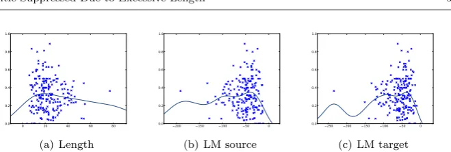
There is little reason to expect that measures of quality, such as post-editing effort, will be a linear function of the input features. To illustrate, consider how quality varies with the length of the source sentence, one of the most important feature in our arsenal. Most short inputs are easy to trans-late, and therefore we expect the translation quality to be high. In contrast medium length sentences can be much more syntactically complex, leading to much worse translations. However we do not expect that very long sentences are much worse again: in fact they may be simpler, as these sentences are often lists or other highly structured sentences which can be more easily translated. Consequently, positing a linear relationship between input length and quality is not a reasonable proposition. For this feature and many other important features, a non-linear approach is more appropriate. Fig 1 shows three exam-ples of features known to perform very well for translation quality prediction (source sentence length in 1(a), source sentence language model score in 1(b), and target sentence language model score in 1(c)) and their relationship with

post-editing distance – HTER [?], with a fittedGP_{to highlight the non}

linear-ity of the data. The same behaviour is observed with other features and other quality labels.

Like SVMs for regression – SVRs,GPs_{can describe non-linear functions}

us-ing kernels such as radial basis function (RBF). However in contrast, inference

inGP_{regression can be expressed analytically and the kernel hyper-parameters}

optimised directly using gradient descent. This avoids the need for costly grid search while also allowing the use of much richer kernel functions with many

0 20 40 60 80 0.0 0.2 0.4 0.6 0.8 1.0 (a) Length

200 150 100 50 0

0.0 0.2 0.4 0.6 0.8 1.0

(b) LM source

250 200 150 100 50 0

0.0 0.2 0.4 0.6 0.8 1.0

(c) LM target

Fig. 1 Features known to perform well for translation quality prediction (source sentence length in 1(a), source sentence language model score in 1(b), and target sentence language model score in 1(c)) and their relationship with post-editing distance – HTER, with a fitted GP to highlight the non linearity of the data.

3 2 1 0 1 2 3

2 1 0 1 2

(a) posterior samples

3 2 1 0 1 2 3

1.5 1.0 0.5 0.0 0.5 1.0 1.5

(b) fitted posterior samples

3 2 1 0 1 2 3

1.5 1.0 0.5 0.0 0.5 1.0 1.5

(c) full posterior

Fig. 2 The Bayesian posterior under a GP prior, illustrated on synthetic one-dimensional data. Figs a and b show samples from the posterior (curves) over functions given several training observations (blue dots). These differ in the values of the hyperparameters, Fig a

usesσ2

f =σ

2

n=l= 1, while Fig b has learned the MLE hyper-parameters,σ

2

f = 0.7, σ

2

n=

0.02, l= 0.3. Fig c shows the full posterior for the model in b, with the shaded blue error

denoting±one confidence interval.

are probabilistic models and can be incorporated into larger graphical models. Moreover, GPs take a fully Bayesian approach by integrating out the model parameters to support posterior inference. Unlike most other Bayesian meth-ods, GP regression supports exact posterior inference and learning (see Fig 2), without the need to resort to approximation (e.g., Markov Chain Monte Carlo sampling or variational approximations).

Formulation GP regression assumes the presence of a latent function, f :

RF → R, which maps from the input space of feature vectorsx to a scalar.

Each response value is then generated from the function evaluated at the

corresponding data point,yi=f(xi) +η, whereη ∼ N(0, σ

2

n) is added

white-noise. Formallyf is drawn from a GP prior,

f(x)∼ GP(0, k(x,x′_)),

which is parameterised by a mean (here, 0) and a covariance kernel function

k(x,x′_{). The kernel function represents the covariance (i.e., similarities in the}

response) between pairs of data points. Several draws of f from a GP prior

3 2 1 0 1 2 3 1.5

1.0 0.5 0.0 0.5 1.0 1.5

(a)l= 0.3

3 2 1 0 1 2 3

2 1 0 1 2

(b)l= 1

3 2 1 0 1 2 3

1.5 1.0 0.5 0.0 0.5 1.0 1.5

(c)l= 4

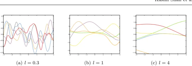
Fig. 3 Samples from a Gaussian Process prior with different length scales in an RBF kernel, showing the effect of this parameter on the smoothness of the function. We consider one

dimensional input (D= 1), setσf= 0.7 and omit the white-noise term.

Kernel (covariance) function GPs_{allow for many different kernels. Here}

we consider the RBF with automatic relevance determination,

k(x,x′_{) =σ}2

fexp −

1 2

D

X

i

(xi−x′i)

2

li

! ,

where thek(x,x′_{) is the kernel function between two data pointsx,x}′ _andD

is the number of features, andσf andli≥0 are the kernel hyper-parameters,

which control the covariance magnitude and the length scales of variation in

each dimension, respectively. This is closely related to the RBF kernel used with SVR, except that each feature is scaled independently from the others,

i.e., li =l for SVR, while GPsallow for a vector of independent values.

Fol-lowing standard practice we also include an additive white-noise term in the

kernel with variance σ2

s. The kernel hyper-parameters (σf, σn,l) are learned

from data using a maximum likelihood estimates.

The learned length scale hyper-parameters can be interpreted as encoding

the importance of a feature: the narrower the RBF (the smaller is li) the

more important a change in the feature value is to the model prediction. This is illustrated in Fig 3, which shows samples from a GP prior with different settings of the length scale: clearly the value of the input will be of less import for Fig 3(c), where the curves are mostly flat, versus Fig 3(a) which allows for rapid fluctuations. This effect can also be seen in the posterior, comparing Figs 2(a) and 2(b), where the latter’s shorter length scale allows more accurate fitting of the training points.

Feature selection A model trained usingGPs_{can be viewed as a list of features}

ranked by relevance, and this information can be used for feature selection by

discarding the lowest ranked (least useful) features.GPs_{on their own do not}

Bayesian inference Given the generative process defined above, prediction can be formulated as Bayesian inference under the posterior,

p(y_∗|x_∗,D) =

Z

f

p(y_∗|x_∗, f)p(f|D),

where x_∗ is a test input and y_∗ is its response value. The posterior p(f|D)

reflects our updated belief over possible functions after observing the training

setD, i.e.,f should pass close to the response values for each training instance

(but need not fit exactly due to additive noise). This is balanced against the biases (e.g., smoothness constraints) that arise from the GP prior. The

poste-rior is illustrated in Fig 2 (a, b), which shows several samples of f from the

posterior in (a,b), which are consistent with the observed training data, D.

The predictive posterior can be solved analytically, resulting in

y_∗∼ N kT_∗(K+σ2

nI)−

1

y, k(x∗,x∗)−k

T

∗(K+σ 2

nI)−

1

k∗

, (1)

where k_∗ = [k(x_∗,x1)k(x_∗,x2)· · ·k(x_∗,xn)]T are the kernel evaluations

be-tween the test point and the training set, and {Kij = k(xi,xj)} is the

ker-nel (gram) matrix over the training points. Note that the posterior in Eq. 1 includes not only the expected response (the mean) but also the variance, encoding the model’s uncertainty, which is important for integration into sub-sequent processing, e.g., as part of a larger probabilistic model. The posterior is illustrated in figure 2(c). Note the increasing amounts of uncertainty in the centre of the graph (wider confidence interval) where there are few nearby training instances compared to the edges where there is dense training data. This nuanced modelling of uncertainty is of great importance when combining the model into a larger probabilistic graphical model, such that uncertainty can be preserved into task based inferences.

The remaining question is how to determine the kernel hyperparameters. As stated above, these modulate the effect and strength of the GP prior, in our case determining the relative importance of each feature. The GP framework allows for kernel hyper-parameters to be learned using a maximum likelihood

estimate (type II). The marginal likelihood, p(y|X) = R

fp(y|X, f)p(f), can

be expressed analytically for GP regression (X are the training inputs), which

can be optimised with respect to the hyper-parameters for training (or model selection). Specifically, we can derive the gradient of the (log) marginal

like-lihood with respect to the model hyperparameters (i.e., σn, σf,l etc.) and

thereby find the type II maximum likelihood estimate using gradient ascent. Note that in general the marginal likelihood is non-convex in the hyperpa-rameter values, and consequently the solutions may only be locally optimal. Here we bootstrap the learning of complex models with many hyperparame-ters by initialising with the (good) solutions found for simpler models, thereby

4 Experimental settings

In our experiments, model learning is performed with an open source

imple-mentation ofGPs1_{for regression. This is used for our proposed feature selection}

method. In what follows we describe two groups of quality estimation datasets: the first group contains various datasets for which we have extracted common

feature sets using the QuEst framework [?,?] (Section 4.1); the second group

contains a single dataset with various feature sets provided as part of the WMT12 quality estimation shared task (Section 4.2).

4.1 Datasets with QuEst features

The following datasets have a common feature set and are available for

down-load.2

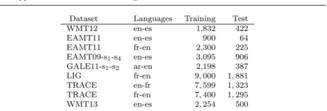
The statistics of these datasets are shown in Table 1.

WMT12 English-Spanish news sentence translations produced by a

phrase-based (PB) Moses “baseline” SMT system,3

and judged for post-editing effort in 1-5 (highest-lowest), taking a weighted average of three annotators.

EAMT11 English-Spanish en-es) and French-English

(EAMT11-fr-en) news sentence translations produced by a PB-SMT Moses baseline sys-tem and judged for post-editing effort in 1-4 (highest-lowest).

EAMT09 English sentences from the European Parliament corpus translated

by four SMT systems (two Moses-like PB-SMT systems and two fully discrim-inative training systems) into Spanish and scored for post-editing effort in 1-4

(highest-lowest). Systems are denoted by s1-s4.

GALE11 Arabic newswire sentences translated by two Moses-like PB-SMT

systems into English and scored for adequacy in 1-4 (worst-best). Systems are

denoted by s1-s2.

TRACE English-French (en-fr) and French-English (fr-en) sentence

transla-tions produced by two MT systems: a rule-based system (Reverso) and LMSI’s

statistical MT system [?]. English-French contains a mixture of data from

Ted Talks, WMT news, SemEval-2 Cross-Lingual Word Sense Disambigua-tion, and translation requests from Softissimo’s online translation portal (the Reverso system), which can be thought of as user-generated content. The French-English data contains sentences from the OWNI – a free French online newspaper, Ted Talks and translation requests from Softissimo’s online trans-lation portal. All transtrans-lations have been post-edited and the HTER scores are

1

http://sheffieldml.github.io/GPy/

2

http://www.dcs.shef.ac.uk/~lucia/resources.html 3

Dataset Languages Training Test

WMT12 en-es 1,832 422

EAMT11 en-es 900 64

EAMT11 fr-en 2,300 225

EAMT09-s1-s4 en-es 3,095 906

GALE11-s1-s2 ar-en 2,198 387

LIG fr-en 9,000 1,881

TRACE en-fr 7,599 1,323

TRACE fr-en 7,400 1,295

WMT13 en-es 2,254 500

Table 1 Number of sentences in our datasets. Figures for EAMT09-s1-s4and GALE11-s1

-s2indicate number of sentences per MT system.

used as quality labels. For each language pair, 1,000 translations have been

post-edited by two translators independently. We simply concatenated these in our datasets.

LIG French-English sentence translations of various editions of WMT news

test sets, produced by a customised version of a PB-SMT Moses system by the

LIG group [?]. These sentences have been post-edited by a human translator,

and labelled for HTER.

WMT13 English-Spanish sentence translations of news texts produced by a

PB-SMT Moses baseline system. These were then post-edited by a professional translator and labelled for post-editing effort using HTER. This is a superset of the WMT12 dataset, with 500 additional sentences for test, and a different quality label.

4.1.1 Feature sets

The features for these datasets are extracted using the open source toolkit

QuEst.4

We differentiate betweenblack-box(BB) andglass-box(GB) features,

as only BB are available for all datasets (we did not have access to all MT systems that produced the other datasets). For the WMT12 and GALE11 datasets, we experimented with both BB and GB features. The BB feature sets are the same for all datasets, except for the Arabic-English datasets, where language-specific features supplement the initial set of features, and for the WMT13 dataset, where advanced features dependent on external resources like parsers have been exploited.

We also distinguish one special feature: thepseudo-reference(PR), as this

is not a standard feature in that it requires another MT system to be extracted. This feature consists in translating the source sentence using another MT

sys-tem (in our case, Google Translate) to obtain apseudo-reference. The

geomet-ric mean of (lambda-smoothed) 1-to-4-gram precision scores (i.e. a smoothed

4

version of BLEU to avoid 0-counts without the brevity penalty) is then com-puted between the original MT and this pseudo-reference. We note that the better the external MT system, the closer the pseudo-reference translation is to a human translation, and therefore the more reliable this feature becomes.

For each dataset we built four QE systems, each with a feature set:

– BL: 17 features that performed well across languages in previous work and

were used as baseline in the WMT12-13 QE shared tasks.

– number of tokens in the source & target sentences

– average source token length

– average number of occurrences of the target word within the target

sentence

– number of punctuation marks in source and target sentences

– language model (LM) probability of source and target sentences using

3-gram LMs built from the source/target sides of SMT training corpus

– average number of translations per source word as given by IBM 1

model thresholded such thatP(t|s)>0.2

– same as above withP(t|s)>0.01 weighted by the inverse frequency of

each word in the source side of the SMT training corpus

– percentage of unigrams, bigrams and trigrams in frequency quartiles 1

(lower frequency words) and 4 (higher frequency words) in the source side of the SMT training corpus

– percentage of unigrams in the source sentence seen in the source side

of the SMT training corpus

– AF: All features available for the dataset. This is a superset of the above,

where:

– For the experiments with BB features we have a common set of 80

features for all datasets, and additional 43 language specific features for the Arabic-English datasets, or additional advanced features for the WMT13 dataset, for which resources had been previously curated.

– For the experiments with GB features we have all MT system-dependent

features (varying according to the actual type of MT system) available

for the GALE11-s1(39), GALE11-s2 (48), and WMT12 (47) datasets.

For a comprehensive list, we refer the reader to the QuEst project website.4

– BL+PR: 17 baseline features along with a pseudo reference feature.

– AF+PR: All features available (BB, GB or BB+GB) plus the

pseudo-reference feature.

4.2 WMT12 datasets

This is exactly the same as the WMT12 dataset described above. However, as feature sets, we use those provided by all but one of the participating teams

in the WMT12 shared task on QE.5

These very diverse feature sets, with

5

These feature sets were made available by the task organisers athttp://www.dcs.shef.

features of many different natures, although some overlap with the QuEst

features exists in most cases. We denote each of these feature setAF. We note

however that in a few cases these are only a subset of the features actually used

in the shared task, e.g.UU, since the participants could not provide us with

the full feature sets. This explains the difference between the official scores

reported in [?] and our figures. This difference can also be explained by the

learning algorithms: while we used GPs_{, participants have used SVRs, M5P}

and other algorithms. Some of these feature sets already result from feature selection techniques.

SDL [?]: 15 features selected after an exhaustive search algorithm based on all

possible combinations of features. This is the optimal set used by the winning submission. It includes many of the baseline features, the pseudo-reference feature, phrase table probabilities, and a few part-of-speech tag alignment features.

UU [?]: 82 features, a subset of those used in the shared-task as the parse tree

features (based on tree-kernels) were not provided by the participants. These are similar to the common BL and BB features presented above and include various source and target LM features, average number of translations per source word, number of tokens matching certain patterns (hyphens, ellipsis, etc.), percentage of n-grams seen in corpus, percentage of non-aligned words, etc.

UEdin [?]: 56 black-box features including source translatability, named enti-ties, LM back-off features, discriminative word-lexicon, edit distance between source sentence and the SMT source training corpus, and word-level features based on neural networks to select a subset of relevant words among all words in the corpus.

Loria [?]: 49 features including 1-5gram LM and back-off LM features, inter-lingual and cross-inter-lingual mutual information features, IBM1 model average translation probability, punctuation checks, and out-of-vocabulary rate.

TCD [?]: 43 features based on the similarity between the (source or target)

sentence and a reference set (the SMT training corpus or Google N-grams) with n-grams of different lengths, including the TF-IDF metric.

WLV-SHEF [?]: 147 features which are a superset of the common 80

UPC [?]: 56 features on top of the baseline features. Most of these features are based on different language models estimated on reference and automatic Spanish translations.

4.3 Feature selection techniques

As previously described, our proposed technique for feature selection usesGPs_.

In each dataset, features are first normalised. Each feature is centred and scaled to have zero mean and unit standard deviation. For feature ranking,

the models are trained on the full training sets, except in the FS(GP-dev)

setting (below). The RBF widths, scale and noise variance are initialised with

an isotropic kernel (with a single length scale, li = l) which helps to avoid

local minima. We apply a sparse approximation method for inference, known as FITC (Fully Independent Training Conditional), which bases parameter learning on a few inducing points in the training set instead of the entire training set. This approximation technique is used to make the learning less computationally expensive and therefore faster, which is important for large training sets. The hyper-parameters are learned using gradient descent with a maximum of 100 iterations and cross-validation on the training set. A forward selection approach is then used to select features ranked from top to worst and

train models using GPs_{with increasing numbers of features and all available}

training data.

Four variant of selection techniques were used in our experiments, all

ap-plied on the entire set of features (AF+PRfor the QuEst datasets, andAF

for the WMT12 datasets):

– FS(GP-dev): Feature selection onAF+PR for automatic ranking and

selection of top features withGPs_{on a development set and applied to test}

set.

– FS(GP-fixed): Feature selection onAF+PRfor automatic ranking and

selection of top features withGPs_{and a fixed number of features (threshold}

pre-– FS(GP-test): Feature selection on AF+PR for automatic ranking and

selection of top features with GPs_{directly on test set (oracle selection).}

– FS(RL): Feature selection with Randomized Lasso.

InFS(GP-dev), a development set is randomly selected from the training

data for each of the dataset. In each of the datasets, we extracted the same number of sentences for development as there were for the test set. The de-velopment set was then used to choose the cutoff point in the ranked set of

features generated by theGP_{model, i.e., where to stop selecting features. Once}

we performed feature selection over development set, the full training set was used to train the final models.

FS(GP-fixed)is based on pre-defined threshold on number of features to

experiments, we selected 17 as fixed threshold for two reasons: it falls within this range and it allows for an interesting comparison with the intuitively selected 17 baseline features.

In FS(GP-test), the selected set is evaluated under an oracle condition,

where the optimal number of features is decided based on the best perfor-mance obtained directly on the test set. This experiment aimed to study the

upper bound in performance of the GPs_{-based method for feature selection.}

The subset of top ranked features that minimises error in each test set is selected.

As an alternative approach to GPs_{, we use Randomized Lasso, FS(RL),}

for feature selection. Randomised Lasso repeatedly resamples the training data and fits a Lasso regression model on each sample. A feature is selected for the final model if it is selected (i.e., assigned a non-zero weight) in at least 25% of the samples (we do this 1000 times). This strategy improves the robustness of Lasso in the presence of high dimensional and correlated inputs. It should

be noted that FS(RL) automatically selects the number of features to be

used for training. The final models are still trained usingGPs_{on the selected}

features.

4.4 Evaluation metrics

To evaluate the prediction models we use Mean Absolute Error (MAE), its squared version – Root Mean Squared Error (RMSE), plus the Relative Ab-solute Error (RAE) and its squared version – Relative Squared Error (RSE). MAE is used as the main metric on the charts for a comparative analysis. RAE provides the average error relative to a simple predictor, which is just the average of the true values. It is meant to provide some form of comparison across prediction models for different datasets.

MAE =

PN

i=1|H(si)−V(si)|

N RMSE =

s PN

i=1(H(si)−V(si)) 2

N

RAE =

n

X

i=1

|H(si)−V(si)|

n

X

i=1

|V¯(s)−V(si)|

RSE =

v u u u u u u u t

n

X

i=1

(H(si)−V(si))

2

n

X

i=1

( ¯V(s)−V(si))

2

where:

N =|S|is the number of test instances,

H(si) is the predicted score forsi,

V(si) is the true (human) score forsi,

¯

5 Results

We note that preliminary results for some of the datasets used here have been

reported in [?]. The following results include additional datasets and further

analysis.

5.1 Results on QuEst feature sets

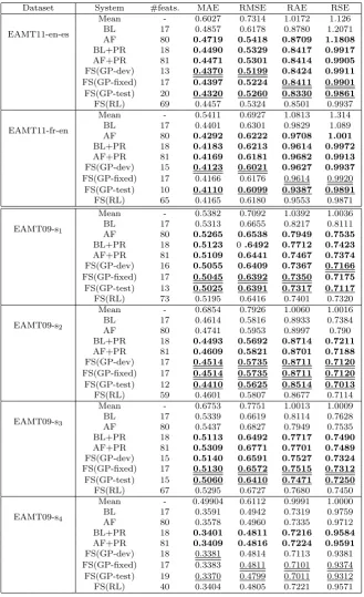
The error scores for all datasets with common (QuEst) black-box (BB) features are reported in Tables 2 and 3, while Table 4 shows the results with glass-box (GB) features for a subset of these datasets, and Table 5 the results with BB and GB features together for the latter datasets. For each Table and dataset, bold-faced figures represent results that are significantly better (paired t-test

with p≤ 0.05) with respect to the following comparisons – where available,

while underlined figures represent best results overall and double underlined figures, the second best results:

– BL vs AF;

– BL vs BL+PR;

– AF vs AF+PR; and

– Each feature selection techniques versus AF+PR.

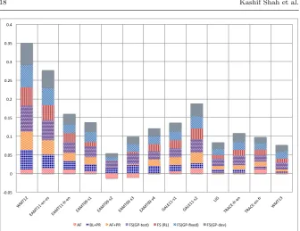
In what follows we take a closer look at some of these comparisons, as well as the difference between different types of feature selection methods. We summarise these comparisons graphically in Fig 4. This figure shows the improvements of different feature sets over the BL results. We also discuss the impact of using GB features against BB features only, showing the im-provements of various feature sets over the use of black-box features in Fig 6.

Baseline features vs all feature sets Adding more features (systemsAF)

leads to better results in most cases as compared to the baseline systemsBL,

except for some of the EAMT-09 datasets. However, these are small and in some cases not significant improvements. Adding more features may bring more relevant information, but at the same time it makes the representation more sparse and the learning prone to overfitting. Larger improvements over the baseline come from using either a pseudo-reference feature or performing feature selection, as we discuss in what follows.

Impact of the pseudo-reference feature Adding a single feature, the

pseudo-reference (systems BL+PR) to our baseline improves results in all

datasets, often by a large margin. Similar improvements are observed by adding

Dataset System #feats. MAE RMSE RAE RSE

EAMT11-en-es

Mean - 0.6027 0.7314 1.0172 1.126

BL 17 0.4857 0.6178 0.8780 1.2071

AF 80 0.4719 0.5418 0.8709 1.1808

BL+PR 18 0.4490 0.5329 0.8417 0.9917

AF+PR 81 0.4471 0.5301 0.8414 0.9905

FS(GP-dev) 13 0.4370 0.5199 0.8424 0.9911

FS(GP-fixed) 17 0.4397 0.5224 0.8411 0.9901

FS(GP-test) 20 0.4320 0.5260 0.8330 0.9861

FS(RL) 69 0.4457 0.5324 0.8501 0.9937

EAMT11-fr-en

Mean - 0.5411 0.6927 1.0813 1.314

BL 17 0.4401 0.6301 0.9829 1.089

AF 80 0.4292 0.6222 0.9708 1.001

BL+PR 18 0.4183 0.6213 0.9614 0.9972

AF+PR 81 0.4169 0.6181 0.9682 0.9913

FS(GP-dev) 15 0.4123 0.6021 0.9627 0.9937

FS(GP-fixed) 17 0.4166 0.6176 0.9614 0.9920

FS(GP-test) 10 0.4110 0.6099 0.9387 0.9891

FS(RL) 65 0.4165 0.6180 0.9553 0.9871

EAMT09-s1

Mean - 0.5382 0.7092 1.0392 1.0036

BL 17 0.5313 0.6655 0.8217 0.8111

AF 80 0.5265 0.6538 0.7949 0.7535

BL+PR 18 0.5123 0.6492 0.7712 0.7423

AF+PR 81 0.5109 0.6441 0.7467 0.7374

FS(GP-dev) 16 0.5055 0.6409 0.7367 0.7166

FS(GP-fixed) 17 0.5045 0.6392 0.7350 0.7175

FS(GP-test) 13 0.5025 0.6391 0.7317 0.7117

FS(RL) 73 0.5195 0.6416 0.7401 0.7320

EAMT09-s2

Mean - 0.6854 0.7926 1.0060 1.0016

BL 17 0.4614 0.5816 0.8933 0.7384

AF 80 0.4741 0.5953 0.8997 0.790

BL+PR 18 0.4493 0.5692 0.8714 0.7211

AF+PR 81 0.4609 0.5821 0.8701 0.7188

FS(GP-dev) 17 0.4514 0.5735 0.8711 0.7120

FS(GP-fixed) 17 0.4514 0.5735 0.8711 0.7120

FS(GP-test) 12 0.4410 0.5625 0.8514 0.7013

FS(RL) 59 0.4601 0.5807 0.8677 0.7114

EAMT09-s3

Mean - 0.6753 0.7751 1.0013 1.0009

BL 17 0.5339 0.6619 0.8114 0.7628

AF 80 0.5437 0.6827 0.7949 0.7535

BL+PR 18 0.5113 0.6492 0.7717 0.7490

AF+PR 81 0.5309 0.6771 0.7701 0.7489

FS(GP-dev) 15 0.5140 0.6591 0.7527 0.7324

FS(GP-fixed) 17 0.5130 0.6572 0.7515 0.7312

FS(GP-test) 15 0.5060 0.6410 0.7471 0.7250

FS(RL) 67 0.5295 0.6727 0.7680 0.7450

EAMT09-s4

Mean - 0.49904 0.6112 0.9991 1.0000

BL 17 0.3591 0.4942 0.7319 0.9759

AF 80 0.3578 0.4960 0.7335 0.9712

BL+PR 18 0.3401 0.4811 0.7216 0.9584

AF+PR 81 0.3409 0.4816 0.7224 0.9591

FS(GP-dev) 18 0.3381 0.4814 0.7113 0.9381

FS(GP-fixed) 17 0.3383 0.4811 0.7101 0.9374

FS(GP-test) 19 0.3370 0.4799 0.7011 0.9312

FS(RL) 40 0.3404 0.4805 0.7221 0.9571

Dataset System #feats. MAE RMSE RAE RSE

WMT12

Mean - 0.8278 0.9898 1.0247 1.0263

BL 17 0.6821 0.8117 0.8622 0.7152

AF 80 0.6717 0.8103 0.8476 0.6954

BL+PR 18 0.6290 0.7729 0.8139 0.6678

AF+PR 81 0.6324 0.7735 0.7745 0.6699

FS(GP-dev) 15 0.6231 0.7658 0.7719 0.6651

FS(GP-fixed) 17 0.6224 0.7645 0.7701 0.6644

FS(GP-test) 19 0.6131 0.7598 0.7613 0.6586

FS(RL) 71 0.6335 0.7724 0.7755 0.6709

WMT13

Mean - 0.1438 0.1792 1.0036 1.0009

BL 17 0.1411 0.1812 0.9723 1.086

AF 114 0.1389 0.1775 0.9211 0.9713

BL +PR 18 0.1409 0.1802 0.9711 1.063

AF+PR 115 0.1367 0.1759 0.9181 0.9693

FS(GP-dev) 19 0.1217 0.1411 0.8907 0.9577

FS(GP-fixed) 17 0.1242 0.1489 0.8911 0.9581

FS(GP-test) 19 0.1207 0.1481 0.8844 0.9531

FS(RL) 101 0.1317 0.1691 0.9201 0.9709

GALE11-s1

Mean - 0.5823 0.7214 0.8533 0.8125

BL 17 0.5462 0.6885 0.8186 0.7715

AF 123 0.5399 0.6805 0.8017 0.7619

BL+PR 18 0.5301 0.6814 0.7929 0.7595

AF+PR 81 0.5249 0.6766 0.7905 0.7520

FS(GP-dev) 21 0.5220 0.6751 0.7871 0.7581

FS(GP-fixed) 17 0.5231 0.6761 0.7856 0.7577

FS(GP-test) 27 0.5210 0.6701 0.7811 0.7434

FS(RL) 56 0.5258 0.6749 0.7914 0.7530

GALE11-s2

Mean - 0.5850 0.7527 0.8573 0.8313

BL 17 0.5540 0.7117 0.8287 0.7978

AF 123 0.5401 0.6911 0.8232 0.7931

BL+PR 18 0.5401 0.7014 0.8221 0.7901

AF+PR 81 0.5249 0.6806 0.8154 0.7892

FS(GP-dev) 22 0.5197 0.6769 0.8133 0.7853

FS(GP-fixed) 17 0.5219 0.6794 0.8123 0.7841

FS(GP-test) 31 0.5194 0.6779 0.8081 0.7815

FS(RL) 54 0.5239 0.6805 0.8134 0.7899

LIG

Mean - 0.1326 0.1727 .9938 1.0245

BL 17 0.1250 0.1638 0.9369 0.9223

AF 80 0.1227 0.1631 0.9344 0.9209

BL+PR 18 0.1159 0.1527 0.9312 0.9191

AF+PR 81 0.1161 0.1534 0.9313 0.9183

FS(GP-fixed) 17 0.1087 0.1504 0.9287 0.9135

FS(GP-dev) 13 0.1077 0.1493 0.9284 0.9145

FS(GP-test) 13 0.1054 0.1489 0.9227 0.9099

FS(RL) 69 0.1154 0.1519 0.9321 0.9178

TRACE-fr-en

Mean - 0.1868 0.2470 1.0079 1.0030

BL 17 0.1807 0.2429 0.9749 0.9695

AF 80 0.1776 0.2422 0.9678 0.9611

BL+PR 18 0.1729 0.2210 0.9611 0.9554

AF+PR 81 0.1687 0.2127 0.9601 0.9521

FS(GP-dev) 18 0.1564 0.2081 0.9571 0.9499

FS(GP-fixed) 17 0.1597 0.2101 0.9565 0.9487

FS(GP-test) 19 0.1554 0.2089 0.9515 0.9421

FS(RL) 72 0.1654 0.2109 0.9589 0.9501

TRACE-en-fr

Mean - 0.1891 0.2460 1.0004 1.0021

BL 17 0.1782 0.2389 0.9315 0.9354

AF 80 0.1657 0.2279 0.9261 0.9292

BL+PR 18 0.1729 0.2210 0.9292 0.9314

AF+PR 82 0.1637 0.2127 0.9211 0.9226

FS(GP-dev) 15 0.1615 0.2133 0.9209 0.9221

FS(GP-fixed) 17 0.1612 0.2127 0.9201 0.9211

FS(GP-test) 18 0.1611 0.2131 0.9178 0.9193

FS(RL) 71 0.1633 0.2241 0.9209 0.9220

Dataset System #features MAE RMSE RAE RSE

WMT12 AF 47 0.7066 0.8445 0.9114 0.7467

FS(GP-dev) 19 0.6789 0.8318 0.8931 0.7210

FS(GP-fixed) 17 0.6775 0.8314 0.8914 0.7196

FS(GP-test) 21 0.6755 0.8298 0.8814 0.7119

FS(RL) 35 0.6921 0.8388 0.9057 0.7411

GALE11-s1 AF 39 0.5736 0.7402 0.8516 0.8131

FS(GP-dev) 18 0.5715 0.7385 0.8499 0.8080

FS(GP-fixed) 17 0.5732 0.7381 0.8491 0.8098

FS(GP-test) 19 0.5702 0.7361 0.8441 0.8060

FS(RL) 33 0.5781 0.7481 0.8501 0.8111

GALE11-s2

AF 48 0.5540 0.6979 0.8317 0.8060

FS(GP-dev) 21 0.5451 0.6998 0.8243 0.8005

FS(GP-fixed) 13 0.5491 0.6944 0.8261 0.8011

FS(GP-test) 13 0.5411 0.6934 0.8220 0.8001

FS(RL) 41 0.5512 0.6950 0.8301 0.8041

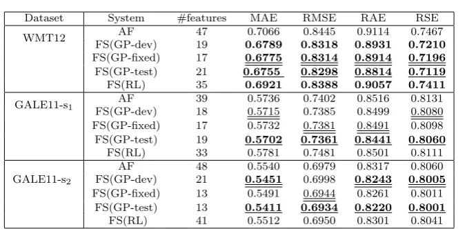
Table 4 Results with GB features.

Dataset System #features MAE RMSE RAE RSE

WMT12 AF 128 0.7185 0.8451 0.9137 0.7507

FS(GP-dev) 25 0.6121 0.7582 0.7692 0.6629

FS(GP-fixed) 17 0.6161 0.7591 0.7703 0.6639

FS(GP-test) 29 0.6101 0.7561 0.7679 0.6611

FS(RL) 99 0.6601 0.8098 0.7815 0.6779

GALE11-s1 AF 163 0.5455 0.6722 0.8226 0.7755

FS(GP-dev) 27 0.5162 0.6699 0.7801 0.7411

FS(GP-fixed) 17 0.5170 0.6701 0.7810 0.7421

FS(GP-test) 30 0.5150 0.6681 0.7785 0.7384

FS(RL) 132 0.5310 0.6731 0.7911 0.7501

GALE11-s2

AF 172 0.5239 0.6529 0.8177 0.7915

FS(GP-dev) 27 0.5120 0.6441 0.8094 0.7812

FS(GP-fixed) 17 0.5119 0.6451 0.8111 0.7823

FS(GP-test) 17 0.5109 0.6431 0.8063 0.7795

FS(RL) 132 0.5155 0.6499 0.8144 0.7887

Table 5 Results with common BB & GB features.

Impact of feature selection Our experiments with feature selection using

bothGPs_andRL_{led to significant improvements over the entire set of features.}

Feature selection withGPs_{has shown better performance over feature selection}

withRL_.

For a more comprehensive overview of the results of feature selection using

GPs_{, we plot the MAE error scores (on the test sets) for different cut-off points}

on the features in our forward selection method after features are ranked by

GPs_{. The plots for two of our datasets are given in Fig 5. Theyaxis shows the}

MAE scores, while thexaxis shows the number of features selected. Generally,

!∀#∀∃% ∀% ∀#∀∃% ∀#&% ∀#&∃% ∀#∋% ∀#∋∃% ∀#(% ∀#(∃% ∀#)%

∗+, &∋%

−.+, &&!/

0!/1 %

−.+, &&!2

3!/0 %

−.+, ∀4!1

&%

−.+, ∀4!1

∋%

−.+, ∀4!1

(%

−.+, ∀4!1

)%

5.6 −&&!

1&%

5.6 −&&!

1∋% 675%

,8. 9−!2

3!/0 %

,8. 9−!/

0!23 %

∗+, &(%

.:% ;6<=8% .:<=8% :>?5=!≅/1≅Α% :>%?86Α% :>?5=!ΒΧ/DΑ% :>?5=!D/ΕΑ%

Fig. 4 Improvements of various feature-sets over the BL features. The height of the bar representing a feature set is proportional to the actual improvement it brings over the results with the baseline feature set.

while a very small number of features is naturally insufficient, adding features

ranked lower byGPs_{degrades performance. Similar curves were observed for}

all datasets with slightly different ranges for optimal numbers of features and best score. It is interesting to note that the best performance on most datasets

is observed using 10-20 top-ranked features. This explains whyFS(GP-fixed)

performs as well asFS(GP-dev)or evenFS(GP-test), in most cases. Given

thatFS(GP-dev)andFS(GP-fixed)perform equally well in most cases, the

choice between them could be guided by the size of the dataset: if enough data is available to put a development set aside, this should be preferable, while

FS(GP-fixed)should be used as a cheaper alternative approach if necessary.

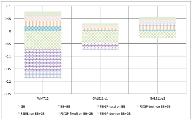
Black-box versus glass-box features GB features on their own perform

worse than BB features (Fig 6), but in all three datasets the combination of GB and BB followed by feature selection resulted in significantly lower error than using only BB features with feature selection, showing that the two features sets are complementary.

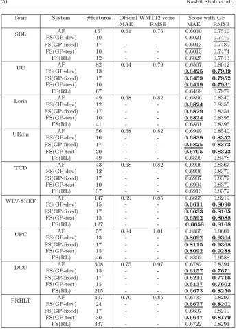
5.2 Results on WMT12 datasets

0 10 20 30 40 50 60 70 80 0.43

0.435 0.44 0.445 0.45 0.455 0.46

Number of features

M

A

E

0 10 20 30 40 50 60 70 80 0.61

0.62 0.63 0.64 0.65 0.66 0.67

Numer of features

M

A

E

Fig. 5 Error on (a) WMT12 and (b) EAMT11-en-es datasets with all BB features ranked

byGPs.

!∀#∃%& !∀#∃& !∀#∋%& !∀#∋& !∀#∀%& ∀& ∀#∀%& ∀#∋&

()∗∋∃& +,−.∋∋!/∋& +,−.∋∋!/∃&

+0& 001+0& 234+5!67/68&9:&00& 234+5!67/68&9:&001+0&

234;−8&9:&001+0&&&&& 234+5!<=7>8&9:&001+0&&&&& 234+5!>7?8&9:&001+0&&&&&

Fig. 6 Improvements of various feature sets over black-box features (AF+PR).

participating in the WMT12 QE shared task. These feature sets are very di-verse in terms of the types of features, resources used, and their sizes. As

shown in Table 6, we observed similar results: feature selection withGPs_has

the potential to outperform models with all initial feature sets. For these

ex-periments, the significance is checked between system AF trained with GPs

versus each feature selection techniques. Improvements were observed even on feature sets which had already been produced as a result of some other fea-ture selection technique. Table 6 also shows the official results from the shared

task [?], which are often different from the results obtained withGPs_even

be-fore feature selection, simply because of differences in the learning algorithms

used. In some cases results withGPs_{before feature selection are better, notably}

for WLV-SHEF – which uses a large set of linguistically-motivated features,

Team System #features Official WMT12 score Score with GP

MAE RMSE MAE RMSE

SDL AF 15∗ 0.61 0.75 0.6030 0.7510

FS(GP-dev) 10 - - 0.6021 0.7479

FS(GP-fixed) 17 - - 0.6013 0.7489

FS(GP-test) 10 - - 0.6013 0.7474

FS(RL) 12 - - 0.6025 0.7513

UU AF 82 0.64 0.79 0.6507 0.8012

FS(GP-dev) 13 0.6425 0.7939

FS(GP-fixed) 17 0.6459 0.7952

FS(GP-test) 10 0.6419 0.7931

FS(RL) 67 0.6489 0.7979

Loria AF 49 0.68 0.82 0.6866 0.8340

FS(GP-dev) 12 - - 0.6824 0.8355

FS(GP-fixed) 17 - - 0.6829 0.8351

FS(GP-test) 10 - - 0.6824 0.8395

FS(RL) 41 - - 0.6861 0.8395

UEdin AF 56 0.68 0.82 0.6949 0.8540

FS(GP-dev) 16 - - 0.6839 08352

FS(GP-fixed) 17 - - 0.6825 08373

FS(GP-test) 20 - - 0.6795 0.8323

FS(RL) 49 - - 0.6899 0.8478

TCD AF 43 0.68 0.82 0.6906 0.8367

FS(GP-dev) 12 - - 0.6906 0.8370

FS(GP-fixed) 17 - - 0.6907 0.8372

FS(GP-test) 10 - - 0.6904 0.8370

FS(RL) 37 - - 0.6913 0.8372

WLV-SHEF AF 147 0.69 0.85 0.6665 0.8219

FS(GP-dev) 15 - - 0.6611 0.8090

FS(GP-fixed) 17 - - 0.6633 0.8105

FS(GP-test) 15 - - 0.6592 0.8088

FS(RL) 127 - - 0.6658 0.8168

UPC AF 57 0.84 1.01 0.8365 0.9601

FS(GP-dev) 13 - - 0.8092 0.9304

FS(GP-fixed) 17 - - 0.8115 0.9368

FS(GP-test) 15 - - 0.8092 0.9288

FS(RL) 46 - - 0.8302 0.9588

DCU AF 308 0.75 0.97 0.6782 0.8394

FS(GP-dev) 15 - - 0.6157 0.7671

FS(GP-fixed) 17 - - 0.6211 0.7716

FS(GP-test) 15 - - 0.6137 0.7602

FS(RL) 215 - - 0.6673 0.8250

PRHLT AF 497 0.70 0.85 0.6733 0.8297

FS(GP-dev) 24 - - 0.6677 0.8201

FS(GP-fixed) 17 - - 0.6697 0.8219

FS(GP-test) 30 - - 0.6647 0.8179

FS(RL) 337 - - 0.6722 0.8291

Table 6 Results on WMT12 feature sets. * indicates that the initial feature sets already resulted from feature selection.

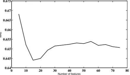
example, Fig 7 shows the Uppsala University feature set, with the lowest error score for the 15 top-ranked features.

0 10 20 30 40 50 60 70 80 0.64

0.645 0.65 0.655 0.66 0.665 0.67 0.675

Number of features

MAE

Fig. 7 Error on 82 UU dataset with all features ranked byGPs.

5.3 Commonly selected features

Next we investigate whether it is possible to identify a common subset of features which are selected for the optimal feature sets in most datasets. To do that, we took the average rank of each feature across all datasets containing common feature sets. The 10 top and bottom ranked features, along with their average rankings, are shown in Table 7.

Interestingly, not all top ranked features are among the 17 reportedly good baseline features. All of these features are language-independent. Also, most of them are simple and straightforward to extract: they either do not rely on external resources, or use resources that are easily available, such as tools for LM (e.g., SRILM), or word-alignment (e.g., GIZA++).

The same analysis on the feature sets from the WMT12 shared task is not possible, given the very little overlap in features used by the different feature sets.

6 Conclusions and future work

Top-ranked feature Avg. rank

source sentence perplexity 9.12

number of mismatched quotation marks 11.28

source sentence perplexity without end of sentence marker 12.57

number of tokens in target 15.59

number of tokens in source 15.61

average number of translations per

source word in the sentence (threshold in giza: prob>0.1) 16.42

LM log probability of POS of the target 18.33

average number of translations per source word in the sentence

(threshold in giza: prob > 0.2) weighted by the inverse frequency

of each word in the source corpus

19.12

pseudo-reference 19.99

absolute difference between no tokens in source and target normalised by source length

20.45

Bottom-ranked features Avg. rank

absolute difference between number of commas in source and target 73.10

percentage of distinct unigrams seen in the corpus (in all quartiles) 69.13

average unigram frequency in quartile 3 of frequency (lower frequency words) in the corpus of the source sentence

65.14

absolute difference between number of : in source and target nor-malised by target length

64.19

absolute difference between number of : in source and target 62.12

percentage of tokens in the target which do not contain only a-z 61.16

number source tokens that do not contain only a-z 61.01

average number of translations per source word in the sentence

(threshold in giza: prob>0.5)

59.66

percentage of punctuation marks in target 59.11

percentage of content words in the target 58.83

Table 7 Top and bottom ranked features based on their averageGPrank across datasets.

an empirically pre-defined set of features (17). The proposed feature selection technique has also been shown to improve the performance of all participat-ing systems in the WMT12 shared task on quality estimation. Finally, our analysis led to the identification of a set of features which perform well on av-erage across many datasets with different language pairs, machine translation systems, text domains and quality labels.

Acknowledgments