33% Classification Accuracy Improvement in a Motor Imagery Brain Computer Interface

(1)

http://www.scirp.org/journal/jbise J. Biomedical Science and Engineering, _{2017, Vol. 10, (No. 6), pp: 326-341}

https://doi.org/10.4236/jbise.2017.106025 326 J. Biomedical Science and Engineering

33% Classification Accuracy Improvement in a Motor

Imagery Brain Computer Interface

E. Bou Assi1, S. Rihana2, M. Sawan1

1_{Polystim Neurotech Lab, Institute of Biomedical Engineering, Polytechnique Montreal, QC, Canada;}2_Biomedical Engineering Department, Holy Spirit University of Kaslik, Jounieh, Lebanon

Correspondence to: E. Bou Assi, [email protected]

Keywords: Brain Computer Interface, Motor Imagery, Signal Processing, Feature Extraction, Kmeans Clustering, Classification

This work is licensed under the Creative Commons Attribution International License (CC BY 4.0). http://creativecommons.org/licenses/by/4.0/

ABSTRACT

A right-hand motor imagery based brain-computer interface is proposed in this work. Such a system requires the identification of different brain states and their classification. Brain signals recorded by electroencephalography are naturally contaminated by various noises and interferences. Ocular artifact removal is performed by implementing an automatic me-thod “Kmeans-ICA” which does not require a reference channel. This meme-thod starts by de-composing EEG signals into Independent Components; artefactual ones are then identified using Kmeans clustering, a non-supervised machine learning technique. After signal pre-processing, a Brain computer interface system is implemented; physiologically interpretable features extracting the wavelet-coherence, the wavelet-phase locking value and band power are computed and introduced into a statistical test to check for a significant difference be-tween relaxed and motor imagery states. Features which pass the test are conserved and used for classification. Leave One Out Cross Validation is performed to evaluate the per-formance of the classifier. Two types of classifiers are compared: a Linear Discriminant Analysis and a Support Vector Machine. Using a Linear Discriminant Analysis, classifica-tion accuracy improved from 66% to 88.10% after ocular artifacts removal using Kmeans-ICA. The proposed methodology outperformed state of art feature extraction me-thods, namely, the mu rhythm band power.

1. INTRODUCTION

The first Brain-Computer Interface (BCI) based system was proposed by Vidal in 1973 hundred years after the discovery of brain electrical activity [1]. Motor imagery based BCI is of particular importance

(2)

since it is a purely cognitive method that does not require an external stimulus or excitation such as in P300 or Evoked Electroencephalography (EEG) potential based BCIs. Such a system translates human thoughts into commands bypassing the peripheral nervous system. In an attempt to control a BCI, the user may modulate brain activity patterns. These should be automatically identified by the BCI classification algorithm and translated into commands. Although much effort has been put towards a better perfor-mance of BCI systems, the ability to accurately identify different motor imagery states remains elusive [2]. EEG is considered as the gold standard to capture electrical brain currents [3] flowing during synaptic ex-citations of pyramidal neurons in the cerebral cortex [4]. In this work, non-invasive EEG is used for re-cording brain’s electrical activity by placing electrodes along the scalp. Therefore, signals are contaminated by external and internal inferences and need to be processed before analysis and feature extraction. These noises could be ocular artifacts, Electrocardiogram (ECG), Electromyogram (EMG) and many others. Ocular artifacts, mainly eye blinking, mostly affect the performance of an EEG based BCI system since they overlap with the EEG frequency of interest [5]. While other artifacts such as EMG can be minimized by asking the subject to be relaxed during the acquisition, it is impossible for almost all people to control their eye blinking. Additionally, it has been recently shown that asking the subjects to avoid blinking can induce an additive cognitive task introducing a bias in certain experiments [6]. Two main strategies have been proposed to attenuate this overlapping artifact. The first consists of a visual identification and rejec-tion of epochs contaminated by ocular artifacts. This method is not accurate since it is subjective (related to the observer) and is usually accompanied by a loss of data [7]. The second strategy relies on conven-tional Electrooculogram (EOG) correction methods such as regression [8], linear filtering [9], Principal Components Analysis (PCA) [10] and Independent Component Analysis (ICA). ICA has shown to be very effective for ocular artifacts filtering with results favorable to those obtained with PCA or regression based methods [6]. However, this blind source separation (BSS) based technique requires the identification of artefactual components. Many researches have been conducted in this field; the traditional approach is a manual identification of artefactual Independent Components (ICs) by interpreting activation time series, scalp topographies, and frequency distribution. Although this approach may show usable for offline EEG preprocessing and analysis, it is not suitable for online BCI applications [11]. Recent studies attempted to automate the identification of artefactual ICs by adding a reference channel such as an EOG to the acquisi-tion montage [12]. Since EOG measures the corneo-retinal potential between the front and the back of the eye, the relations of each IC and this channel may allow the semi-automatic identification of ocular arti-facts. However, placing electrodes on the face wouldn’t be esthetically desirable in real-life BCI applica-tions besides increasing the complexity of the acquisition scheme. In this work, “Kmeans-ICA”, a fully au-tomatic filtering method based on ICA was implemented to remove overlapping ocular artifacts in a BCI framework. This method extracts simple features from ICs’ time series and does not require adding an EOG channel. The average correlation of each IC with prefrontal electrodes (most contaminated by EOG noise), the maximum value of each IC, and the ratio between the peak amplitude and the variance of each IC are used as inputs to a non-supervised clustering algorithm [5].

After signal preprocessing, a right-hand motor imagery based BCI is implemented. The BCI should be able to recognize and classify considered mental states. It starts by extracting the band power, the phase locking value (PLV), and the coherence based on a discrete wavelet transform (DWT) decomposition. These physiologically related features are then passed into a statistical test to choose the most relevant ones. The features displaying a statistically significant difference between relax and motor imagery states are fed into a linear discriminant analysis (LDA) and a support vector machine (SVM) for classification. Recognition rate and accuracy substantially improved after removing ocular interferences.

2. MATERIALS AND METHODS

(3)

[image:3.595.112.485.73.300.2]

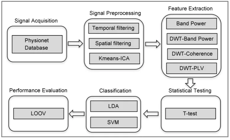
Figure 1. Framework of the proposed BCI system. Signal preprocessing and

feature extraction are performed prior to statistical testing. Selected features are adopted for classification using a LDA and SVM based on a LOOV scheme. ICA: Independent Component Analysis; DWT: Discrete Wavelet Transorm; PLV: Phase Locking Value; T-test: Student test; LDA: Linear Dis-criminant Analysis; SVM: Support Vector Machine; LOOV: Leave One Out Corss Validation.

from signal acquisition until classification. Interestingly, two challenges faced in the BCI research are conducted here: the first consists of adequate preprocessing of EEG signals especially those contaminated with ocular artifacts. The second tackles the identification of the right-hand motor imagery state. There-fore, we will start by presenting the pre-processing techniques while focusing on the proposed Kmeans-ICA ocular artifact rejection method. Then feature extraction, classification and performance evaluation methods are presented and discussed.

2.1. Signal Acquisition

An international database, “PhysioNet.org”, is used in this study. It contains several datasets covering different physiological effects. The “EEG Motor Movement/Imagery dataset” is selected. This database was recorded using the international BCI2000 instrumentation system [13]. It contains 64 channels scalp EEG recordings sampled at 160 Hz. The total database includes 109 subjects who performed 14 motor imagery trials. Electrodes were positioned as per the 10-10 international system, a standard of the American clinical neurophysiology society and the international federation of clinical neurophysiology [14]. In this work, the right-hand motor imagery and relax signals recorded while eyes open are adopted. For more details about the data acquisition experiment, readers are referred to [13].

2.2. Signal Preprocessing 2.2.1. Filtering

(4)

yield a linear phase response. Moreover, to remove this linear phase response and achieve a zero-phase filtering, the forward backward technique was adopted by applying the FIR filter to the signal, inverting it in time, reapply the FIR filter and invert the signal back. In addition, a spatial filtering was used to increase the Signal to Noise Ratio (SNR) what may lead to a better classification of the motor imagery states. Dif-ferent types of spatial filtering were proposed in the literature but several studies have shown that Com-mon Average Reference (CAR) is the best suited for BCI applications [15]. The spatial filter should be de-signed in a way to maximally accentuate the control signal while attenuating non-EEG artifacts. This can be achieved by subtracting the common electrical brain activity to a defined point of interest (1).

1 ˆ

i

i i i j

V V V

N ∈ω

= −

∑

₍₁₎

where Vi and Vˆi are electrode potentials respectively prior and after filtering respectively, and ωi is a

group of the N surrounding channels.

2.2.2. Ocular Artifacts Rejection

Our group has recently proposed a non-supervised ocular artifact rejection method combining ICA and Kmeans clustering [7]. In this work, we validate the proposed methodology and use it within the con-text of a motor imagery classification enforced by statistical assessment and adequate performance evalua-tion. Due to the overlapping nature of ocular artifacts, advanced signal processing techniques based on BSS have been introduced [16]. A BSS method is based on having N unknown sources S, an unknown op-erator A, and N observed signals X (2).

X =AS (2)

ICA was proposed within the framework of BSS techniques. The main idea consists of finding the weights matrix A that will separate the original multichannel signal into non-Gaussian, statistically inde-pendent components. While several ICA algorithms exist, the Extended-Infomax algorithm has been used in this work. It had been previously demonstrated that Extended-Infomax outperformed other ICA algo-rithms, especially for signals containing sup and sub-Gaussian components simultaneously [16]. Some ICs are typically ocular related electrical activity (artifacts) and should be removed. This is traditionally done manually by studying activations’ frequency content and scalp topographies [11]. Our main concern is to automatically find artefactual ICs and omit them from the signal’s reconstructed part.

2.2.3. Automatic Artifact Identification—Feature Extraction

To automate the process of Ocular Artifact identification, three features were adopted and introduced into a Kmeans clustering algorithm [7]. The first feature consists of computing the average of cross corre-lation between each IC with pre-frontal electrodes (FP1 and FP2) as shown in (3). Our motivation behind using this feature is that frontal electrodes are the most contaminated by EOG noise [4].

( )

(

fp ,IC i₁ _{( )} fp2,IC i_{( )}

)

Avrg i = R +R 2 (3)

The cross correlation is implemented as a measure of similarity between two-time series. Rab is the cross correlation between the two signals a and b (4). The closer the absolute value is to 1 the more the signals are correlated.

[ ] [

]

ab n

R =

∑

+∞_=−∞a n ∗b n+k (4)

where k is the time delay between a and b.

The second feature is the distribution ratio; it consists of dividing the maximum amplitude of an IC by its standard deviation (5). Adopting such a characteristic is based on the fact that non-artefactual EEG activity is tightly distributed around its mean [4].

( )

(

)

( )

(

)

Ratio 2

max

Dist IC i

IC i

δ

(5)

The third one is the maximum value of each IC. Our assumption behind proposing it relies on the fact that ocular artifacts are higher in amplitude than normal neurological signals and their peak are commonly centered [5]. This resulted in three feature vectors that will be used as inputs to a Kmeans clus-tering algorithm to identify artefactual ICs.

2.2.4. Kmeans Clustering—Classifying ICs

A Kmeans clustering algorithm was used in this study to classify ICs into artefactual and physiologi-cal components [7]. The Kmeans clustering algorithm performs an iterative minimization of the sum of squared distances from all elements in a cluster to the cluster center [17]. The mathematical principle of this algorithm, applied to our framework is briefly explained. Let’s consider a set of ICs (6).

( ) ( ) ( )

( )

{

}

ICs IC 1 , IC 2 , IC 3 ,, IC l (6)

The algorithm starts by dividing this set into 2 clusters (7) (8):

( )

1

IC1 1 , IC1 2 , IC1 3 ,, IC1 l (7)

( )

2

IC2 1 , IC2 2 , IC2 3 ,, IC2 l (8)

Then the local means of each group are computed and the new grouping is defined as (9) (10)

( )

1

IC1 k −C1< IC1 k −C2 fork =1,, ;l (9)

( )

2

IC2 k −C2 < IC2 k −C1 fork=1,, ;l (10)

where Ci is the center of cluster i.

In such a way, ICs in cluster 1 are closer to C1 and ICs in cluster 2 are closer to C2.

2.2.5. Evaluation of the Proposed Method

Since the proposed approach consists of a classification of the ICs, we started by assessing the accura-cy of the proposed method in identifying artefactual components. Traditional performance descriptors were used: accuracy, sensitivity, specificity, and precision. A true detection of an eye blinking artifact is considered as a true positive event. Accuracy refers to the percentage of correct predictions. Specificity determines the percentage of correctly negative labeled samples classified as negative, while sensitivity in-dicates the percentage of positive labeled samples classified as positive and precision refers to the positive predictions that are correctly classified. Therefore, the sensitivity of the test represents its ability to detect the presence of the event, in this part of the paper, the eye blinking artifact, while the specificity quantifies its performance in identifying the absence of the eye blinking artifact. Performance descriptors were com-puted over 640 samples (a total of 6,400,000 data points).

2.3. Motor Imagery Based BCI: Feature Extraction

After signal preprocessing, a right-hand motor imagery based BCI was implemented. It starts by ex-tracting features able to show relevant information about different brain states. Each of these features is passed through a statistical test to verify it represents a statistically significant difference between motor imagery and relax states. Four features were used in this work. First, the band power of the mu rhythm, a state of art feature in motor imagery classification was computed and used as an input to the classifier. The three remaining features combine the Discrete Wavelet Transform (DWT) with respectively the Band Power, the PLV, and the coherence. These features were chosen since they provide information about properties (power and frequency cross correlation) and dynamics (phase locking value) of brain mental states and thus will contribute to the design of an interpretable BCI.

2.3.1. Band Power Feature

(6)

the event related desynchronization in the contralateral brain region (11).

( )

2

( )

t

X t = x t (11)

Motor imagery (planning of a movement) and movement are respectively characterized by the currence of Event Related Desynchronization (ERD) and Event Related Synchronization (ERS). ERD oc-curs contralaterally in the mu and beta rhythms, while ERS ococ-curs in the beta rhythm, at the ipsilateral side [4]. The Power Spectral Density (PSD) shows a decrease during an ERD and an increase during an ERS [18].

2.3.2. Discrete Wavelet Transform

The wavelet transform is a multi-resolution decomposition allowing signal analysis at multiple scales and resolutions simultaneously so that low frequencies could be examined with high frequency resolution and high frequencies could be studied considering a high temporal resolution (12).

( )

,

( )

,

( )

d

x u s

W s u +∞X t t t

−∞

=

_∫

∅ (12) Each wavelet is a translated and scaled version of the mother wavelet (13).

( )

,

1

a b

t b t

a a

−

 

∅ = _∅ _

  (13)

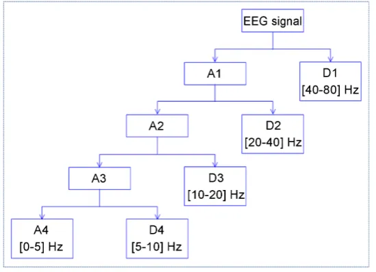
In this study, the DWT was implemented in a discrete way in terms of a series of discrete low- and high-pass filters, decomposing the signal into approximations and details. This decomposition is well de-scribed by the Mallat algorithm as shown in Figure 2.

Equation (14) depicts the frequency bounds of detail levels obtained by wavelet transforming an EEG signal sampled at Fs.

1 1 2

0, , , , , ,

2

2 2 2 2

s s s s s

L L L

F F F F F

+ +

     

     

       (14)

[image:6.595.162.437.475.674.2]

The EEG signal has been decomposed by DWT using Debauchies 5 mother wavelet due to its extreme phase and high number of vanishing moments [19]. Since the Physionet database was recorded and sampled

Figure 2. Wavelet decomposition of the EEG signal. A1,

A2, A3, A4 are approximation levels of the signal while

(7)

at 160 Hz, a four levels’ wavelet transform was performed to depict the Mu rhythm. Three features have been extracted from the D4 mu rhythm level. These features are the DWT-Band Power, DWT-PLV, and DWT-Coherence.

2.3.3. DWT-Coherence

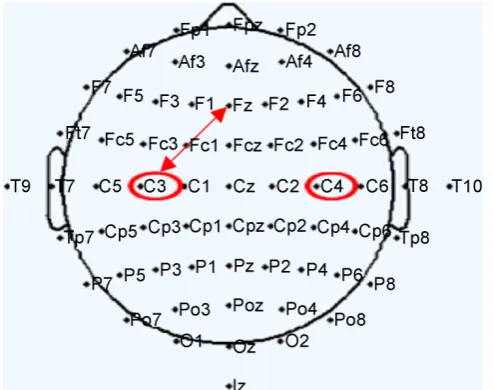
The DWT-Coherence feature starts by a DWT decomposition and then calculate the coherence be-tween electrodes C3 and C4 during right hand motor imagery and relax states (15). Physiologically, due to the occurrence of an event related desynchronization (ERD) on electrode C3 but not on C4 (contralateral electrode) during the right-hand motor task, the coherence is expected to decrease.

2 1

2 2

1 1

* *

0.5 b

b

xy _b _b

b b

x y x y C

x x y y

+ =

⋅

∑

(15)

[image:7.595.177.424.448.643.2]

where x and y are the Fourier transformed temporal signals and b1, b2 the frequency limits of interest. Figure 3 shows 2D representation of the locations of the electrodes involved in computing this feature.

2.3.4. DWT-Phase Locking Value

The phase locking value is used to quantify coupling and phase synchrony between time series. It has been introduced as a feature for BCI applications [20]. Considering two signals x(t) and y(t) and their cor-responding phase’s ∅x

( )

t and ∅y

( )

t , their phases’ difference usually fluctuates around a constant

val-ue as shown in (16).

( )

constant value

x t y t

∅ − ∅ = ₍₁₆₎

Two steps are performed to estimate the phase synchrony; the first consists of estimating the instan-taneous phase of each EEG signal. This is usually computed by means of the analytic signal using the Hil-bert Transform. For each signal x(t), the analytic signal z(t) is a complex function defined as follows (17):

( )

ˆ

( )

z t =x t + jx t (17)

Figure 3. Position of the electrodes involved in

(8)

( )

1

( )

ˆ d π s x t t τ τ τ ∞ −∞ = −

∫

(18) where x tˆ

( )

is the Hilbert transform of x(t). The phase of the signal x(t) is deduced as in (19):

( )

t arctan x tˆ

( )

_{( )}

x t

 

∅ = _ _

  (19)

The second step is to evaluate the amount of phase locking by integrating the phase difference over time for each trial (20).

( )

PLV= ej∆∅t (20)

If the signals are completely synchronized, ∆∅

( )

t is a constant resulting in PLV = 1; otherwise,

( )

t

∆∅ _{follows a uniform distribution and the PLV tends to zero. Local and large scale synchrony are the}

most implemented in the literature of brain human history [21]. Local scale is computed between neigh-boring electrodes while large-scale involves relatively distant electrodes.

In this paper, large scale phase locking was investigated between electrodes Fz and C3. The ERD on electrode C3 may trigger a decrease in synchrony between C3 and Fz; the latter one not influenced by the ERD. Figure 3 shows a 2D mapping of the electrodes involved in computing the DWT-PLV features.

2.4. Statistical Test

A statistical t-test was used to verify which features are significantly different between relax and mo-tor imagery states. The features for which a statistically significant difference is found between relax and motor imagery states will be used as inputs to the classifier. The t-test may be used under normality as-sumption and has been commonly used in BCI studies [22]. It has shown to be one of the most conserva-tive tests used for detecting significant differences using a statistic based on the means of the two sets (21).

1 2 2 2 1 2 1 2 x x T s s n n − = + (21)

A significance level of 0.05 is used in this study.

2.5. Classification

After quantitative features have been extracted, each signal might be represented by a feature vector and used as input to the classifier. In this study, a SVM and a LDA are compared.

2.5.1. Linear Discriminant Analysis

LDA is one of the most effective linear classification methods successfully implemented in BCI appli-cations [23]. A LDA classifier is mainly based on a statistical procedure that defines a criterion function

J(w) that should be maximized. This function requires projecting the n-dimensional data into a line

T

y=w x.

The first step is to compute the sample and projected mean in each class as shown respectively in (22) and (23):

1 Sample

i

i x X

i

m x

k ∈

  =  

 

∑

(22)

T T

1 1

Proj.

i i

i y Y x X i

i i

m y w x w m

k ∈ k ∈

   

= −_{ } =_{ } =

(9)

where ki is the number of samples in class i and Xi is the set of vectors in the class i. A 2-class problem will be expressed as in (24):

(

)

T

1 2 1 2

m −m =w m −m (24)

Considering a class i, the scatter for projected samples is defined as:

(

)

2

i

i y Y i

s =

∑

_∈ y−m (25)

The Linear discriminant, known as the Fisher Discriminant is the function wT_x_{for which}_J₍_w_{) is at its}

highest possible values (26).

( )

₍

1 2

₎

2

2 2 1 2 m m J w s s − =

+ (26)

However, in this expression, J is not as function of w. Let’s define the scatter matrices Si as shown in (27):

(

)(

)

T

i

i x X i i

S =

∑

_∈ x−m x−m (27)

The within class scatter Sw and the between class scatter SB will be computed as shown respectively in (28) and (29).

1 2

w

S =S +S (28)

(

)(

)

T

1 2 1 2

B

S = m −m m −m (29)

Thus, si is defined as in (30)

(

_T _T

)

2 _T

i

i x X i i

s =

∑

_∈ w x−w m =w S w (30)

Therefore, the criterion J(w) is expressed a in (31)

( )

T_T B

w

w S w J w

w S w

= (31)

Using a non-parametric classifier (like LDA) gives a stable basis of comparison between several fea-tures and avoids any interference such as those provoked from the SVM training.

2.5.2. Support Vector Machine

Support Vector Machine (SVM) is one of the most recently adopted classifiers able to create non-linear decision boundaries [20]. It is mainly a binary classifier but it can be extrapolated to solve mul-ti-class problems. Given a set of features with associated labels

{

yi:yi∈ −

{ }

1,1

}

then the training

algo-rithm attempts to find a hyper plane allowing a maximum separation between support vectors corres-ponding to y_i =1 and y_i = −1.

The simplest hyper plane is the linear one, for example, separating two classes (32):

(

w x⋅

)

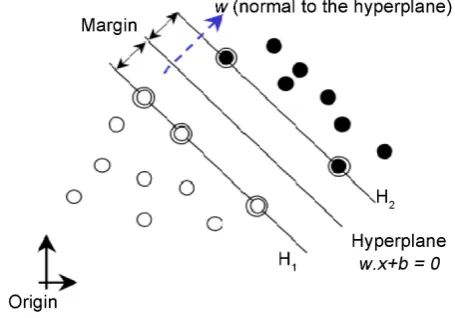
+ =b 0 (32)

The optimal hyper plane is the one that maximizes the distance between the nearest training points.

Figure 4 shows the classification hyper plane of a linear SVM.

The minimum distance between H1 and H2 corresponds to 2 w.

Therefore, the optimization problem could be resumed as follow: Minimize w2 subject to

con-straints:

(

)

1 0

i i

y w x⋅ +b − ≥ (33)

(10)

[image:10.595.183.411.74.233.2]

Figure 4.Linear kernel support vector machine.

non-linear separation.

Several kernels have been proposed such as polynomial (34), Radial Basis Function (RBF) (35) and Multi-Layer Perceptron (MLP) (36).

( ) (

, 1

)

p

K x y = x y⋅ + (34)

( )

, exp ₂ 2

2

x y

K x y

σ

_{− −} 

 

=

 

  (35)

( )

, tanh

(

1 2

)

K x y = p x y⋅ + p (36)

The SVM classifier has given good results in BCI research activities [24], however they have several hyper parameters that should be fixed such as the regularization parameter as well as the RBF width when using a non-linear SVM and they show a relatively low speed of execution what would be a constraint in an online BCI system.

3. RESULTS AND DISCUSSION

Results can be divided into two main parts: the first describes the performance of the ocular artifact rejection method; a case is considered for visualization purposes and quantitative evaluation methods are presented. The second covers motor imagery classification performance evaluation.

3.1. Ocular Artifacts Rejection Method

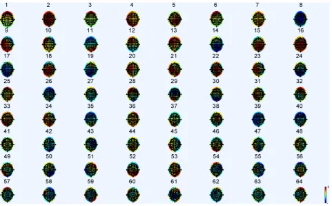
The ocular artifact rejection method was done using Kmeans-ICA. ICA of the 64 channels input sig-nals was performed using the Infomax algorithm. Figure 5 shows scalp topographies of the 64 ICs. By means of visual inspection, in the considered dataset, components 1, 3, and 6 are considered as eye blink-ing artifacts since their scalp maps show an intense frontal projection, typical of an ocular artifact. As al-ready mentioned, an automatic method has been implemented in this paper for detecting these artefactual components and omitting them from the reconstructed signals.

Thus, the correlation, distribution ratio and maximum value features have been considered. Experi-mental results show that components 1, 3, and 6 have the highest value for each of the proposed features.

As mentioned above, IC1, IC3 and IC6 are assumed as ocular artifacts. Figure 6 shows their scalp map projections, typical of an eye artifact. Artefactual components are also identified by a field expert based on ICs’ scalp maps, power spectrum and time series. This serves as our ground truth for perfor-mance evaluation. Accuracy, precision, sensitivity, and specificity were calculated for all feature vectors.

(11)

[image:11.595.59.541.71.369.2]

[image:11.595.127.472.402.502.2]

Figure 5.Scalp topographies of the independent components.

Figure 6. Frontal projection typical of an ocular artifact in 2D

map-ping of IC1, IC2, and IC3.

Table 1.Values of TPs, TNs, FPs, and FNs for all features.

Feature Performance Measure TP TN FP FN Total Correlation 25 612 3 0 640 Distribution Ratio 18 516 12 104 640 Maximum Value 14 618 8 0 640 TP: True positive; TN: True negative; FP: False positive; FN: False negative.

[image:11.595.129.469.576.666.2]

(12)

Table 2 shows the performance of the ocular artifact non-supervised classifier in terms of accuracy, sensi-tivity, specificity, and precision based on 640 samples from all subjects. Three features were used for classi-fication; when used independently, the correlation feature gives the highest accuracy (99.54%) and will be considered for the identification of artefactual ICs in the next parts of this paper.

Prominent results were also obtained for other features especially for the maximum value, an easy to compute, simple feature. These prominent results highlight the feasibility of automatic ocular artifacts re-moval from EEG signals based on ICA.

3.2. Motor Imagery Classification

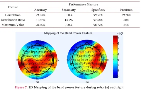
3.2.1. Mapping of the Band Power Feature

The four physiologically interpretable features adopted were the Band power, DWT-Band power, DWT-PLV and DWT-Coherence. A 2D mapping of the band power feature over the sensorimotor area is shown during the relax state (Figure 7(a)) and right hand motor imagery state (Figure 7(b)). The mu-rhythm band power shows a contralateral decrease (left) during the right-hand motor imagery state.

3.2.2. Results of the Statistical Test

In order to quantify the discriminative power of these features, significance difference has been tested between relax and motor imagery states using the t-test, a statistical significance test applied to small data sets. Table 3 shows the results of the t-test at a significance level of 0.05. The null hypothesis was rejected for Band Power, DWT-Coherence, and DWT-PLV suggesting that there is a significant difference between the two states (Table 3). Thus, these features will be use as inputs to the classifier.

Table 2. Results of the ROC analysis.

Feature Performance Measure

Accuracy Sensitivity Specificity Precision Correlation 99.54% 100% 99.51% 89.28% Distribution Ratio 81.87% 14.7% 97.68% 60%

[image:12.595.61.543.384.694.2]

Maximum Value 98.75% 100% 98.72% 64%

Figure 7. 2D Mapping of the band power feature during relax (a) and right

(13)

3.2.3. Classification Using a LDA

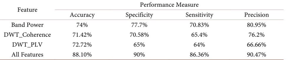
[image:13.595.54.548.339.444.2]

This type of validation is the most used on EEG signals where the amount of data for each subject is li-mited. The population consists of three subjects (50 signals/trials). Table 4 shows the results of the cross validation using a LDA after ocular artifact removal based on Kmeans-ICA. Results show that the best performance is obtained after ocular artifact removal using the three features together (Table 4) achieving a relatively good performance considering non-physiological interferences (e.g. extreme values and base-line drifts) common in the Physionet database. These artifacts would highly affect the recognition rate of the classifier. Additionally, to evaluate the suitability of the “Kmeans-ICA” ocular rejection method in the context of a motor imagery classification, the LOOV based on a LDA was performed on the ocular artifact contaminated EEG signals.

Table 5 illustrates the results of LOOV without ocular artifact removal. Results show that the classifi-cation accuracy based on the three features increased from 66% to 88.10% after removing ocular artifacts by means of “Kmeans-ICA”.

3.2.4. Classification Using a SVM

Classification based on a support vector machine was also implemented. LOOV was performed on the same signals after Kmeans-ICA filtering while using different kernel functions. A sequential minimal

Table 3. Results of the statistical test.

Statistical Measure

Feature

Band Power DWT-Band Power DWT-Coherence DWT-PLV

H 1 0 1 1

P 6.1795e−07 _0.6434 _0.0068 _4.1535e−04

[image:13.595.57.546.481.584.2]

Result Null Hypothesis _Rejected Null Hypothesis _Conserved Null Hypothesis _Rejected Null Hypothesis _Rejected

Table 4. Results of the LOOV after Kmeans-ICA using a LDA.

Accuracy Specificity Sensitivity Precision Band Power 74% 77.7% 70.83% 80.95% DWT_Coherence 71.42% 70.58% 65.4% 76.2%

[image:13.595.56.547.620.727.2]

DWT_PLV 72.72% 65% 64% 66.66% All Features 88.10% 90% 86.36% 90.47%

Table 5. Results of the LOOV without ocular artifact removal.

Accuracy Specificity Sensitivity Precision Band Power 66.66% 70.58% 64% 76.19% DWT_Coherence 57.14% 58.82% 59.25% 66.6%

(14)

optimization algorithm was used to find the separating hyper plane using the following kernel functions: linear, polynomial, RBF and MLP. The highest accuracy was obtained using a linear kernel function based on a combination of all features (85.71%); however, using an LDA classifier gave a better accuracy (88.10%). RBF, Polynomial, and MLP kernel gave accuracies of 80.95%, 76.20%, and 73.80% respectively using the combination of all features. As mentioned, an LDA is easier to implement, simpler and less time consuming what make it suitable for online BCI applications. Worth to mention, the accuracies were ob-tained from signals recorded across many sessions and many subjects and are therefore subject to in-ter-session and inter-subject variability. Usually, in a BCI system, there is a phase of calibration, in which the classifier is well adapted to each subject. This phase will probably increase the accuracy since each sys-tem will be adapted to its user’s brain states and this is an ongoing research.

Using a combination of three interpretable features as inputs to the LDA classifier, the BCI system reached a classification accuracy of 88.10% while differentiating between relax and right hand motor im-agery states. Considering the Physionet signal population and for comparison, a classical BCI system based solely on the traditional, most widely used band power feature gave an accuracy of 74% what highlights the performance of the proposed system.

4. CONCLUSIONS

A BCI-based system was proposed for the right-hand motor imagery classification. It uses an auto-matic ocular artifact rejection technique that does not require adding an EOG reference channel. Its prin-ciple mainly relies on ICA to which simple and easy to implement features were added to automate the algorithm. Ocular artifacts are identified by means of a non-supervised machine learning technique: Kmeans clustering. Results show that the proposed method is effective in terms of ocular artifact identifi-cation, removal and conservation of neurological signals. This is supported by the increased accuracy of the motor imagery classification after Kmeans-ICA.

Additional preprocessing techniques were also used such as temporal and spatial filtering in order to remove other types of artifacts. Three physiologically interpretable features: band power, DWT-PLV and DWT-Coherence were used for the classification. Results show that the use of Kmeans-ICA has increased the accuracy of the classification that reached 88.10% when using a linear discriminant analysis classifier considering the inter-subject and even inter-session variability (compared to 66% without Kmeans-ICA filtering). This is due to the fact that ocular artifact removal increases the discriminant stability of the EEG data when eliminating the high influence of the EOG noise and maintaining the EEG of interest what will increase the recognition rate of the BCI system.

Two classifiers were compared: 1) a LDA and 2) a SVM with regards to BCI applications. The use of the Kmeans-ICA method could be extended to more applications other than BCI ones such as general EEG denoising. ICA is being more extensively used as a preprocessing tool in software that provides solu-tions for neurophysiological research; however current solusolu-tions are limited to a manual classification of the ICs. The implementation of a module based on the proposed method would be helpful and reduce the variability due to different interpretation of scalp topographies.

ACKNOWLEDGEMENTS

The authors acknowledge financial support form he Canada Research Chair in Smart Medical Devices and the Higher Research Center (CSR) – USEK.

REFERENCES

1. Vidal, J.J. (1973) Toward Direct Brain-Computer Communication. Annual Review of Biophysics and Bioengi-neering, 2, 157-180.https://doi.org/10.1146/annurev.bb.02.060173.001105

(15)

Medi-https://doi.org/10.4236/jbise.2017.106025 340 J. Biomedical Science and Engineering

cine, 3, 1-8.https://doi.org/10.1109/JTEHM.2015.2485261

3. Delgado Saa, J.F. and Cetin, M. (2013) Discriminative Methods for Classification of Asynchronous Imaginary Motor Tasks from EEG Data. IEEE Transactions on Neural Systems and Rehabilitation Engineering, 21, 716- 724.https://doi.org/10.1109/TNSRE.2013.2268194

4. Sanei, S. and Chambers, J.A. (2007) EEG Signal Processing. John Wiley & Sons Ltd., 35-125. https://doi.org/10.1002/9780470511923

5. Assi, E.B. and Rihana, S. (2014) Kmeans-ICA Based Automatic Method for EOG Denoising in Multi-Channel EEG Recordings. Proceedings of 11th IASTED International Conference on Biomedical Engineering, Zurich, 23-25 June 2014, 233-238.

6. Kroupi, E., Yazdani, A., Vesin, J.M. and Ebrahimi, T. (2011) Ocular Artifact Removal from EEG: A Comparison of Subspace Projection and Adaptive Filtering Methods. 19th European Signal Processing Conference, Barcelo-na, 2011, 1395-1399.

7. Assi, E.B., Rihana, S. and Sawan, M. (2014) Kmeans-ICA Based Automatic Method for Ocular Artifacts Remov-al in a Motorimagery Classification. Engineering in Medicine and Biology Society (EMBC), 2014 36th Annual International Conference of the IEEE, Chicago, IL, USA, 26-30 August 2014, 6655-6658.

https://doi.org/10.1109/EMBC.2014.6945154

8. Croft, R.J. and Barry, R.J. (2000) Removal of Ocular Artifact from the EEG: A Review. Clinical Neurophysiolo-gy, 30, 5-19. https://doi.org/10.1016/S0987-7053(00)00055-1

9. Gotman J., Skuce, D.R., Thompson, C.J., Gloor, P., Ives, J.R. and Ray, W.F. (1973) Clinical Applications of Spectral Analysis and Extraction of Features from Electroencephalograms with Slow Waves in Adult Patients.

Electroencephalography and Clinical Neurophysiology, 35, 225-235.

10. Lagerlund, T.D., Sharbrough F.W and Busacker, N.E. (1997) Spatial Filtering of Multichannel Electroencepha-lographic Recordings through Principal Component Analysis by Singular Value Decomposition. Journal of Clinical Neurophysiology, 14, 73-82.https://doi.org/10.1097/00004691-199701000-00007

11. Romero, S., Mananas, M.A., Riba, J., Morte, A., Gimenez, S., Clos, S. and Barbanoj, M.J. (2004) Evaluation of an Automatic Ocular Filtering Method for Awake Spontaneous EEG Signals Based on Independent Component Analysis. 26th Annual International Conference of the IEEE Engineering in Medicine and Biology Society,San Francisco, CA, 1-5 September 2004, 925-928. https://doi.org/10.1109/iembs.2004.1403311

12. Joyce, C.A., Gorodnitsky, M., I.F. and Kutas, M. (2004) Automatic Removal of Eye Movement and Blink Arti-facts from EEG Data Using Blind Component Separation. Psychophysiology, 41, 313-325.

https://doi.org/10.1111/j.1469-8986.2003.00141.x

13. Goldberger, A.L., Amaral, L.A.N., Glass, L., Hausdorff, J.M., Ivanov, P.C., Mark, R.G., et al. (2000) PhysioBank, PhysioToolkit, and PhysioNet: Components of a New Research Resource for Complex Physiologic Signals. Cir-culation, 101, e215-e220. https://doi.org/10.1161/01.cir.101.23.e215

14. Nuwer, M.R. (1987) Recording Electrode Site Nomenclature. Journal of Clinical Neurophysiology, 4, 121-133. https://doi.org/10.1097/00004691-198704000-00002

15. McFarland, D.J., McCane, L.M., David, S.V. and Wolpaw, J.R. (1997) Spatial Filter Selection for EEG-Based Communication. Electroencephalography and Clinical Neurophysiology, 103, 386-394.

16. Brunner, C., Delorme, A. and Makeig, S. (2013) Eeglab—An Open Source Matlab Toolbox for Electrophysio-logical Research. Biomedizinische Technik, 58. https://doi.org/10.1515/bmt-2013-4182

17. Reddy, N.P. (2002) Biomedical Signal Analysis: A Case-Study Approach, by Rangaraja M. Rangayyan. Annals of Biomedical Engineering, 30, 983-983. https://doi.org/10.1114/1.1509766

(16)

https://doi.org/10.4236/jbise.2017.106025 341 J. Biomedical Science and Engineering Computer Interface. 2013 2nd International Conference on Advances in Biomedical Engineering,Tripoli, 11-13 September 2013, 30-33. https://doi.org/10.1109/icabme.2013.6648839

19. Hsu, W.Y. (2012) Application of Competitive Hopfield Neural Network to Brain-Computer Interface Systems.

International Journal of Neural Systems, 22, 51-62. https://doi.org/10.1142/S0129065712002979

20. Wang, Y., Hong, B., Gao, X. and Gao, S. (2006) Phase Synchrony Measurement in Motor Cortex for Classifying Single-Trial EEG during Motor Imagery. 28th Annual International Conference of the IEEE Engineering in Medicine and Biology Society, New York, 30 August-3 September 2006, 75-78.

https://doi.org/10.1109/iembs.2006.259673

21. Varela, F., Lachaux, J.-P., Rodriguez, E. and Martinerie, J. (2001) The Brainweb: Phase Synchronization and Large-Scale Integration. Nature Reviews Neuroscience, 2, 229-239. https://doi.org/10.1038/35067550

22. Rice, J. (2001) Mathematical Statistics and Data Analysis. Duxbury Press,Grove, CA.

23. Cohen, M.E. and Hudson, D.L. (1999) Neural Networks and Artificial Intelligence for Biomedical Engineering. Wiley-IEEE Press.

24. Rakotomamonjy, A. and Guigue, V. (2008) BCI Competition III: Dataset II—Ensemble of SVMs for BCI P300 Speller. IEEE Transactions on Biomedical Engineering, 55, 1147-1154.

https://doi.org/10.1109/TBME.2008.915728

Submit or recommend next manuscript to SCIRP and we will provide best service for you: Accepting pre-submission inquiries through Email, Facebook, LinkedIn, Twitter, etc.

A wide selection of journals (inclusive of 9 subjects, more than 200 journals) Providing 24-hour high-quality service

User-friendly online submission system Fair and swift peer-review system

Efficient typesetting and proofreading procedure

Display of the result of downloads and visits, as well as the number of cited articles Maximum dissemination of your research work